

Introduction
The Digital Soil Map of Sweden (DSMS) is a recently developed spatial database of topsoil texture covering >90% of Sweden´s arable land (about 2.4 million ha) (Söderström and Piikki, Reference Söderström and Piikki2016). The data is stored in raster format and has a spatial resolution of 50 m×50 m. It is publicly available under CC-BY license. The DSMS was derived according to the principles for digital soil mapping (McBratney et al., Reference McBratney, Santos and Minasny2003): a prediction model (in this case a Multivariate Adaptive Regression Splines models) was calibrated by soil samples and used for exhaustive predictions of soil properties based on a number of ancillary variables in raster data format (in the case of DSMS: airborne gamma radiation data, airborne laser-scanned digital elevation data, and legacy Quaternary soil maps). The mean absolute error (MAE; Equation 1) of the clay content in DSMS was 5.6% clay but the map accuracy varied between areas, e.g. depending on the geology. The map can be used as decision support for e.g. variable-rate liming for improving soil structure and for variable-rate seeding.
 $$MAE\,{\equals}\,{1 \over n} \mathop{\sum}\limits_{i\,{\equals}\,1}^n {\left| {l_{i} {\minus}m_{i} } \right|} $$
where l i =lab. value for sample i; m i =map value for sample i; n=number of samples.
In order to take advantage of farmers’ own soil texture data, Söderström et al. (Reference Söderström, Sohlenius, Rodhe and Piikki2016a) evaluated a method to use such soil samples to improve the clay content data in DSMS, locally on a farm. They demonstrated that it was possible to reduce the prediction error in more than two-thirds of the farms by including the local soil samples in the calibration dataset and giving them extra weight (according to the principles sometimes applied in spiking in spectroscopic analyses; Wetterlind and Stenberg, Reference Wetterlind and Stenberg2010). Applying a method for local adaptation (in effect downscaling) of a digital soil database may be preferred, in some cases, compared to recalibrating the soil database. It is not necessary for the user to have access to all predictor and calibration datasets, and the local adaptation, can be performed directly without need for data harmonization procedures. This was for example shown by Söderström et al. (Reference Söderström, Piikki and Cordingley2016b) in a study in Rwanda where the global soil database SoilGrids (Hengl et al., Reference Hengl, de Jesus, Heuvelink, Gonzalez and Kilibarda2016) were downscaled and improved using local soil analyses. The aim of the present study was to test two different adaptation methods (residual kriging and regression kriging) that can be applied to a regional digital soil map without access to the geodata used to derive it. Specifically, the aim was:
-
1. To compare farmwise mean absolute errors (MAEs) for an original map (DSMS), the two different adaptation methods, and independent use of soil samples for derivation of farm maps (inverse distance weighting).
-
2. To summarize MAEs of the different methods in relation to variation range of the farms.
-
3. To test the statistical significance of any improvement achieved by using the locally best map compared to consistently using any of the four methods described above.
Materials and methods
Validation data
A data set of clay content analysed in 12,528 topsoil samples was obtained for the present project by the Swedish Board of Agriculture. As there was no farm identity available (i.e. it was not which fields were managed by the same farmer), the dataset was spatially clustered into 403 artificial farms (any farm had at least five clay samples). The sampling density was one clay analysis per three ha. This validation dataset had approximately the same extent as the DSMS (i.e. the southern third of Sweden).
Validated methods
Four different methods were compared. These were:
-
∙ Map only: Using DSMS as it is, without local adaptation. This is currently the default map available to farmers.
-
∙ Adapted map 1: The DSMS was adjusted by residual kriging. Data was extracted from DSMS at the soil sample locations. The residuals (difference between laboratory analysis of clay content and DSMS map value) was calculated and interpolated by ordinary kriging, using an automated procedure with a standard variogram model circumventing the general principles of the number of observations generally required in geostatistics (spherical model with range=400 m, nugget=10% of the variance of the residuals and partial sill=90% of the variance of the residuals). The adapted clay content was then calculated as the sum of the interpolated residuals and the DSMS value.
-
∙ Adapted map 2: The DSMS was adjusted by regression kriging; a linear regression model between the laboratory values and the DSMS values was parameterized. Predictions were made for each sample location and the residuals (difference between laboratory analysis and the value predicted by the regression model) was calculated. These residuals were kriged (automated variogram as described above) and added to the regressed value to yield the adapted clay content value.
-
∙ Samples only: The laboratory analysed clay content values of the soil samples were interpolated by inverse distance weighting (IDW; power=2). This is common practice in most Swedish soil laboratories when a farmer has carried out soil sampling.
Validation strategy
Validation was carried out farm by farm. Data from DSMS were extracted for the sample locations. The adapted map methods (residual kriging and regression kriging) and the samples only method (IDW) were cross-validated by leaving one sample out at a time. MAE values were calculated for each farm and the method with the lowest MAE was considered the best method.
Statistical tests and software
A statistical analysis was undertaken to compare the performance of the best method with the other four methods based on reduction in MAE. Paired t-tests with the null hypothesis (H 0 ) that there was no difference in average MAE were carried out between each of the four methods and the best method strategy. The replicates were the 403 farms. Spatial data management was carried out using ArcGIS (ESRI, Redlands, CA, USA). Data analyses were carried out in R (R Core Team, Reference R Core2016), packages rgdal, Sp, raster, gstat, maptools and rgeos. Statistical tests and plotting of results were made in Excel (Microsoft, Redmond, WA, USA).
Results
Descriptive statistics
Descriptive statistics for the number of samples per farm and the clay content range per farm are found in Table 1. The dataset consisted of a wide range of farm sizes and clay content variabilities.
Table 1 Descriptive statistics of farmwise measures summarized for the 403 farms. Q1 and Q3 are quartiles of the frequency distribution.
Cross-validation results
The best method varied for each farm (Fig. 1). The results were summarized for different clay content ranges within the farms and there is a notable trend that the Adapted map 1 method (residual kriging) performed better the wider the clay content variation range. The opposite trend was observed for all other methods (Fig. 1). In total, using the Samples only-method was best in 31% percent of the cases, while DSMS performed best in 15% of the farms. Adapted map 1 (residual kriging) yielded the lowest MAE in 35% of the farms whereas Adapted map 2 was the best method to use in 19% of the farms.
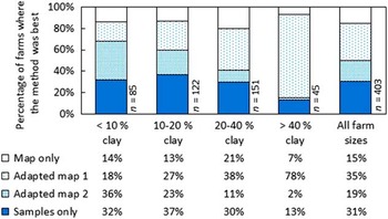
Figure 1 Percentage of farms where each method performed best (had the lowest mean absolute error, MAE) in relation to the clay content variation range of the farms.
Validation of the Best method-strategy
Running an R script that tests all methods and selects the one with lowest MAE (‘the best method strategy’) meant a statistically significant reduction in MAE, compared to consistent use of any of the other methods (p<0 .001 in all four cases; Figure 2). The overall MAE in the present study was 4.6% clay and the overall MAE, when using the best method at each farm, was 3.2% clay.

Figure 2 Average of farmwise mean absolute error (MAE) for the 403 farms. Error bars denote inter-quartile range. Results from the paired t-tests between the Best method and the consistent use each of the four other methods are presented above the error bars. ***=p<0.001.
Discussion
In one part of Sweden it has previously been demonstrated that a regional digital soil map can be improved locally by adding a number of texture analyses from a farm (Söderström et al., Reference Söderström, Sohlenius, Rodhe and Piikki2016a). This was tested on 56 farms using a total of 1,968 soil samples. The present study of almost national coverage, based on 12,528 soil samples, confirmed that result, albeit using two other adaptation methods. The adapted digital soil map had a lower MAE than both the original digital soil map and the traditionally interpolated maps in 54% of the examined farms.
An interface for local adaptation of DSMS has been developed (in R) in an automated, free web application for Swedish farmers (http://markdata.se) aiming at deriving prescription files for variable seeding rate and variable lime application for improvement of soil structure. Based on the present study, the best method strategy will be implemented in this web service.
Conclusion
In some areas, the regional digital soil map was better than topsoil clay content maps obtained by local sampling and traditional mapping (31% of farms). In other areas the opposite was true (15% of farms) and in the remaining 54% of the 403 validated farms, the best method was to adapt the digital soil map by use of local samples (residual kriging or regression kriging). Choosing the locally best method for each farm, significantly (p<0.001) reduced the MAE of produced soil maps compared to consistent use of any other method. Utilization and local adaption of regional digital soil maps for generating prescription files for within-field use is recommended.
Acknowledgements
The present project was funded by Stiftelsen Lantbruksforskning (Contract: O-15-20-566).


