


Implications
This paper introduces a nonlinear profit-maximizing diet formulation problem for beef cattle based on well-established predictive equations. We develop a mathematical model that can guarantee an exact solution for maximum profit diet formulations. This contrasts with widely used but less robust least-cost diet formulation approaches. Our method can efficiently solve an often-impractical nonlinear problem by solving a finite number of linear problems. By optimizing ration formulation on feedlot systems, this work contributes to the sustainable intensification of livestock production.
Introduction
Cattle system profit margins can be small compared to other land uses (Pashaei Kamali et al., Reference Pashaei Kamali, van der Linden, Meuwissen, Malafaia, Oude Lansink and de Boer2016) and nutrient supply is the largest production cost element, for example, for feedlot finishing systems in Brazil, feeding can represent as much as 88% of variable costs, disregarding animal purchase (Sartorello et al., Reference Sartorello, Bastos and Gameiro2018). Feeding cattle with on-pasture supplementation or feedlot diets intensifies production by increasing animal efficiency and profitability, compared to extensive pasture-based systems (Kaimowitz and Angelsen, Reference Kaimowitz and Angelsen2008). By shortening the animal production cycle and therefore reducing methane (CH4) from ruminant enteric fermentation (Cortez-Arriola et al., Reference Cortez-Arriola, Groot, Rossing, Scholberg, Améndola Massiotti and Tittonell2016), feedlots may also decrease the greenhouse gas emissions intensity per unit product by around 25% compared to extensive systems in Brazil (de Gouvello Filho and Hissa, Reference de Gouvello Filho and Hissa2011). Increasing the adoption of these measures is, therefore, desirable from different sustainability perspectives.
Ration formulation is a complex problem typically analyzed using mathematical optimization (Hertzler et al., Reference Hertzler, Wilson, Loy and Rouse1988; Nicholson et al., Reference Nicholson, Lee, Boisvert, Blake and Urbina1994; Tedeschi et al., Reference Tedeschi, Fox, Chase and Wang2000; Soto and Reinoso, Reference Soto and Reinoso2012; Garcia-Launay et al., Reference Garcia-Launay, Dusart, Espagnol, Laisse-Redoux, Gaudré, Méda and Wilfart2018). Ration formulation requires empirical and mechanistic equations to predict growth and nutrient requirements as functions of animal characteristics and the diet composition (Tedeschi et al., Reference Tedeschi, Fox, Sainz, Barioni, de Medeiros and Boin2005; NASEM, 2016). The nonlinear and dynamic nature of biological responses and lack of data restrict the construction of completely mechanistic models. Thus, animal nutrition models rely on a statistical fit of available data, and a mix of mechanistic and empirical equations to predict physiological functions (Tedeschi et al., Reference Tedeschi, Fox, Sainz, Barioni, de Medeiros and Boin2005). This nonlinear characteristic of biological systems is a complicating factor in diet optimization models.
The objective of this paper is to derive a method to optimize maximum profit diets. We introduce and analyze a nonlinear profit-maximizing diet model based on the latest version of the ‘Nutrient Requirements for Beef Cattle’ by NASEM (2016). However, any cattle growth predictive model that can be parametrically linearized can be solved using this approach. We propose a new methodology to solve a nonlinear profit-maximizing cattle diet efficiently. We further explore how performance may be improved between linear and logarithmic time complexity. This paper is structured in four sections. Firstly, the ‘Material and methods’ section provides background on diet formulation problems, describes the mathematical model for the nonlinear programming (NLP) problem of a profit-maximizing diet and explores how to obtain an exact solution solving a finite amount of linear programming (LP) problems. The ‘Results’ section shows the solutions using the proposed algorithms, sensitivity analysis on key parameters and convergence. We then discuss in more detail the implications of using the model and uncertainties to be considered. Finally, the ‘Conclusion’ section summarizes our outcomes in terms of its applications and identifies future research. Preliminary results of this work were already published in an abstract form (Marques et al., Reference Marques, Silva, Barioni, Hall and Moran2019).
Material and methods
Background to diet formulation problems
Previous work with a nonlinear diet problem based on the nutrient requirements of beef cattle (NRC, 1984) explored the trade-offs between profit and cost when dealing with diet optimization problems (Hertzler et al., Reference Hertzler, Wilson, Loy and Rouse1988). However, recent work on these equations (NASEM, 2016) hindered the viability of solving a nonlinear problem directly. Detailed descriptions of the evolution of nutrition models for cattle, sheep and goats have been published recently (Tedeschi and Fox, Reference Tedeschi and Fox2020; Cannas et al., Reference Cannas, Tedeschi, Atzori and Lunesu2019; Tedeschi, Reference Tedeschi2019). Tedeschi (Reference Tedeschi2019) recently advanced the development of the Cornell Net Carbohydrate and Protein System achieved in the 1990s (Fox et al., Reference Fox, Sniffen, O’Connor, Russell and Van Soest1992; Russell et al., Reference Russell, O’Connor, Fox, Van Soest and Sniffen1992; Sniffen et al., Reference Sniffen, O’Connor, Van Soest, Fox and Russell1992), allowing researchers to apply heuristic approaches with LP models for least-cost diets (Tedeschi et al., Reference Tedeschi, Fox, Chase and Wang2000; Soto and Reinoso, Reference Soto and Reinoso2012).
Deriving a profit-maximizing beef cattle diet implies the need to address nonlinear animal weight gain associated with the simultaneous change in diet energy concentration and the gain composition of the animal. Many cattle ration formulation studies are based on linear cost-minimizing diets (Oishi et al., Reference Oishi, Kumagai and Hirooka2011 and Reference Oishi, Kato, Ogino and Hirooka2013; Moraes et al., Reference Moraes, Wilen, Robinson and Fadel2012 and Reference Moraes, Fadel, Castillo, Casper, Tricarico and Kebreab2015; Cortez-Arriola et al., Reference Cortez-Arriola, Groot, Rossing, Scholberg, Améndola Massiotti and Tittonell2016; Mackenzie et al., Reference Mackenzie, Leinonen, Ferguson and Kyriazakis2016; Garcia-Launay et al., Reference Garcia-Launay, Dusart, Espagnol, Laisse-Redoux, Gaudré, Méda and Wilfart2018). Linear cost-minimizing diet models based on NASEM (2016) assume a fixed daily shrunk weight gain (SWG) rather than a variable to be determined. Since SWG depends on the concentration of net energy for maintenance (CNEm) and net energy for gain (CNEg) in the diet, the least-cost modeling approach works under the assumption that these are fixed parameters. Unlike cost minimization, profit maximization varies with growth rate and the animal selling price. Then, unless we know optimal CNEm and CNEg beforehand, fixing these parameters hinders the possibility of finding profit-maximizing diets.
Cattle growth model
This work is based on the NASEM (2016) model to predict nutrient requirements and growth in beef cattle, which is frequently reviewed and updated to increase accuracy. Their model includes the Cornell Net Carbohydrate and Protein System mechanistic equations (Fox et al., Reference Fox, Sniffen, O’Connor, Russell and Van Soest1992; Russell et al., Reference Russell, O’Connor, Fox, Van Soest and Sniffen1992; Sniffen et al., Reference Sniffen, O’Connor, Van Soest, Fox and Russell1992; O’Connor et al., Reference O’Connor, Sniffen, Fox and Chalupa1993), recommendations on possible fit adjustments and variable parameters for a broad range of biophysical conditions, including hormones, lactation, sex, breed, climate, heat loss, growing and finishing. Their predictive model for nutrient requirements is especially helpful in pinpointing possible shortfalls that compromise growth and metabolic efficiency. The process of defining the diet composition starts with empirical equations to predict approximate energy, protein and DM intake (DMI) requirements. After determining the diet, nutrient utilization is refined using more sophisticated equations.
Based on animal weight, NASEM (2016) estimates the net energy for maintenance (NEm (Mcal/day)) and metabolizable protein for maintenance (MPm (g/day)) requirements as a function of shrunk BW (SBW), sex (SEX), breed (BE), lactation (L) and acclimatization factor (a2) as:
 $${{\rm{NEm}} = {\rm{SB}}{{\rm{W}}^{0.75}}\left( {0.077\;{\rm{BE\;L}}\left\;( {{\rm{a}}2 + 0.05\;{\rm{}}\left( {{\rm{BCS}} - 1} \right){\rm{SEX}} + 0.8} \right)} \right)$$
 $${\rm{MPm}} = {\rm{}}3.8\;{\rm{SB}}{{\rm{W}}^{0.75}}$$
For a given NEm, the DMI (kg/day) required can be predicted by:
 $${\rm{DMI}} = {\rm{SBW}}\;\left( {1.2425{\rm{}} + {\rm{}}1.9218\;{\rm{NEm}} - {\rm{}}0.7259\;{\rm{NE}}{{\rm{m}}^2}} \right)$$
Dry matter intake required for growing/finishing cattle must also hold:
 $${\rm{DMI}} = {\rm{NEm}}/{\rm{CNEm}} + {\rm{NEg}}/{\rm{CNEg}}$$
where CNEm (Mcal/kg) is the concentration of net energy for maintenance, NEg (Mcal/day) is the net energy available for gain and CNEg (Mcal/kg) is the concentration of net energy for gain (Anele et al., Reference Anele, Domby and Galyean2014).
The daily SWG (kg/day) for the given diet is given by:
 $${\rm{SWG}} = {\rm{}}13.91\;{\rm{NE}}{{\rm{g}}^{0.9116}}\;{\rm{SB}}{{\rm{W}}^{ - 0.6837}}$$
Beef cattle profit-maximizing diet
Given animal attributes, for example, SBW, breed, sex and a set J of possible ingredients, we formulate a diet by defining its composition in terms of the proportion of each ingredient x j ∈ [0, 1] and the respective cost c j (US$/kg of DM) ∀ j ∈ J. Cost per kilogram of DM is readily obtained from cost per kilogram as feed (US$/kg AF) divided by the DM ratio of the ingredient (kg of DM/kg AF) (NASEM, 2016). In T days, total profit Z (US$) can be maximized by the NLP model consisting of equations (6) to (13).
 $$\eqalign{{{\rm{Max\!: }}\;Z{\rm{}} = {\rm{}}T \times 13.91 \times {\rm{}}S} \cr\times {\rm{SB}}{{\rm{W}}^{ - 0.6837}}{\left[ {\left( {\mathop \sum \nolimits_{j \in J} {\rm{cne}}{{\rm{g}}_j}{x_j}} \right)\left( {{\rm{DMI}} - {{{\rm{NEm}}} \over {\mathop \sum \nolimits_{j \in J} {\rm{cne}}{{\rm{m}}_j}{x_j}}}} \right)} \right]^{0.9116}} \cr \hskip -60pt- {\rm{}}T \times {\rm{DMI}}\mathop \sum \nolimits_{j \in J} {c_j}{x_j}}$$
 $$\eqalign{{{\rm{s}}{\rm{.t}}{\rm{.}}\!:\sum\nolimits_{j \in J} {{\rm{m}}{{\rm{p}}_j}{x_j}}} \cr \hskip-50pt\geq {\rm{DM}}{{\rm{I}}^{ - 1}}{\rm{}}\;\left\{ {\matrix{ \cr \cr \cr \cr } } \right.{\rm{}}3.8{\rm\;{SB}}{{\rm{W}}^{0.75}} + 3727.88 \cr \hskip-50pt{\rm{}}{\left[ {\left( {\sum\nolimits_{j \in J} {{\rm{cne}}{{\rm{g}}_j}{x_j}} } \right)\left( {{\rm{DMI}} - {{{\rm{NEm}}} \over {\mathop \sum \nolimits_{j \in J} {\rm{cne}}{{\rm{m}}_j}{x_j}}}} \right)} \right]^{0.9116}} \cr \hskip-50pt{\rm{SB}}{{\rm{W}}^{ - 0.6837}} - {\rm{}}29.4\;{\rm{}}\left[ {\left( {\mathop \sum \nolimits_{j \in J} {\rm{cne}}{{\rm{g}}_j}{x_j}} \right)\left( {{\rm{DMI}} - {{{\rm{NEm}}} \over {\mathop \sum \nolimits_{j \in J} {\rm{cne}}{{\rm{m}}_j}{x_j}}}} \right)} \right]\left. {\matrix{ \cr \cr \cr \cr } } \right\}{\rm{}}}$$
 $$\sum\nolimits_{j \in J} {{\rm{peND}}{{\rm{F}}_j}{x_j}} \geq {\rm{peNDF}}$$
 $$\sum\nolimits_{j \in J} {{\rm{FA}}{{\rm{T}}_j}{x_j}} \leq {\rm{}}0.06$$
 $$\sum\nolimits_{j \in J} {{\rm{RD}}{{\rm{P}}_j}} \;{\rm{C}}{{\rm{P}}_j}\;{\rm{}}{x_j} \leq {\rm{}}0.125$$
 $${{{\rm{NEg}}} \over {\mathop \sum \nolimits_{j \in J} {\rm{cne}}{{\rm{g}}_j}{x_j}}} + {{{\rm{NEm}}} \over {\mathop \sum \nolimits_{j \in J} {\rm{cne}}{{\rm{m}}_j}{x_j}}} = DMI$$
 $$\sum\nolimits_{j \in J} {{x_j}{\rm{}} = {\rm{}}1} $$
 $${x_j}{\rm{}} \in {\rm{}}\left[ {0,{\rm{}}1} \right]\;\forall j \in J$$
The parameters of each feed j ∈ J: cnegj (concentration of net energy for gain), cnemj (concentration of net energy for gain), peNDFj (physically effective NDF), FATj (fat content), RDPj (ruminally degradable protein) and CPj (crude protein) are usually fixed and available for over 200 feedstuff in NASEM (2016)’s feed library. The parameters varying in different applications are T (feeding time), S (animal selling price), c j ∀ j ∈ J (the cost of each ingredient j) and the major nutritional requirements based on the animal’s characteristics: DMI, NEm and NEg.
The objective function (6) is derived from the profit as a function of SWG:
 $$Z = T\left[ {S \times {\rm{SWG}} - {\rm{DMI}}\sum\limits_{j \in J} {{c_j}{x_j}} } \right] - {\rm{SB}}{{\rm{W}}_0} \times {p_0}$$
where s is the animal sale’s price in US$/kg of SBW. Once we consider the initial SBW 0 and purchase price p 0 of the animal are fixed in our model, they can be ignored in the objective function for solving the problem. Note that SWG is a function of NEg (5), which can be written in terms of CNEm and CNEg by:
 $${\rm{NEg}} = {\rm{CNEg}}\;\left( {{\rm{DMI}} - {\rm{NEm}}/{\rm{CNEm}}} \right)$$
 $${\rm{CNEm}} = \sum\nolimits_{j \in J} {{\rm{cne}}{{\rm{m}}_j}{x_j}} $$
 $${\rm{CNEg}} = \sum\nolimits_{j \in J} {{\rm{cne}}{{\rm{g}}_j}{x_j}} $$
thus, combining equations (16) and (17) with (15), we can rewrite profit as (6), adding the equation (15) in the model as the binding constraint (11).
The objective function (6) must be constrained by nutritional requirements (equations (7) to (10)) and feasibility constraints (equations (11) to (13)). The key nutritional requirements are the metabolizable protein for maintenance (MPm) and gain (MPg), forming the protein requirement constraint (7). Protein for maintenance and gain (g/day) are straightforwardly obtained by:
 $${\rm{MPm}} = {\rm{}}3.8\;{\rm{SB}}{{\rm{W}}^{0.75}}$$
 $${\rm{MPg}} = {\rm{}}268\;{\rm{SWG}} - {\rm{}}29.4\;{\rm{NEg}}$$
But the metabolizable protein contribution of each feed j ∈ J (mp j) is a function of ruminal microbial growth, which depends on the total digestible nutrients (TDNs) and fat composition (FAT), rumen-undegradable protein (RUP), CP and forage content. We adopted the equation developed by Galyean and Tedeschi (Reference Galyean and Tedeschi2014) to estimate microbial growth without adjustment for dietary fat (20) rather than the previously adopted fixed coefficient of 13% of TDN.
 $${\rm{m}}{{\rm{p}}_j}{\rm{}} = {\rm{}}0.64\;{\rm{}}{{\rm{\alpha }}_j}{\rm{}} + {\rm{RU}}{{\rm{P}}_j}{\;\rm{C}}{{\rm{P}}_j}{\rm{}}{{\rm\;{\beta }}_j}$$
where
 $${\eqalign{ \matrix{ {{{\rm{\alpha }}_j} = \left\{ {\matrix{ {\left( {42.73 + 0.087\;{\rm{TD}}{{\rm{N}}_j}\;{\rm{}}{x_j}} \right)/1000} \cr {\left( {53.33 + 0.096\left( {{\rm{TD}}{{\rm{N}}_j} - 2.55{\rm{FA}}{{\rm{T}}_j}} \right){x_j}} \right)/1000} \cr } } \right.} {\matrix{ \;\;{} {{\rm{FAT}} < 3.9\% } \cr \;\;{} {{\rm{FAT}} \geq 3.9{\rm{\% }}} \cr } } \cr } \cr \matrix{ {{{\rm{\beta }}_j} = \left\{ {\matrix{ {0.8} \cr {0.6} \cr } } \right.} {\matrix{ \;\;\;\;{} {{\rm{Forage}} < 100\% } \cr \;\;\;\;{} {{\rm{Forage}} = 100{\rm{\% }}} \cr } } \cr } \cr} $$
The presence of non-detergent fiber in the diet is a requirement in the model (8) to prevent acidosis on the animal. We can calculate physically effective non-detergent fiber (peNDF) (%DMI) requirement based on expected pH in the rumen (rearranging NASEM (2016)’s equation to predict pH based on peNDF content):
 $$\matrix{ {{\rm{peNDF}} = \left\{ {\matrix{ {0.01\left( \rm{pH - 5.46} \right)/0.038} \cr {26.3\% } \cr } } \right.} {\matrix{ {} \;{{\rm{pH}} < 6.46} \cr \;{} {{\rm{pH}} \geq 6.46} \cr } } \cr } $$
Thus, it is possible either to constrain peNDF content to be higher than 26.3% or to constrain it based on a threshold pH below 6.46.
Further constraints to guarantee rumen microorganism efficiency in fiber digestion include the fat content (9), which should be lower than 6% of DMI, and the presence of rumen-degradable protein (RDP) (10) to sustain bacterial yield, which should be greater than 12.5% of DMI (NASEM, 2016). We assume supplementation of vitamins and minerals to the diet; thus, constraints with requirements for those nutrients were not included.
Furthermore, the constraint for minimum and maximum values of specific ingredients on a diet can be easily added without changing the complexity of the model. Such constraints simply change the domain of x j from x j ∈ [0, 1] in (13) to x j ∈ [lb j, ub j], where lb j and ub j are the minimum and maximum concentration of the feed j. Constraint (12) holds that feeds must sum to 100% of the diet.
The parametric linear programming model for profit-maximizing diets
The proposed model contains nonlinearities in the objective function (6) and the metabolizable protein constraint (7). We can remove the complicating factor NEg0.9116 via a linear function. NASEM (2016) uses the exponential term only for fine adjustments based on the R 2 value.
We use the linear function SWG = 13.91 (0.86 NEg) SBW−0.6837 as an alternative to NASEM (2016)’s SWG = 13.91 NEg0.9116 SBW−0.6837. This approximation presents, with the original equation, an R 2 = 0.999 for NEg values between 0 and 8 Mcal/day, which is the practical, viable range of NEg. Moreover, in equation (15) we have NEg indirectly dependent on x j from equations (16) and (17). However, NEg can be written as a parametric function of CNEm.
In general, NLP models cannot be solved exactly. Thus, we aim to find a point in the solution space that is guaranteed to be within a tolerance ζ of the exact solution Z*. Considering the suggested linear approximation, we can solve the NLP model via parametric LP (Dantzig, Reference Dantzig1998). The profit function Z in (10) can be rewritten as the nonlinear animal weight gain function SWG(CNEm, x) multiplied by the selling price S (US$/kg), with the diet costs C(CNEm, x) subtracted:
 $${\rm{Z}}\left( {{\rm{CNEm}},{\rm{}}x} \right) = {\rm{s}}.{\rm{SWG}}\left( {{\rm{CNEm}},{\rm{}}x} \right) - {\rm{C}}\left( {{\rm{CNEm}},{\rm{}}x} \right)$$
where  $${\rm{CNEm}}:{\mathbb{R}^n} \to {\rm{CNEm}}^* = \{ [lb,ub],lb,ub \in {\mathbb{R}}_0^ + \} $$ is the net energy for maintenance available in the diet, lb and ub represent the lower and upper bounds of CNEm and x ∈ is a vector variable representing the daily DMI proportion of each diet ingredient. Profit Z is subject to a set of nonlinear nutritional constraints Φ(CNEm, x), that is, (7), and linear constraints F(CNEm, x), that is, (8) to (12). For a given animal and a fixed CNEmi ∈ CNEm*, the nonlinear function SWG and constraints Φ become linear. Thus, maximizing the NPL {Z(CNEm, x): Φ(CNEm, x), F(CNEm, x)} is equivalent to solving the LP {Z(CNEmi, x): Φ(CNEmi, x), F(CNEmi, x)} for CNEmi ∈ [lb, ub]. Thus, the optimal solution for Z(CNEm, x) is given by:
 $$\eqalign{{Z^{\rm{*}}} = \max \left\{ {Z_i^{\rm{*}} = \max \left\{ {s{\rm{.SWG}}\left( {CNE{m_i},{\bf{\it{x}}}} \right) - C\left( {CNE{m_i},{\bf{\it{x}}}} \right)\!:, {\rm{\Phi }}\left( {{\rm{CNE}}{{\rm{m}}_{\rm{i}}},{\bf{x}}} \right) = 0,{\rm{F}}\left( {{\rm{CNE}}{{\rm{m}}_{\rm{i}}},{\bf{x}}} \right) = 0,{\bf{x}} \in {{\left( {{\mathbb{R}}_0^ + } \right)}^{\rm{n}}}} \right\},\forall CNE{m_i} \in \left[ {lb,ub} \right]} \right\}$$
For a fixed value of CNEmi, the NLP model composed of equations (6) to (13) is equivalent to the LP represented by equations (25) to (33). Note that equation (30) binds the diet composition to sum the defined CNEmi.
 $$\eqalign{{\rm{Max}}:Z = \sum\nolimits_{j\varepsilon j} {{X_j}\left( {13.91 \times s \times {\rm{SB}}{{\rm{W}}^{ - 0.6837}}0.86\left( {{\rm{DMI}} - \frac{{{\rm{NEm}}}}{{{\rm{CNE}}{{\rm{m}}_i}}}} \right)cne{g_j} - {\rm{DMI}}.{c_j}} \right)$$
 $$\eqalign{s.t.\!:{\sum _j}(m{p_j} - \bigg(DMI - {{NEm} \over {CNE{m_i}}}\bigg)(3205.97\;SW{B^{ - 0.6837}} \cr- 29.4)cne{g_j}\;{x_j} \ge DM{I^{ - 1}}\;3.8\;SB{W^0}^{.75}$$
 $$\sum\nolimits_{j \in J} {{\rm{peND}}{{\rm{F}}_j}{x_j}} \geq {\rm{peNDF}}$$
 $$\sum\nolimits_{j \in J} {{\rm{FA}}{{\rm{T}}_j}{x_j}} \leq {\rm{}}0.06$$
 $$\sum\nolimits_{j \in J} {{\rm{RD}}{{\rm{P}}_j}\;{\rm{C}}{{\rm{P}}_j}{\rm{}}{x_j}} \leq {\rm{}}0.125$$
 $$\sum\nolimits_{j \in J} {{\rm{cne}}{{\rm{m}}_j}{x_j}} = CNE{m_i}$$
 $$\sum\nolimits_{j \in J} {{x_j}{\rm{}} = {\rm{}}1} $$
 $${x_j}{\rm{}} \in {\rm{}}\left[ {0,{\rm{}}1} \right]\;{\rm{}}\forall \;{\rm{}}j \in J$$
Figure 1 shows a ‘brute force’ algorithm for parametric LP. For a step ε in the domain, this approach solves (ub-lb)/ε LP models. It compares the obtained solutions for each CNEmi. Estimating the relationship between the domain step ε and the precision ζ of the objective function depends on each dataset. However, we notice a posteriori that those values are similar in the context of diet optimization problems. For the precision of ε, the proposed method will need to solve O(ε−1) LP models. The values lb and ub can be calculated by solving: NEg = CNEg (DMI − NEm/CNEm) ≥ 0, thus (1.2425 CNEm + 1.9218 CNEm2 to 0.7259 CNEm3) (SBW/NEm) ≥ 0; constrained to CNEm = ∑j∈J cnemjx j.

Figure 1 Parametric linear programming algorithm for solving the nonlinear programming model of profit-maximizing diet for beef cattle. The concentration of net energy for maintenance (CNEmi (Mcal/kg)) varies inside the feasible range (lb – lower bound to ub – upper bound) with a step ε. Each solution is stored, and the one with maximum objective function (zi) is retrieved at the end.
The well-behaved characteristic of the problem suggests that we can obtain a faster solution with numerical optimization methods. We use the golden-section search (GSS) method (Press et al., Reference Press, Teukolsky, Vetterling and Flannery2007), which breaks the interval using the golden-ratio proportion ϕ = (1+ $$\phi = (1 + \check5)/2$$. This method requires solving O(log ε−1) LPs, a considerable reduction in comparison with the brute force approach.
We chose a precision of ε =10−2 for CNEm since, in reality, it is unlikely that beef producers can achieve a higher precision when mixing feedstuff to prepare the ration. Furthermore, one can easily incorporate other predictive equations or constraints in the proposed model, provided they are linear within each feedstuff x j. In the ‘Discussion’ section, we comment on the possibility of implementing predictive equations for CH4 emission suggested by NASEM (2016).
In the traditional least-cost formulation approach, the model has the same constraints presented in equations (26) to (33). However, the energy concentration (CNEmi) is chosen arbitrarily, and an optimal solution is found for that specific value, which may or may not be optimal for the whole range of CNEm. Thus, the model is subject to known animal growth. This decision is equivalent to changing the objective function (25) in the model for min{z = T DMI (∑j∈Jc jx j)} and setting the right-hand side value of the metabolizable protein requirement to the corresponding value for that growth. Similar to the profit-maximizing approach, we solve the least-cost model for the whole range of CNEm and have the best solution extracted from it. An alternative approach is to change the objective function in the LP (25) to (33) model to maximize the marginal profit per {z = T [s SWG − DMI (∑j∈Jc jx j)]/SWG}. We implement the traditional least-cost formulation and the maximum profit per SWG formulation for comparison purposes using the brute force algorithm. Additionally, we run numeric sensitivity analysis on three parameters of the model: body condition score (BCS), animal weight (SBW) and animal selling price (S).
The model developed in Python 3 (Marques, Reference Marques2020) uses the HiGHS solver (Huangfu and Hall, Reference Huangfu and Hall2018) to optimize LP models in the algorithm. All results from this work can be obtained by replicating the execution with the same input data. The models were executed in a computer with 8 GB of RAM with a quad-core CPU at 1.7 GHz.
Bioeconomic data
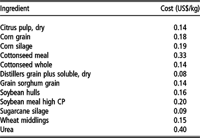
We use bioeconomic data based on a representative feedlot finishing system in Brazil (ANUALPEC, 2017) consisting of Nellore steers with average BCS 5 and the initial SBW of 300 kg under a finishing time of 60 days. Table 1 shows the used ingredients and costs (CEPEA, 2018). Nellore selling price S was assumed 1.44 (US$/kg) (CEPEA, 2018). We obtained the ingredient’s properties from the NASEM (2016) feed library, presented in Supplementary Table S1.
Table 1 Common Brazilian ingredients used in ration formulation (CEPEA, 2018) for Nellore beef cattle
Results
Figure 2 shows the profit, diet cost and SWG as a function of CNEm for the maximum profit model. Figure 2 shows that the optimal solution for CNEm (1.88 Mcal/kg) does not coincide with maximum SWG nor with minimum diet cost. The plotted range CNEm = [0.8, 1.95] is defined by the NLP feasibility, that is, for all values outside this range, the problem is unfeasible. Note that there are slight changes in the curve inflection (∂f/∂CNEm) in similar positions for all three curves. Figure 3 shows how diet profiles vary for different values of CNEm. The black line indicates the maximum profit solution, and the white lines divide regions where a change in inflection occurs. We identify those occurrences by the dual values, that is, indicators of activity of each constraint, and reduced costs, that is, an indicator of minimal change in each variable coefficient to change optimal solution.

Figure 2 Results from the parametric linear programming algorithm for the profit-maximizing diet model for beef cattle. The green dots represent maximum daily profit (US$/day) for that concentration of net energy for maintenance (CNEm (Mcal/kg)), calculated as shrunk-weight gain (kg/day) (SWG – blue triangle) times animal’s sale price, minus daily costs (US$/day) (daily cost – yellow rhombus). The white markers represent the optimal solution, that is, maximum daily profit.

Figure 3 Diet profiles for the concentration of net energy for maintenance (CNEm) (Mcal/kg) range (0.8, 1.95) for the profit-maximizing diet model for beef cattle. The black line highlights the diet profile of the nonlinear programming model optimal solution. The white lines mark a change in the constraints activity.
Figure 2 also shows that diet cost decreases in direction to CNEm = 1.62 (Mcal/kg). For CNEm < 1.29 (Mcal/kg), this is mostly because of the reduction in urea concentration in the diet, as we see in Figure 3. Urea is used as a protein source and is one of the most expensive ingredients available. But the limited allowance of energetic concentration promotes the use of urea as a protein source. As CNEm increases, cheaper feedstuff replacements increase contribution to protein requirements. For 1.29 ≤ CNEm ≤ 1.62, the increased allowance permits the inclusion of distillery grains, which are rich in fat.
For CNEm = 1.28 (Mcal/kg), we observe a jump in SWG and cost in Figure 2. This subtle change coincides with the white line in Figure 3. Once the shift in inflection comes from the change in the constraints activity, it is expected that such bumps in the function may happen in the parameters. For CNEm ≥ 1.64 (Mcal/kg), the increase in profit derives mainly from an increase in SWG as the diet cost keeps increasing steadily after this point. Figure 3 shows that as CNEm increases in this range, the diet changes the ratio of sugarcane silage to sorghum grain and whole cottonseed. This shift is a response to the increase in required protein to achieve higher SWG since those ingredients have more than twice the amount of proteins of sugarcane silage.
In the analysis, all diets formulated for CNEm ≤ 1.56 (Mcal/kg) have a negative profit. However, all diets formulated for 1.85 ≤ CNEm ≤ 1.94 have very similar profit margins and the same five ingredients in their composition: urea, sugarcane silage, cottonseed whole soybean meal high CP and sorghum grain. In that interval, RDP and peNDF requirements are the only active constraints, suggesting that the presence of sugarcane silage in the diet is only used to control ruminal pH.
For CNEm ≥ 1.94, dual values are 0 for metabolized protein constraint and ∑j∈J cnemjx j=CNEmi, so at this point, protein requirements are easily met but the increase in SWG per CNEm no longer increases daily profit, which starts to decrease faster from this point. Beyond this point, there are no combinations of ingredients that can satisfy ∑j∈J cnemjx j = CNEmi, particularly because only four ingredients contain cnemj> 1.94, and none of those contain forage to satisfy the peNDF constraint.
The optimal diet is at CNEm = 1.88 Mcal/kg and DMI of 6.85 kg/day containing 20.21% of cottonseed whole, 39.62% of sorghum grain, 22.26% of soybean meal high CP, 14.24% of sugarcane silage and 3.67% of urea. The daily profit of US$0.41/day is associated with a SWG of 1.21 kg/day and a diet cost of US$1.33/day.
Figure 4a shows the normalized solution for three different objective functions: minimum cost, maximum profit and maximum profit/SWG. Figure 4b shows the optimal diet composition for the different objective functions. Figure 4a indicates that using the up-to-date NASEM (2016) the different objective functions are not equivalent, once the optimal solutions highlighted are at different CNEm values. Analyzing daily profit for those optimal solutions indicates that it is 9.1% lower for the maximum profit/SWG and 52.3% lower for the minimum cost, compared to the maximum profit objective function. Figure 4b also shows that the optimal diet composition for each objective differs significantly.

Figure 4 Results of different objective function of the profit-maximizing diet model for beef cattle. (a) Comparison of different normalized objective functions: maximum daily profit, maximum profit per shrunk weight gain (SWG) and minimum cost for the range of concentration of net energy for maintenance (CNEm). For each objective function, the optimal solution is highlighted in white. The normalization converts the optimal value to 1 and −1 for maximization and minimization problems, respectively. (b) Diet profile of the optimal solutions for the different objective functions in (a).
Sensitivity analysis of the optimal solution shows that, for unused ingredients, the decrease in price (US$/kg) necessary to change the diet composition is US$0.10 for citrus pulp, US$0.10 for corn grain, US$2.17 for corn silage, US$1.20 for cottonseed meal, US$0.18 for distillers grain, US$0.70 for soybean hull and US$0.41 for wheat middlings. High values in some of these ingredients indicate that they are not competitive enough to be a viable replacement.
Sensitivity analysis on the BCS, SBW and S indicates that profit can increase with lower BCS or SBW, as well as with higher S (see Supplementary Table S2). Once the increase in SBW and BCS influences the energy and protein requirements while reducing SWG, it is expected that larger profit margins come from fattening smaller animals. From the selling price sensitivity, we see that higher prices correlate with more energetically concentrated diets. This behavior possibly indicates the existence of a trade-off point where the extra profit margin is larger than the cost of feeding and attending minimum nutritional requirements. Moreover, in every sensitivity scenario all optimal diets contain the same five ingredients in different proportions: cottonseed whole (18.74% to 22.28%), sorghum grain (12.88% to 58.67%) of soybean meal high CP (0.00% to 53.49%), sugarcane silage (11.35% to 16.299%) and urea (0.00% to 6.29%).
We show in Figure 5 the convergence results using numerical optimization with precision ε = 10−2. The GSS takes O(log ε−1) iterations to complete. Daily profit and CNEm converged for the same optimal values found using the brute force search: US$0.41/day and 1.88 Mcal/kg. While the brute force algorithm took 114 iterations to find the optimal solution with ε = 10−2, the GSS took 10 for the same ε. Since the number of iterations to find a solution through brute force in a range D is n = ⌈D 2/ε⌉, for ε =10−6 and D = 1.15, it would require 1 322 500 iterations. On the other hand, for the same range D, the GSS would need n = ⌈(log ε − log D)/log ϕ⌉, that is, 29 iterations for ε = 10 −6. In terms of computational time, the brute force algorithm took 2.120 s, while the GSS algorithm took 1.150 s, both for the precision of ε =10−2. We estimate that most of this time was spent in overhead.

Figure 5 Golden-section search algorithm of the profit-maximizing diet model for beef cattle. Results show convergence for daily profit (blue dot) and concentration of net energy for maintenance (CNEm – red rhombus).
Discussion
Transforming the NLP problem into a parametric LP equivalent has practical and computational advantages. Since LPs can be solved in pseudo-polynomial time, we have a good estimation of computational time based solely on a few characteristics of the data and model. The brute force search algorithm is the slowest possible approach, having to solve O(ε−1) LPs to find the ε-solution for the NLP model. However, it is unrealistic to work with precisions greater than 10−2 in diet formulation, which means a solution can usually be found with no more than 200 LPs resolutions, depending on the feasible range of CNEm. Once this diet optimization model is small, that is, 7 constraints and no more than 300 feed ingredients in NASEM (2016)’s library, it can be further developed for more complex scenarios, for example, environmental constraints, where the GSS approach can be more relevant in terms of execution time.
The proposed approach has advantages compared to the traditional least-cost diet alternative. An arbitrary choice of CNEm may lead to suboptimal solutions, including no profit scenarios. Thus, using parametric LP to solve the least-cost model for the whole feasible CNEm interval can improve the solution compared to the traditional approach. However, it can also lead to a suboptimal solution in terms of profit, that is, revenue minus costs. We also show that the assumption that maximum profit per SWG is equivalent to maximum profit is invalid when using the most updated predictive equations (NASEM, 2016).
The GSS showed a significant increase in performance compared with the brute force search. For ε =10−2, it took 10 iterations to complete, roughly 1/10 of the initial approach. Since the GSS has to solve only O(log ε−1) LPs, it can be useful for more complex diet optimization models. Empirical evidence shows that the function Z(CNEm, x) on Equation (23) is unimodular; thus, both brute force and GSS are guaranteed to obtain a minimizer within ε of that exact minimizer.
Further model limitations are related to the assumed linear growth of SBW over time. Since the predicted requirements change with cattle bodyweight, ideally, the model should revaluate diet periodically. Thus, the results will accumulate greater inaccuracy from the dynamic weight of the animal, proportionally to the feeding time. This inaccuracy is reflected in the difference in the animal weight curve in time, between the linear approximation of SWG and nonlinear SWG. This measurement can be obtained by solving the differential equation system for growth. To overcome this, the feeding time T can be discretized by a micro-period p to maximize profit along the whole feeding time. Thus, a new index t ∈ {1, …, T/p} can be introduced into the model, with T and p arbitrarily chosen according to the desired precision and computational power. This approach is equivalent to approximate nonlinear growth by multiple linear segments.
Mathematical models to optimize diet are always bounded to limitations on the accuracy of predictive equations for nutrient requirements and absorption. Nevertheless, under the infinite set of possible diets, numerical optimization techniques deliver a ‘close to optimal’ solution facing variation proportional to the uncertainty in the process. Some suggest adjustments on predictive equations based on each particular application (NASEM, 2016), which may also correct the assertiveness of our model’s solution. Still, it is key to have a proper understanding of the premises and scope of both the predictive equations and the mathematical optimization models when applying them to cattle feeding operations. In this sense, the dataset and respective sensitivity analysis on price, SBW and BCS show that the diets for different sale prices (+15% to −15%) contain the same ingredients in different proportions. This sensitivity analysis approach can deliver a local assessment of how much uncertainty in price and SBW can be absorbed, while indicating a range for possible diet formulation. This result indicates that the maximum profit model may contain a degree of robustness for uncertainty, which could be enhanced with the development of a stochastic optimization model for maximum profit.
Furthermore, in response to concerns over livestock emissions, researchers have been focusing on the environmental impacts of rations. Optimization models to evaluate economic and environmental (impact) trade-offs usually modify the traditional least-cost algorithm objective function (Wang et al., Reference Wang, Fox, Cherney, Chase and Tedeschi2000a and Reference Wang, Fox, Cherney, Chase and Tedeschi2000b; Tedeschi et al., Reference Tedeschi, Fox, Chase and Wang2000; Pomar et al., Reference Pomar, Dubeau, Létourneau-Montminy, Boucher and Julien2007; Oishi et al., Reference Oishi, Kumagai and Hirooka2011; Moraes et al., Reference Moraes, Wilen, Robinson and Fadel2012), use multi-criteria analysis (Hadrich et al., Reference Hadrich, Wolf and Harsh2005; Moraes and Fadel, Reference Moraes, Fadel and Kebreab2013; Moraes et al., Reference Moraes, Fadel, Castillo, Casper, Tricarico and Kebreab2015), develop multi-objective models (Garcia-Launay et al., Reference Garcia-Launay, Dusart, Espagnol, Laisse-Redoux, Gaudré, Méda and Wilfart2018) or integrate lifecycle assessment analysis exogenously (Oishi et al., Reference Oishi, Kato, Ogino and Hirooka2013; Mackenzie et al., Reference Mackenzie, Leinonen, Ferguson and Kyriazakis2016). As our results show, the choice of the objective function will impact the optimal solution and hence, the related economic analysis. Thus, results from studies using least-cost models should be reevaluated, at least considering the whole range of CNEm. Moreover, the NASEM (2016) model suggests a variety of equations to predict CH4 emissions. Such equations (e.g. those based on the International Panel on Climate Change guidelines; Eggleston et al., Reference Eggleston, Buendia, Miwa, Ngara and Tanabe2006) can also be introduced into our model either in the constraints or in the objective function.
Conclusion
Our model permits optimal diet formulation by considering the interaction between CNEm, CNEg and diet profit. As the choice of maximum profit, profit/SWG or minimum diet cost leads to different solutions, the objective function must be carefully chosen prior to any economic or policy analysis.
From a nutritional perspective, our model presents a straightforward approach to define a baseline diet solely based on animal characteristics. Since it does not require net energy concentration beforehand, it has a broader solution space than a traditional least-cost diet. Furthermore, the relation with the NASEM (2016)’s prediction system allows the same approximations to be made in our model.
It is unlikely that in the future, the NASEM (2016)’s equations will evolve in a way that compromises our model (Tedeschi, Reference Tedeschi2019) since it would concurrently jeopardize the process by which the nutritionist formulates the baseline diet. Thus, as their system continues to evolve, our model should be able to accommodate changes in the equations for the nutrient requirement prediction either by linearization, subject to an increase in inaccuracy, or through parametrization of nonlinear factors.
The parametric LP approach makes it easier to implement further developments to the model to asses a more complex situation. Furthermore, the possibility of solving the profit-maximizing diet problem with the GSS suggests that our model could be extended or integrated with others, and still be solved efficiently.
Acknowledgements
This work was supported by The University of Edinburgh’s Data-Driven Innovation Chancellors fellowship. We also acknowledge the Economic and Social Research Council (ESRC) under grant number ES/N013255/1 and CAPES Foundation for the scholarship no. 10180/13-3.
J. G. O. Marques 0000-0002-4099-085X
R. de O. Silva 0000-0003-3440-580X
L. G. Barioni 0000-0003-1716-1428
J. A. J. Hall 0000-0002-0030-013X
L. O. Tedeschi 0000-0003-1883-4911
D. Moran 0000-0001-8147-5742
Declaration of interest
None.
Ethics statement
Not applicable.
Software and data repository resources
The mathematical model programmed in Python 3, including the dataset used in this work, is available in the GitHub repository at Marques (Reference Marques2020) under GNU General Public License v3.0.
Supplementary material
To view supplementary material for this article, please visit https://doi.org/10.1017/S1751731120001433


