


1 Introduction
With the rise of digital economy, cyber risk has become a major concern for all customer segments. Most research programs on cyber risk focus mainly on cyber security and physical means, in view of developing protection against hacking and data breaches. Although the development of such strategies is fundamental, no protection is perfect and insurers are intended to play a crucial role in providing financial protection. This explains the expansion of cyber insurance contracts.
In the meantime, few works exist on the consequences of cyber attacks from an insurance point of view, and the scientific literature on pricing and reserving of cyber insurance contracts is not very vast. Topics recently addressed in cyber insurance are reviewed in Biener et al. (Reference Biener, Eling and Wirfs2015), Eling & Schnell (Reference Eling and Schnell2016) or Marotta et al. (Reference Marotta, Martinelli, Nanni, Orlando and Yautsiukhin2017). Most of the work on cyber insurance comes from the field of computer science, or from the economic science. For instance, in the field of computer science, Fahrenwaldt et al. (Reference Fahrenwaldt, Weber and Weske2018) study the topology of infected networks, and Rios et al. (2019) gather expert judgements using an adversarial risk analysis. Noel et al. (Reference Noel, Jajodia, Wang and Singhal2010) and Homer et al. (Reference Homer, Zhang, Ou, Schmidt, Du, Raj Rajagopalan and Singhal2013) consider a modelling through attack graphs to measure the security risk of networks (in Noel et al. Reference Noel, Jajodia, Wang and Singhal2010) or to propose an aggregating vulnerability metrics for enterprise networks (in Homer et al. Reference Homer, Zhang, Ou, Schmidt, Du, Raj Rajagopalan and Singhal2013). Johnson et al. (Reference Johnson, Böhme and Grossklags2011) provide analytical models of security games to compute adjusting incentives in order to improve network security. In the field of economic science, one may mention the contributions of Böhme and his co-authors, such as Böhme & Kataria (Reference Böhme and Kataria2006), Böhme & Schwartz (Reference Böhme and Schwartz2010), Riek et al. (Reference Riek, Böhme, Ciere, Ganan and van Eeten2016). Saini et al. (Reference Saini, Azad, Raut and Hadimani2011) use the utility theory to compute an insurance premium for cyber risk insurance, while a gametheoric approach is proposed by Wang et al. (Reference Wang2019), who investigate a mix between optimal investments in information security and cyber insurance innovation.
Herath & Herath (Reference Herath and Herath2011), Eling & Loperfido (Reference Eling and Loperfido2017) and Farkas et al. studied statistical properties and developed more established insurance modelling methods illustrated on the Privacy Rights Clearinghouse (PRC) database. This database has also been studied by Maillart et al. (2010) to quantify the distribution and time evolution of cyber risks, and by Edwards et al. (Reference Edwards, Hofmeyr and Forrest2016) who developed Bayesian Generalised Linear Models to investigate trends in data breaches. This public data set is considered as a benchmark for cyber event analysis.
This paper puts this data set at the cornerstone of the evaluation approach, using statistical techniques to model dynamic dependence and evolving events and providing an operational tool for insurance companies to quantify cyber risk. It takes into account the evolution of the information, while also quantifying the uncertainty of predictions. This is all the more important given that the threat of cyber risk is rapidly growing and evolving, making it one of the most important social and economic risks.
The modelling of cyber attacks frequency requires to take account of complex dependence effects since the majority of systems have the same flaws and are interconnected. Some works have been done in this direction, as it is the case in Peng et al. (Reference Peng, Xu, Xu and Hu2017) in the cyber security field. In the insurance framework, one can cite Böhme & Kataria (Reference Böhme and Kataria2006) and Herath & Herath (Reference Herath and Herath2011) for a model using copulas; another possible approach is to use network contagion models, as in Xu & Hua (Reference Xu and Hua2019). Due to the presence of accumulation phenomena and contagion, the use of Hawkes processes to understand the frequency of the claims will be proposed. Baldwin et al. (Reference Baldwin, Gheyas, Ioannidis, Pym and Williams2017) claim that Hawkes processes provide the adequate modelling of cyber attacks into information systems because they capture both shocks and persistence after shocks that may form attack contagion. These processes, through their self-exciting property, are adapted to model aftershocks of cyber attacks.
In this paper, we propose to use Hawkes processes, motivated by applications in the field of insurance, including pricing and solvency capital requirement calculation. Hawkes processes have been introduced in Hawkes (Reference Hawkes1971), and they have the peculiarity to model excitation effects. Historically, there was a first boom in their application in seismology, since then they have been widely used in many different fields, among which finance, neurology, population dynamics or social network modelling. Amongst the recent papers, one can cite, for instance, Boumezoued (Reference Boumezoued2016) for population dynamics modelling, Embrechts et al. (Reference Embrechts, Liniger and Lin2011), Bacry et al. (Reference Bacry, Mastromatteo and Muzy2015) and Hainaut (Reference Hainaut2016) in finance, Errais et al. (Reference Errais, Giesecke and Goldberg2010) in credit risk, Stabile & Torrisi (Reference Stabile and Torrisi2010), Jang & Dassios (Reference Jang and Dassios2013) and Barsotti et al. (Reference Barsotti, Milhaud and Salhi2016) in insurance and Rizoiu et al. (Reference Rizoiu, Lee, Mishra and Xie2017) in the field of social media. Such processes have been recently used in the cyber security field, for instance by Baldwin et al. (Reference Baldwin, Gheyas, Ioannidis, Pym and Williams2017) who studied the self- and mutually exciting properties of the threats to 10 important IP services, using industry standard SANS data or by Peng et al. (Reference Peng, Xu, Xu and Hu2017) who focused on extreme cyber attacks rates. Up to our knowledge, Hawkes processes have not been already used to model cyber attacks in the insurance framework. This paper proposes to study the application of these processes on the public PRC database, which makes a census of data breaches happening in the United-States.
In addition to the fact that computer systems are interconnected between companies and that attacks may be driven by common sources, two statistical arguments motivate our choice to use Hawkes processes. The first one is the rejection of the Poissonian hypothesis. Indeed, a Kolmogorov–Smirnov test for the suitability of the inter-arrival times to an exponential distribution leads to a clear rejection with a p-value close to zero. The second one is the detection of autocorrelation in the number of attacks. Indeed, drawing the number of attacks in a month
 $t+1$
as a function of the number of attacks in a month t, by type of attacks, leads to a correlation coefficient of 65%; this is depicted in Figure 1.
$t+1$
as a function of the number of attacks in a month t, by type of attacks, leads to a correlation coefficient of 65%; this is depicted in Figure 1.
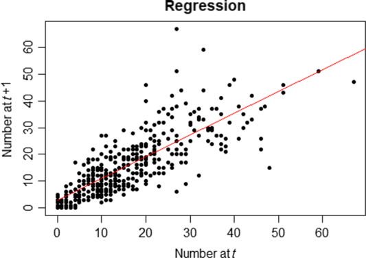
Figure 1 Regression of the number of 1-month attacks on the previous one – by type of attacks –
 $R^2=0.6548$
.
$R^2=0.6548$
.
To reproduce autocorrelation between inter-arrival times, two natural choices are the Cox processes and the Hawkes processes (see, e.g. Daley & Vere-Jones (Reference Daley and Vere-Jones2007) for a survey on point processes). In Cox processes (also known as doubly stochastic Poisson processes), the autocorrelation is captured through the time-dependent intensity that is itself a stochastic process. However, the appropriate specification of the stochastic intensity dynamics remains challenging. Therefore, we resort to the class of Hawkes self-exciting processes which benefit from an interpretable and rather parsimonious parametric representation. In addition to autocorrelation, the Hawkes processes allow to take into account excitation effects, by making arrival rate of events depends on the past events. This seems to make sense in the context of cyber risk, for example, a software flaw discovered will probably generate many attacks in a short time. Another example is the contagion of a virus on other computers, for instance, the ransomware Wannacry attack in 2017, that led to a contagion of more than 300,000 computers over more than 150 countries.
In this paper, we propose a stochastic modelling to analyse and predict the arrivals of cyber events. The study is carried out on the PRC database. We specify and infer multivariate Hawkes processes with specific kernel choices to model the dynamics of data breaches times, depending on their characteristics (type, target and location). This modelling framework allows for a causal analysis of the autocorrelation between inter-arrival times according to each data breach feature and provides forecasts of the full joint distribution of the future times of attacks. This is a first step in the actuarial quantification of cyber risk, more especially on its frequency component. Nevertheless, it is almost impossible to know from the PRC database which part of the variation along time of the reported claims is caused by an evolution of the risk, and which part is caused by an instability in the way the data are collected. Indeed, to fully capture the frequency component, one should also have information about the exposure. However, capturing this component remains challenging since one should track the number of entities by sector exposed to cyber risk over time, along with ensuring the exhaustiveness of the claims reporting process within the PRC data set. That is why the exposure quantification will not be addressed in this work. Concerning the severity component, the PRC data set provides a proxy in terms of the number of records breached for each event. This variable is expected to be strongly correlated with the real loss of the event. Nevertheless, the standard formulas used to deduce a loss from the number of breached records are questionable, such as Jacobs formula (Jacobs Reference Jacobs2014) proposed in Reference Jacobs2014 (using data gathered by Ponemon Institute for the publication of the 2013 and 2014 Cost of Data Breach), which has been recently updated by Farkas et al. Again, a better assessment of the severity risk would require information about the characteristics of the type of breach and of the breached entity, and that are not available on the PRC database.
The remainder of this paper is as follows. In section 2, we describe the data breach data set from the PRC and the classification of data breach features as used in this study. Section 3 describes the multivariate Hawkes modelling framework, the kernel specifications considered as well as the likelihood. The main inference and prediction results are detailed in section 4, while our supporting results on the closed-form expectation of the multivariate Hawkes model are given in Appendix B.
2 Data Set
The analysis is based on the data set from the PRC that is described below, as well as different classes of data breach that will be considered.
Table 1. Type of breaches – origin refers to the PRC classification – aggregation refers to our classification.

2.1 Description
The data set from the PRC Footnote 1 contains 8,871 data breaches which have been made public since 2005. Our study focuses on the period 2010–2019, to avoid too much heterogeneity in the type of sources reporting the cyber breaches to the PRC data set. Indeed, although data breach notification laws have been enacted at different dates in different states, many of them were enacted before 2010; therefore, we decided to study the database from this date. For each breach, the following information is available:
-
• name of the covered entity;
-
• type of the covered entity;
-
• localisation of the breached entity;
-
• breach submission date;
-
• type of breach;
-
• number of individuals affected;
-
• localisation of the breached information;
-
• source of information (US Government Agencies, non-profit organisations, media…).
In Table 1, we present the classification of the types of breaches within the PRC (column “Origin”), as well as our preliminary aggregation as used in this paper (column “Aggregation”), which will be further discussed in section 4. The main types of breaches and entities recorded in the data set are depicted in Figures 2 and 3.
Figure 2 shows three main categories that contain around 75.7% of the data. One can also remark the high level of unintended disclosure (21.1%) and non-electronic data (21.8%).
Table 2. Type of organisation breached – origin refers to the PRC classification – aggregation refers to our classification.
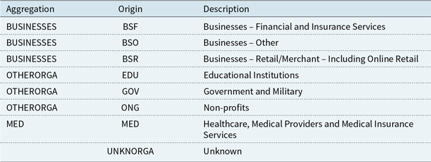

Figure 2 PRC types of breaches.

Figure 3 PRC types of organisations breached.
The Healthcare industry seems to experience far more breaches than others, even than the Businesses, despite they have a lower exposure in terms of number of entities. It may be explained by the fact that personal health information is often more valuable on the black market than other data as it is the case for credit card credentials. The second industry mainly targeted is the businesses. The PRC classification as well as our own aggregation is depicted in Table 2.
In Appendix A, the table with the number of breaches reported in each state shows a clear heterogeneity. While California counts more than 15% of the total data available, many states such as Alabama or Arkansas are under 1%. This fact could be linked with the age of the notification law in each state as well as the exposure in terms of number of entities at risk.
2.2 Aggregation
In order to get larger groups for the following study, we decided to group the attack types according to their similarities, see Table 1. The types PHYS, PORT and STAT are gathered in a new category named Theft/Loss. In the same way, we grouped CARD and INSD in a new category named Other. These categories represent, respectively, 32.3% and 7.5% of the database.
Concerning the organisation types, with the same arguments, we grouped BSF, BSO and BSR in a category named BUSINESSES. NGO, EDU and GOV are put in a OtherOrga category. It leads to a representation of 25.5% and 12.8% of the total database; these are detailed in Table 2.
Finally, because of the high heterogeneity of the number of breaches reported in each state, we made a main group named OtherStates (71.1%) and kept the three biggest ones, namely, California (15.7%), Texas (6.9%) and New-York (6.3%).
This granularity which has been derived at this stage of the analysis will be further discussed and aggregated in Section 4.
3 Multivariate Hawkes Model
A multivariate Hawkes framework is proposed to model the clustering and autocorrelation of times of cyber attacks in different groups. In this section, we present the model and the kernel specifications, and we compute the likelihood.
3.1 Model specification
To fix the idea, we recall briefly the definition and main properties of a Hawkes process. A standard (one-dimensional) Hawkes process
 $(N_t)_{t\geq 0}$
is a self-exciting point process defined by its intensity function
$(N_t)_{t\geq 0}$
is a self-exciting point process defined by its intensity function
 $(\lambda_t)_{t\geq 0}$
characterised by a baseline intensity
$(\lambda_t)_{t\geq 0}$
characterised by a baseline intensity
 $(\mu_t)_{t\geq 0}$
plus a self-exciting part
$(\mu_t)_{t\geq 0}$
plus a self-exciting part
 $ \sum_{T_n < t} \phi(t-T_n),$
where
$ \sum_{T_n < t} \phi(t-T_n),$
where
 $T_n$
is the jump time number n, and
$T_n$
is the jump time number n, and
 $\phi$
is a function which governs the clustering density of
$\phi$
is a function which governs the clustering density of
 $(N_t)_{t\geq 0}$
, also called the excitation function or kernel of the Hawkes process. Recall that the intensity
$(N_t)_{t\geq 0}$
, also called the excitation function or kernel of the Hawkes process. Recall that the intensity
 $(\lambda_t)_{t\geq 0}$
represents the “instantaneous probability” to have a jump at time t, given all the past. This basically means that there is a baseline rate
$(\lambda_t)_{t\geq 0}$
represents the “instantaneous probability” to have a jump at time t, given all the past. This basically means that there is a baseline rate
 $(\mu_t)_{t\geq 0}$
to have a spontaneous jump at t but that also all the previous jumps influence the apparition of a jump at t. The existence (using Picard iteration) and the construction (using a thinning procedure) of such processes can be found in Brémaud & Massoulié (Reference Brémaud and Massoulié1996), Brémaud & Massoulié (Reference Brémaud and Massoulié2002). One could also find in Daley & Vere-Jones (Reference Daley and Vere-Jones2007) the main definitions, constructions and models related to point processes in general and Hawkes processes in particular.
$(\mu_t)_{t\geq 0}$
to have a spontaneous jump at t but that also all the previous jumps influence the apparition of a jump at t. The existence (using Picard iteration) and the construction (using a thinning procedure) of such processes can be found in Brémaud & Massoulié (Reference Brémaud and Massoulié1996), Brémaud & Massoulié (Reference Brémaud and Massoulié2002). One could also find in Daley & Vere-Jones (Reference Daley and Vere-Jones2007) the main definitions, constructions and models related to point processes in general and Hawkes processes in particular.
In what follows, a multivariate Hawkes process is considered to capture the clustering and the autocorrelation between inter-arrival times, according to each data breach feature. We consider d groups of data breaches; these groups can be defined by crossing the several covariate dimensions as described in section 2. For example, a given group can relate to data breaches of
-
• the same type (e.g. THEFT/LOSS);
-
• towards same entities (e.g. MED);
-
• in same location (e.g. California).
We consider a time origin at zero being set as the beginning of the first year of the historical period. From this time, data breaches occur in each group
 $i \in \{1,...,d\}$
at random times denoted by
$i \in \{1,...,d\}$
at random times denoted by
 $(T_n^{(i)})_{n\geq 1}$
. This sequence defines a counting process
$(T_n^{(i)})_{n\geq 1}$
. This sequence defines a counting process
 $(N^{(i)}_t)_{t\geq 0}$
as
$(N^{(i)}_t)_{t\geq 0}$
as
 \begin{equation*}N^{(i)}_t=\sum_{n\geq 1} {\mathbf{1}}_{T^{(i)}_n\leq t}\end{equation*}
Therefore,
 $N^{(i)}_t$
is the number of data breaches which occurred for group i in the time interval [0, t]. The intensity process of
$N^{(i)}_t$
is the number of data breaches which occurred for group i in the time interval [0, t]. The intensity process of
 $(N^{(i)}_t)_{t\geq 0}$
is denoted by
$(N^{(i)}_t)_{t\geq 0}$
is denoted by
 $(\lambda_t^{(i)})_{t\geq 0}$
.
$(\lambda_t^{(i)})_{t\geq 0}$
.
We propose a Hawkes process to model the self-excitation in each group as well the excitation between groups. It is specified as follows.
-
• For each
 $i\in\{1,...,d\}$
, the base intensity is a deterministic, continuous and non-negative map
$t \mapsto \mu_t^{(i)}$
.
$i\in\{1,...,d\}$
, the base intensity is a deterministic, continuous and non-negative map
$t \mapsto \mu_t^{(i)}$
. -
• For each
$(i,j)\in\{1,...,d\}^2$
, self- and mutually exciting maps
$t \mapsto \phi_{i,j}(t)$
(commonly called kernels) are introduced and also assumed to be deterministic, continuous and non-negative. -
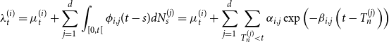
• For each
$i\in\{1,...,d\}$
, the intensity process of
$(N^{(i)}_t)_{t\geq 0}$
is specified as follows: (1)
\begin{equation}\lambda_t^{(i)}=\mu_t^{(i)}+\sum_{j=1}^d \sum_{T_n^{(j)}
< t} \phi_{i,j}\left(t-T_n^{(j)}\right)=\mu_t^{(i)}+\sum_{j=1}^d \int_{[0,t[} \phi_{i,j}(t-s) {{d}} N_s^{(j)}\end{equation}


In this model, the maps
 $\phi_{i,i}$
quantify the self-excitation in the group i, whereas for
$\phi_{i,i}$
quantify the self-excitation in the group i, whereas for
 $i\neq j$
, the map
$i\neq j$
, the map
 $\phi_{i,j}$
quantifies the contagion in group i caused by a data breach in group j. Note here that each intensity process
$\phi_{i,j}$
quantifies the contagion in group i caused by a data breach in group j. Note here that each intensity process
 $\lambda^{(i)}$
is adapted to the canonical filtration associated with the whole set of processes
$\lambda^{(i)}$
is adapted to the canonical filtration associated with the whole set of processes
 $(N^{(j)})_{j\in \{1,...,d \}}$
; in this way, the behaviour of a given group may (generally) depend on that of the others.
$(N^{(j)})_{j\in \{1,...,d \}}$
; in this way, the behaviour of a given group may (generally) depend on that of the others.
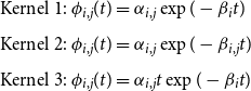
The framework of interest in this paper is made of the two following kernels specifications:
 \begin{eqnarray}
\phi_{i,j}(t) & = & \alpha_{i,j} \exp \left( - \beta_{i,j} t\right)\nonumber\\
\phi_{i,j}(t) & = & \alpha_{i,j}t \exp \left( - \beta_{i,j} t\right)\end{eqnarray}
\begin{eqnarray}
\phi_{i,j}(t) & = & \alpha_{i,j} \exp \left( - \beta_{i,j} t\right)\nonumber\\
\phi_{i,j}(t) & = & \alpha_{i,j}t \exp \left( - \beta_{i,j} t\right)\end{eqnarray}
Examples of such kernels are provided in Figure 4. The first one models an instantaneous excitation when an event occurs, and then it decreases exponentially towards zero. It is the most widely used in the literature as it allows the intensity to be Markovian in the univariate case, as well as in the multivariate setting under some restrictions, see the next remark. The second one models a progressive excitation that reaches its highest level after a time
 $1/\beta_{i,j}$
, after this, the impact decreases towards zero.
$1/\beta_{i,j}$
, after this, the impact decreases towards zero.

Figure 4 Evolution of kernels through time.
Remark 1. Although other forms of kernels can be considered (see, e.g. Boumezoued (Reference Boumezoued2016) for the computation of Hawkes distribution for general kernel assumptions), we restrict here our attention to these cases; extension to other kernels encompassing more parameters and related optimal selection is left for further research. Note that this framework is still rich enough. Indeed, the Hawkes process intensity is not Markov with the specification
 $\phi_{i,j}(t)=\alpha_{i,j}t \exp \left( - \beta_{i,j} t\right)$
. Moreover, for the exponential specification
$\phi_{i,j}(t)=\alpha_{i,j}t \exp \left( - \beta_{i,j} t\right)$
. Moreover, for the exponential specification
 $\phi_{i,j}(t)=\alpha_{i,j} \exp \left( - \beta_{i,j} t\right)$
with parameters
$\phi_{i,j}(t)=\alpha_{i,j} \exp \left( - \beta_{i,j} t\right)$
with parameters
 $\beta_{i,j}$
depending on the interacting groups i and j, the vector
$\beta_{i,j}$
depending on the interacting groups i and j, the vector
 $(\lambda^{(1)},...,\lambda^{(d)})$
of the Hawkes intensity processes is not Markov; it is only the case when for any i all the
$(\lambda^{(1)},...,\lambda^{(d)})$
of the Hawkes intensity processes is not Markov; it is only the case when for any i all the
 $\beta_{i,j}$
are constant equal to some
$\beta_{i,j}$
are constant equal to some
 $\beta_i$
, that is when the memory of impacts from a group j on a group i only depends on group i. These general frameworks will lead us to consider an extended process with additional well chosen components to recover a higher dimensional dynamics and tractable formulas, see Appendix B. Finally, recall that the multivariate Hawkes process
$\beta_i$
, that is when the memory of impacts from a group j on a group i only depends on group i. These general frameworks will lead us to consider an extended process with additional well chosen components to recover a higher dimensional dynamics and tractable formulas, see Appendix B. Finally, recall that the multivariate Hawkes process
 $(N^{(1)},...,N^{(d)})$
is not Markov in both parametrisations.
$(N^{(1)},...,N^{(d)})$
is not Markov in both parametrisations.
3.2 Likelihood
The aim of this section is to detail the likelihood of the multivariate Hawkes model. This likelihood is known as for any counting process with stochastic intensity and can be found in related references such as Ozaki (Reference Ozaki1979); we still provide its computation here for sake of completeness. Note that we implement a “brute force” multidimensional optimisation for maximum likelihood estimation (using the “Nelder-Mead” algorithm from the “optim” function in R). There exists alternatives to this approach, for example, using a stochastic descent algorithm, see Jaisson (Reference Jaisson2015) and Bacry et al. (Reference Bacry, Mastromatteo and Muzy2015) for a general discussion on inference strategies in a high-dimensional framework in the context of financial applications. Let us consider that the processes are observed on a given interval
 $[0,\tau]$
.
$[0,\tau]$
.
Proposition 1. The log-likelihood of a multidimensional Hawkes process
 $\big(N^{(i)}\big)_{1\leq i \leq d}$
with baseline intensity
$\big(N^{(i)}\big)_{1\leq i \leq d}$
with baseline intensity
 $\big(\mu^{(i)}\big)_{1\leq i \leq d}$
and kernels
$\big(\mu^{(i)}\big)_{1\leq i \leq d}$
and kernels
 $\big( \phi_{i,j}(t) = \alpha_{i,j} \exp\left(- \beta_{i,j} t \right)\big)_{ 1\leq i,j \leq d}$
is
$\big( \phi_{i,j}(t) = \alpha_{i,j} \exp\left(- \beta_{i,j} t \right)\big)_{ 1\leq i,j \leq d}$
is
 \begin{eqnarray}
\log \mathcal{L} & = & - \sum_{i = 1}^{d} \int_{0}^\tau (\mu_s^{(i)}+\sum_{j=1}^d \int_0^s \alpha_{i,j} \exp\left(- \beta_{i,j} (s - u) \right) {{d}} N_u^{(j)}) {{d}} s\nonumber \\[5pt]
&& + \sum_{i = 1}^{d} \sum_{n =1}^{m_i} \log \left( \mu^{(i)}_{t^{(i)}_n} +\sum_{j=1}^d \int_0^{t^{(i)}_{n}} \alpha_{i,j} \exp\left(- \beta_{i,j} (t^{(i)}_{n} - s) \right) {{d}} N_s^{(j)} \right)\end{eqnarray}
\begin{eqnarray}
\log \mathcal{L} & = & - \sum_{i = 1}^{d} \int_{0}^\tau (\mu_s^{(i)}+\sum_{j=1}^d \int_0^s \alpha_{i,j} \exp\left(- \beta_{i,j} (s - u) \right) {{d}} N_u^{(j)}) {{d}} s\nonumber \\[5pt]
&& + \sum_{i = 1}^{d} \sum_{n =1}^{m_i} \log \left( \mu^{(i)}_{t^{(i)}_n} +\sum_{j=1}^d \int_0^{t^{(i)}_{n}} \alpha_{i,j} \exp\left(- \beta_{i,j} (t^{(i)}_{n} - s) \right) {{d}} N_s^{(j)} \right)\end{eqnarray}
where
 $(t_n^{(k)})_{1\leq n \leq m_k}$
are the
$(t_n^{(k)})_{1\leq n \leq m_k}$
are the
 $m_k$
times of event observed for each group
$m_k$
times of event observed for each group
 $k \in \{1,...,d\}$
.
$k \in \{1,...,d\}$
.
Proof of Proposition 1.
-
(i) For ease of presentation, let us start with the single group case (
$d=1$
); we omit the group index for simplicity of notation. Note that calibrating such model on each single group amounts to specify
$\phi_{i,j}\equiv 0$
for
$i \neq j$
in Equation (1). We introduce the notation
$\mathcal{H}_n=\{T_n=t_n,...,T_1=t_1\}$
the information on the first n times of event and add the conventions
$\mathcal{H}_0=\emptyset$
and
$T_0=0$
. Having observed the times
$(t_n)_{1\leq n \leq m}$
, the likelihood can be written as (by abuse of notation we keep the
$T_n$
):
Then the log-likelihood can be written as
\begin{equation*}\begin{split}\mathcal{L}&={\mathbb{P}}(\forall 1\leq n \leq m, T_n=t_n, \text{ and } T_{m+1}>\tau)\\[5pt]
&={\mathbb{P}}( T_{m+1}>\tau \mid \mathcal{H}_m ) \prod_{n =1}^m {\mathbb{P}}(T_n=t_n \mid \mathcal{H}_{n-1})\\[5pt]
&=\exp \left( - \int_{T_m}^\tau \lambda_s {{d}} s\right) \prod_{n =1}^m \exp \left( - \int_{T_{n-1}}^{T_n} \lambda_s {{d}} s\right) \lambda_{T_n}\\[5pt]
&=\exp \left( - \int_{0}^\tau \lambda_s {{d}} s\right) \prod_{n =1}^m \lambda_{T_n}\end{split}\end{equation*}
(4)This is the standard log-likelihood for any counting process
\begin{equation}\log \mathcal{L}= - \int_{0}^\tau \lambda_s {{d}} s + \sum_{n =1}^m \log \lambda_{T_n}=- \int_{0}^\tau \lambda_s {{d}} s+\int_0^\tau \log \lambda_s{{d}} N_s\end{equation}
$(N_s)_{s \geq 0}$
with intensity process
$(\lambda_s)_{s \geq 0}$
. It now remains to further specify it in the context of the model introduced in Equation (1), as
(5)If we further specify the self-exciting map as
\begin{equation}\log \mathcal{L}= - \int_{0}^\tau \mu_s {{d}} s - \int_{0}^\tau \sum_{T_n
< s} \phi(s-T_n) {{d}} s + \sum_{n=1}^m \log \left( \mu_{T_n}+ \sum_{k=1}^{n-1} \phi(T_n-T_k) \right)\end{equation}
$\phi(t)=\alpha \exp\left( - \beta t\right)$
, with non-negative
$\alpha$
and
$\beta$
in the present context, we obtain
(6)
\begin{eqnarray} \log \mathcal{L}(\mu,\alpha,\beta) & = & - \int_{0}^\tau \mu_s {{d}} s - \alpha \int_{0}^\tau \sum_{T_n
< s} \exp \left(-\beta(s-T_n) \right) {{d}} s\nonumber\\
&& + \sum_{n=1}^m \log \left( \mu_{T_n}+ \alpha \sum_{k=1}^{n-1} \exp \left(-\beta(T_n-T_k) \right) \right)\end{eqnarray}
-
(ii) In the multivariate setting, the parameters for all groups are gathered into a vector
$M(t)=(\mu_t^{(1)},...,\mu_t^{(d)})$
, possibly time dependent, and two
$d\times d$
matrices
$A=\left( \alpha_{i,j} \right)_{1\leq i,j'\leq d}$
and
$B=\left( \beta_{i,j} \right)_{1\leq i,j\leq d}$
. The multivariate intensity is fully specified in Equation (1), and using the same reasoning as above, we can derive the associated log-likelihood based on observation
$((t_n^{(i)})_{1 \leq n \leq m_i})_{1 \leq i \leq d}$
(7)When specifying the self- and mutually exciting maps
\begin{align}
\log \mathcal{L}(M(.), A, B) & = - \sum_{i = 1}^{d} \int_{0}^\tau \lambda_s^{(i)}{{d}} s + \sum_{i = 1}^{d} \sum_{n =1}^{m_i} \log \lambda^{(i)}_{t^{(i)}_n}\nonumber \\[5pt]
& = - \sum_{i = 1}^{d} \int_{0}^\tau \left(\mu_s^{(i)}+\sum_{j=1}^d \int_0^s \phi_{i,j}(s-u) {{d}} N_u^{(j)}\right) {{d}} s \\[5pt]
&\quad + \sum_{i = 1}^{d} \sum_{n =1}^{m_i} \log\left(\mu^{(i)}_{t^{(i)}_n}+\sum_{j=1}^d \int_0^{t^{(i)}_{n}} \phi_{i,j}(t^{(i)}_{n}-s) {{d}} N_s^{(j)}\right)\nonumber\end{align}
$\phi_{i,j}(t) = \alpha_{i,j} \exp\left(- \beta_{i,j} t \right)$
, the final log-likelihood is given by Equation (3).


Remark 2. In this form, the number of parameters to be estimated is
 $2d^2$
, in addition to the number of parameters of the functions
$2d^2$
, in addition to the number of parameters of the functions
 $\big(\mu^{(i)}\big)_{1\leq i \leq d}$
which will be specified in Section 4.
$\big(\mu^{(i)}\big)_{1\leq i \leq d}$
which will be specified in Section 4.
Remark 3. Due to the complexity of the log-likelihood, we resort in this paper to a simplex-type optimisation procedure in the form of the Nelder–Mead algorithm. Furthermore, we provide in our paper the inference of the memory parameters
 $\beta_{i,j}$
in Equation (1), in addition to the self-excitation matrix
$\beta_{i,j}$
in Equation (1), in addition to the self-excitation matrix
 $(\alpha_{i,j})$
. The fact that the
$(\alpha_{i,j})$
. The fact that the
 $\beta_{i,j}$
are often considered as fixed parameters is discussed in Bacry et al. (Reference Bacry, Mastromatteo and Muzy2015).
$\beta_{i,j}$
are often considered as fixed parameters is discussed in Bacry et al. (Reference Bacry, Mastromatteo and Muzy2015).
4 Inference and Prediction
We decided to use the periods 2011–2015 and 2011–2016 for parameter inference, in order to predict the number of attacks for 2016 and 2017, respectively. The 1-year horizon taken here is motivated by applications in internal models for insurance companies, aiming to quantify the 99.5% most adverse 1-year loss related to cyber risk insurance covers. Note that the exclusion of the years 2018 and 2019 from the analysis is motivated by the fact that the database appears to be incomplete for these 2 years, since 2019 is not fully developed, and maybe due to some delays in reporting for year 2018.
4.1 Segmentation
The aim of our study is to calibrate a multivariate Hawkes process on several groups obtained by crossing the covariates: Type of breach and Type of the covered entity and State. These covariates are those discussed in section 2 and Tables 1, 2 and in Appendix Table A. In particular, we use the aggregated covariates as discussed in section 2.2. In order to have sufficiently represented groups, we kept the largest ones and removed others in the OTHER group. We also put the group MED and OTHER and OTHER in the OTHER group because it was to irregular over the period of interest. This is summarised in Table 3.Footnote 2
Table 3. Studied groups.
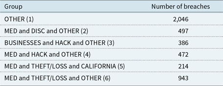
Figure 5 shows the frequency of attacks over the calibration period (2011–2016). First, the different trends strengthen our idea that this segmentation could indeed make sense. These trends will be taken into account through a dedicated linear specification in the baseline intensity. Furthermore, the clustering behaviour of the data breach occurrences appear, alternating high- and low-activity periods, see in particular MED and DISC and OTHER (2) and MED and HACK and OTHER (4).

Figure 5 Numbers of attacks function of the time (in days) for each of the six groups.
4.2 Models studied
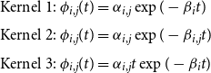
Maximum likelihood inference has been performed for the three following kernels:
 \begin{eqnarray}
&&\text{Kernel 1: } \phi_{i,j}(t) =\alpha_{i,j}\exp(-\beta_{i}t)\nonumber\\[4pt]
&& \text{Kernel 2: } \phi_{i,j}(t) =\alpha_{i,j}\exp(-\beta_{i,j}t)\\[4pt]
&& \text{Kernel 3: } \phi_{i,j}(t) = \alpha_{i,j}t\exp(-\beta_{i}t)\nonumber\end{eqnarray}
\begin{eqnarray}
&&\text{Kernel 1: } \phi_{i,j}(t) =\alpha_{i,j}\exp(-\beta_{i}t)\nonumber\\[4pt]
&& \text{Kernel 2: } \phi_{i,j}(t) =\alpha_{i,j}\exp(-\beta_{i,j}t)\\[4pt]
&& \text{Kernel 3: } \phi_{i,j}(t) = \alpha_{i,j}t\exp(-\beta_{i}t)\nonumber\end{eqnarray}
In order to take into account possible trends in the dynamics, as depicted in Figure 5, a linear baseline intensity
 $(\mu^{(i)}_s)_{s \geq 0}$
has been specified as:
$(\mu^{(i)}_s)_{s \geq 0}$
has been specified as:
 \begin{equation*}\mu^{(i)}_s= \mu^{(i)}_{0}+\gamma_{i} s\end{equation*}
with
 $\mu^{(i)}_{0} \geq 0, \gamma_{i} \in \mathbb{R}$
for
$\mu^{(i)}_{0} \geq 0, \gamma_{i} \in \mathbb{R}$
for
 $i \in \{1,...,d\}$
. Note that in case of a negative trend, the parameters are constrained such that the baseline intensity remains positive at the end of the 1-year forecasting period, that is, for each
$i \in \{1,...,d\}$
. Note that in case of a negative trend, the parameters are constrained such that the baseline intensity remains positive at the end of the 1-year forecasting period, that is, for each
 $i \in \{1,...,d\}$
,
$i \in \{1,...,d\}$
,
 \begin{equation}\mu^{(i)}_{0}+\gamma_{i} (\tau + 1) > 0\end{equation}
This leads, in total, to a number of 54 parameters for kernels 1 and 3, and 84 parameters for kernel 2. Section 4.4 tests a Lasso method to reduce the dimension.
Recall that the first two kernels (exponential case) cause an instantaneous jump of the intensity when an event occur, and then the impact decreases exponentially towards zero (the decrease speed is different for each pair (i, j) in the second case). The third kernel reaches its highest level after a time
 $1/\beta_{i}$
and then the impact decreases towards zero.
$1/\beta_{i}$
and then the impact decreases towards zero.
4.3 Inference
The likelihood obtained through the inference process is provided in Table 4.
Table 4. Opposite of the log-likelihood for each kernel. The largest likelihood are highlighted in bold.

Among the three kernels tested, see Equation (8), it appears that the use of kernel 2 with more parameters provides a better likelihood estimate compared to kernel 1, as expected. However, a key result is that kernel 3 with non-instantaneous excitation provides a better fit than kernel 2, with less parameters. Before detailing the parameter estimates and their interpretation, we present in the following the adequacy test performed.
Adequacy test. We use a statistical test of goodness of fit to evaluate the quality of adjustment of the model. One classical test in the theory of point processes uses the following result, which follows from Theorem 4.1 of Garcia & Kurtz (Reference Garcia and Kurtz2008). Note first that this requires the intensity to remain positive, which is ensured by Equation (9). Remark also that Theorem 4.1 in Garcia & Kurtz (Reference Garcia and Kurtz2008) holds for general counting processes, beyond the class of Hawkes processes.
Proposition 2. Let us define for any
 $i \in \{1,...,d\}$
and
$i \in \{1,...,d\}$
and
 $k\geq1$
,
$k\geq1$
,
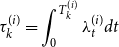 \begin{equation*}\tau_{k}^{(i)}=\int_{0}^{T_{k}^{(i)}} \lambda_t^{(i)} d t\end{equation*}
Then, the
 $(\tau_{k}^{(i)})_{k\geq 1}$
are the jump times of an homogeneous Poisson process of intensity 1.
$(\tau_{k}^{(i)})_{k\geq 1}$
are the jump times of an homogeneous Poisson process of intensity 1.
This result provides a way to test the adequacy of the Hawkes processes: if the underlying process is indeed a Hawkes process with this intensity, the times
 \begin{equation*}\theta_{k}^{(i)} = \tau_{k}^{(i)}-\tau_{k-1}^{(i)}, \text{ } k\geq1\end{equation*}
are independent and distributed according to an exponential distribution with parameter. 1. We can then assess the adequacy for each group
 $i \in \{1,...,d\}$
of the time series
$i \in \{1,...,d\}$
of the time series
 $(\theta_{k}^{(i)})_{k \geq 1}$
to the exponential distribution with a standard Kolmogorov–Smirnov test. This test is based on comparing the distance between the empirical cumulative distribution and that of a reference specified distribution (here exponential) with known parameters (here 1). The adequacy tests for the different kernels are summarised in Table 5. The cases where the null hypothesis (adequacy) is not rejected at confidence level 5 % are highlighted in bold.
$(\theta_{k}^{(i)})_{k \geq 1}$
to the exponential distribution with a standard Kolmogorov–Smirnov test. This test is based on comparing the distance between the empirical cumulative distribution and that of a reference specified distribution (here exponential) with known parameters (here 1). The adequacy tests for the different kernels are summarised in Table 5. The cases where the null hypothesis (adequacy) is not rejected at confidence level 5 % are highlighted in bold.
Table 5. Adequacy test.

From these tests, it appears that the adequacy is satisfactory except for group MED and HACK and OTHER (4), whatever the kernel considered.
Given the quality of the adequacy and of the likelihood presented by kernel 3 (
 $\phi_{i,j}(t) = \alpha_{i,j}t\exp(-\beta_{i}t)$
), we focus on this kernel for the parameter interpretation which follows.
$\phi_{i,j}(t) = \alpha_{i,j}t\exp(-\beta_{i}t)$
), we focus on this kernel for the parameter interpretation which follows.
Parameter estimates – Kernel 3. The parameter estimates for kernel 3 are detailed in Tables 6 and 7; they are interpreted in the following.
Table 6. Parameters
 $(\mu_0^{(i)})_{1\leq i \leq 6}$
,
$(\mu_0^{(i)})_{1\leq i \leq 6}$
,
 $(\beta_{i})_{1\leq i \leq 6}$
and
$(\beta_{i})_{1\leq i \leq 6}$
and
 $(\gamma_{i})_{1\leq i \leq 6}$
.
$(\gamma_{i})_{1\leq i \leq 6}$
.

Table 7. Parameters
 $(\alpha_{i,j})_{1\leq i,j \leq 6}$
.
$(\alpha_{i,j})_{1\leq i,j \leq 6}$
.

To further analyse the parameters, we also compute in Table 8 the maximum value
 $\Gamma_{i,j}$
of the influence of an event of group j on the intensity of the group i (for
$\Gamma_{i,j}$
of the influence of an event of group j on the intensity of the group i (for
 $1\leq i,j \leq d$
). This maximum influence is reached after a certain time, as specified before, up to the value
$1\leq i,j \leq d$
). This maximum influence is reached after a certain time, as specified before, up to the value
 $\Gamma_{i,j}\,\coloneqq \,\frac{\alpha_{i,j}}{\beta_{i}} e^{-1}$
.
$\Gamma_{i,j}\,\coloneqq \,\frac{\alpha_{i,j}}{\beta_{i}} e^{-1}$
.
Table 8. Maximum excitations
 $(\Gamma_{i,\,j})_{1\leq i,\,j \leq 6}$
.
$(\Gamma_{i,\,j})_{1\leq i,\,j \leq 6}$
.

Finally, the ratio
 $\Big(\frac{\Gamma_{i,j}}{\mu_0^{(i)}}\Big)_{1\leq i,j \leq 6}$
between the maximum excitation and the baseline intensity is provided in Table 9. This ratio helps to understand the relative importance of the excitation phenomenon compared to the baseline dynamics.
$\Big(\frac{\Gamma_{i,j}}{\mu_0^{(i)}}\Big)_{1\leq i,j \leq 6}$
between the maximum excitation and the baseline intensity is provided in Table 9. This ratio helps to understand the relative importance of the excitation phenomenon compared to the baseline dynamics.
Table 9. Ratios between the maximum excitation and the baseline intensity
 $\left(\frac{\Gamma_{i,j}}{\mu_0^{(i)}}\right)_{1\leq i,j \leq 6}$
. The largest values are highlighted in bold.
$\left(\frac{\Gamma_{i,j}}{\mu_0^{(i)}}\right)_{1\leq i,j \leq 6}$
. The largest values are highlighted in bold.

Interpretation. A possible interpretation is the following.
The baseline intensity
 $\mu_{0}$
is highest for groups 1 (OTHER) and 6 (MED and THEFT/LOSS and OTHER), which simply reflects the fact that they are more represented. This link is not always verified, for example, groups 2 (MED and DISC and OTHER) and 4 (MED and HACK and OTHER) seem to owe their number of attacks more to excitation phenomena than group 3 (Businesses and HACK and OTHER) because they are more represented but do not have a higher base rate (
$\mu_{0}$
is highest for groups 1 (OTHER) and 6 (MED and THEFT/LOSS and OTHER), which simply reflects the fact that they are more represented. This link is not always verified, for example, groups 2 (MED and DISC and OTHER) and 4 (MED and HACK and OTHER) seem to owe their number of attacks more to excitation phenomena than group 3 (Businesses and HACK and OTHER) because they are more represented but do not have a higher base rate (
 $\mu_{0}^{(2)}<\mu_{0}^{(3)}$
and
$\mu_{0}^{(2)}<\mu_{0}^{(3)}$
and
 $\mu_{0}^{(4)}<\mu_{0}^{(3)})$
.
$\mu_{0}^{(4)}<\mu_{0}^{(3)})$
.
Concerning the drifts, the model seems to have captured the trends visible in Figure 5, they are all decreasing (
 $\gamma < 0$
) except for segments 2 and 4. Segments 3 and 5 (MED and THEFT/LOSS and CALIFORNIA) have very low-trend parameters, which also correspond to the histograms.
$\gamma < 0$
) except for segments 2 and 4. Segments 3 and 5 (MED and THEFT/LOSS and CALIFORNIA) have very low-trend parameters, which also correspond to the histograms.
Table 9 represents the maximum value of excitation
 $\Gamma_{i,j}$
, relatively to the basic intensity
$\Gamma_{i,j}$
, relatively to the basic intensity
 $\mu_0^{(i)}$
. For
$\mu_0^{(i)}$
. For
 $1\leq i,j \leq d$
, the coefficient
$1\leq i,j \leq d$
, the coefficient
 $\Gamma_{i,j}=\frac{\alpha_{i,j}}{\beta_{i}} e^{-1}$
represents the maximum value of the influence of an event in group j, on the intensity of the group i, and
$\Gamma_{i,j}=\frac{\alpha_{i,j}}{\beta_{i}} e^{-1}$
represents the maximum value of the influence of an event in group j, on the intensity of the group i, and
 $\mu_0^{(i)}$
is the constant component of the baseline intensity of group i. Table 9 shows a strong self-excitation of groups 2 and 4, which corresponds to the remark made in the paragraph on baseline intensity, and this is also the case for group 5 (
$\mu_0^{(i)}$
is the constant component of the baseline intensity of group i. Table 9 shows a strong self-excitation of groups 2 and 4, which corresponds to the remark made in the paragraph on baseline intensity, and this is also the case for group 5 (
 $\Gamma_{i,i} >> \mu_0^{(i)}$
for
$\Gamma_{i,i} >> \mu_0^{(i)}$
for
 $i=2, 4$
and 5). The OTHER group is the least self-excited (
$i=2, 4$
and 5). The OTHER group is the least self-excited (
 $\Gamma_{1.1}<\mu_0^{(1)})$
. The different types of attacks for the medical sector seem to excite each other, attacks of type HACK and DISC have a clear impact on the intensity of the other and they also trigger attacks of type THEFT/LOSS. On the other hand, attacks THEFT/LOSS do not seem to have a significant impact on the other two.
$\Gamma_{1.1}<\mu_0^{(1)})$
. The different types of attacks for the medical sector seem to excite each other, attacks of type HACK and DISC have a clear impact on the intensity of the other and they also trigger attacks of type THEFT/LOSS. On the other hand, attacks THEFT/LOSS do not seem to have a significant impact on the other two.
Concerning the coefficients
 $(\beta_{i})_{1 \leq i \leq 6}$
, they are all of the same order of magnitude except for the group BUSINESSES and HACK and OTHER which is higher; this means that the excitation phenomenon is less strong and vanishes quickly for this group. More specifically, the
$(\beta_{i})_{1 \leq i \leq 6}$
, they are all of the same order of magnitude except for the group BUSINESSES and HACK and OTHER which is higher; this means that the excitation phenomenon is less strong and vanishes quickly for this group. More specifically, the
 $(\beta_{i})_{1\leq i \leq 6}$
parameters for this kernel 3 indicate that the maximal excitation is globally reached after approximately 4 or 5 hours (
$(\beta_{i})_{1\leq i \leq 6}$
parameters for this kernel 3 indicate that the maximal excitation is globally reached after approximately 4 or 5 hours (
 $\frac{1}{\beta_i}$
for
$\frac{1}{\beta_i}$
for
 $\beta_i$
varying from 5.4 to 7.3).
$\beta_i$
varying from 5.4 to 7.3).
From an actuarial perspective, the model parameter estimates allow first to identify sub-groups of entities and related insurance covers (groups 2 and 4 mainly, and 5 to a lesser extent) which still present a strong self-excitation despite that the joint dynamics with the other groups is captured. This means that for actuarial applications (pricing, reserving), the recourse to self-exciting models such as Hawkes processes cannot be avoided to appropriately quantify the frequency risk of these groups.
In addition, we have seen that different types of attacks in the medical sector interact with each other. This involves that an actuarial assessment possibly focusing on a specific guarantee (like theft/loss) will gain if other types of data losses are also involved in the modelling, even if not covered by the insurance contract; this is, for example, the case of unintended disclosure which has to be modelled since it is a strong explanatory driver to understand the pattern of the theft/loss risk.
These insights are even more important for actuaries when they derive capital requirements related to cyber risk uncertainty. Indeed, the identification of the self-exciting and mutually exciting behaviours helps to refine the full distribution of the risk, again even if only a few set of entity types and covers (attack types) are of interest among those modelled.
4.4 Penalised likelihood
A first motivation in calibrating Hawkes processes is the natural interpretation given by the parameters. However, the number of parameters, and therefore the complexity, increases rapidly with the dimension of the Hawkes process. One way to reduce complexity consists in penalising the likelihood with the norm of the vector of parameters. This penalisation should shrink the potential values taken by the parameters. In our case, we decided to penalise the
 $(\alpha_{i,j})_{1\leq i,j\leq d}$
parameters with the
$(\alpha_{i,j})_{1\leq i,j\leq d}$
parameters with the
 $\mathbb{L}_{1}$
-norm
Footnote 3
(Lasso method). Indeed, this choice should highlight the main interactions between the groups and provide parameter estimates with lower variance (at the price of an increase in the bias). One could have chosen instead an
$\mathbb{L}_{1}$
-norm
Footnote 3
(Lasso method). Indeed, this choice should highlight the main interactions between the groups and provide parameter estimates with lower variance (at the price of an increase in the bias). One could have chosen instead an
 $\mathbb{L}_{2}$
-norm penalisation (Ridge method), that also shrinks the coefficients of less contributing variables towards zero, but without setting any of them exactly to zero. We therefore want to minimise the penalised log-likelihood
$\mathbb{L}_{2}$
-norm penalisation (Ridge method), that also shrinks the coefficients of less contributing variables towards zero, but without setting any of them exactly to zero. We therefore want to minimise the penalised log-likelihood
 \begin{equation*}-\log \mathcal{L}(M(.), A, B)_{\text{penalised}} = -\log \mathcal{L}(M(.), A, B) + \nu \sum_{1\leq i,j\leq d} |\alpha_{i,j}| \end{equation*}
where
 $\nu \geq 0$
is the penalisation coefficient, and
$\nu \geq 0$
is the penalisation coefficient, and
 $\mathcal{L}(M(.), A, B)$
is the likelihood of the Hawkes process. Different values of the coefficient
$\mathcal{L}(M(.), A, B)$
is the likelihood of the Hawkes process. Different values of the coefficient
 $\nu$
will be tested, in order to observe how the estimated parameters react, and how the predictive capacity evolves. Let us recall that increasing the value of
$\nu$
will be tested, in order to observe how the estimated parameters react, and how the predictive capacity evolves. Let us recall that increasing the value of
 $\nu$
will increase the bias and decrease the variance of the predictions. In our experiment, we observe that the
$\nu$
will increase the bias and decrease the variance of the predictions. In our experiment, we observe that the
 $\beta$
parameters compensate the penalty constraint on the
$\beta$
parameters compensate the penalty constraint on the
 $\alpha$
parameters, and therefore, no parameters are forced to zero. This flexibility would be deleted if we would have extended the penalty to the
$\alpha$
parameters, and therefore, no parameters are forced to zero. This flexibility would be deleted if we would have extended the penalty to the
 $\beta$
parameters as well; in such a case, we expect we would have obtained the classical vanishing results of some coefficients, at the price of an expected decrease in the prediction capacity.
$\beta$
parameters as well; in such a case, we expect we would have obtained the classical vanishing results of some coefficients, at the price of an expected decrease in the prediction capacity.
The following penalisation parameters have been tested, for the three kernels considered (see Section 4.2) :
 $\nu \in \{0, 100, 600, 900, 3000, 6000\}$
.
$\nu \in \{0, 100, 600, 900, 3000, 6000\}$
.
Table 10 shows that likelihood values are not too damaged up to a penalisation coefficient of 900. Recall that kernel 3 has a better likelihood (with no penalisation) than kernel 2, and this indicates that our data are better represented with a latent excitation than an instantaneous one. Moreover, kernel 3 has a better likelihood than kernel 2 even if it is a more sparing model (54 parameters versus 84 parameters).
Table 10. Values of the opposites of the log-likelihood functions for each penalty coefficient – the upper line corresponds to the
 $\nu$
coefficient.
$\nu$
coefficient.

The analysis of the penalisation in terms of prediction will be assessed in the next section.
4.5 Predictions
4.5.1 Computation of the mean predicted number of attacks
In order to compare the different calibrations, we study the gap between the expectation of the calibrated process and the real number of attacks. In Appendix B, we detail the computation for the expectation of a multivariate Hawkes process, for the three types of kernels considered in Equation (8). Recall that we are concerned by the non-stationary framework as we have chosen a temporal drift for our baseline intensity. It extends previous results of Boumezoued (Reference Boumezoued2016) for which computations are done for non-stationary univariate Hawkes processes with a wide class of kernels. We thus compute the average expected number of events on a given period
 $\mathbb{E}[N_{t}^{(i)}\mid\mathcal{F}_{t_0}],\text{ } t_0 < t$
, for the calibrated set of parameters. The numerical results are given in the first columns of Table 11, for different values
$\mathbb{E}[N_{t}^{(i)}\mid\mathcal{F}_{t_0}],\text{ } t_0 < t$
, for the calibrated set of parameters. The numerical results are given in the first columns of Table 11, for different values
 $\nu$
of the Lasso penalty coefficient. It is compared with the real number of attacks of the PRC database in the last column.
$\nu$
of the Lasso penalty coefficient. It is compared with the real number of attacks of the PRC database in the last column.
Table 11. Sum of the mean predicted number of attacks over each segment.

Table 12. Sum of the absolute differences between the expected number of attacks predicted (in 2016 and 2017) and the real number, over the six segments.

4.5.2 Results
Table 11 shows that an overestimated number of attacks on one segment could be “compensated” by an underestimated number on another segment. To provide a more detailed estimation of the errors in prediction, segment by segment, Table 12 computes the sum (over the six segments) of the absolute differences between the expected number of attacks predicted and the real number.
Tables 11 and 12 show that a penalty can improve the predictive capacities of the model, to a certain extent, this is the case, for example, for kernels 1 and 2 for the year 2016. Kernel 2 seems to be better improved by a penalisation, which is in line with the fact that it is the less parsimonious (84 parameters). We observe in our experiment that as a large penalty coefficient makes the model closer to a Poisson process (without auto-excitation), it is compensated with a larger baseline intensity
 $\mu$
, which explains the worsening of the prediction when
$\mu$
, which explains the worsening of the prediction when
 $\nu$
becomes too large. Kernel 2 is less sensible to this degradation since the
$\nu$
becomes too large. Kernel 2 is less sensible to this degradation since the
 $\beta_{i,j}$
can also compensate a too strong penalisation on the
$\beta_{i,j}$
can also compensate a too strong penalisation on the
 $\alpha_{i,j}$
. It also appears that the classical trade-off train/test is difficult here, since the best predictions of 2017 are not made by the best models of 2016.
$\alpha_{i,j}$
. It also appears that the classical trade-off train/test is difficult here, since the best predictions of 2017 are not made by the best models of 2016.
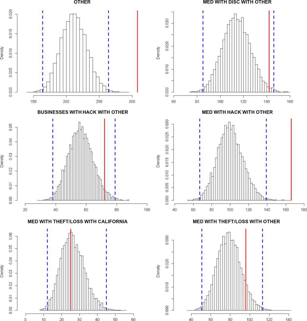
Figure 6 Distribution of the number of attacks predicted for 2016 with kernel 3 – in red the real number, in blue the 0.5% and 99.5% quantiles of the predicted distribution.

Figure 7 Distribution of the number of attacks predicted for 2017 with kernel 3 – in red the real number, in blue the 0.5% and 99.5% quantiles of the predicted distribution.
The model with kernel 3 (
 $\phi_{i,j}(t) = \alpha_{i,j}t\exp(-\beta_{i}t)$
) and no penalisation seems to be a good compromise in terms of predictions over the 2 years. This model appears to be the most reliable since it is also the one with the best likelihood.
$\phi_{i,j}(t) = \alpha_{i,j}t\exp(-\beta_{i}t)$
) and no penalisation seems to be a good compromise in terms of predictions over the 2 years. This model appears to be the most reliable since it is also the one with the best likelihood.
4.8 Predictions of the whole distribution of the number of attacks
We use the so-called thinning algorithm in order to simulate trajectories of Hawkes processes that are projections of a Hawkes process with past occurrences corresponding to the historical data. A detailed discussion on the thinning procedure for Hawkes processes is given in section 4 of Boumezoued (Reference Boumezoued2016). The histograms of predictions based on 10,000 simulations are depicted in Figures 6 and 7. These distributions could be used to determine a 99.5% percentile at a 1-year horizon in the context of a Solvency II internal model. The distributions seem to capture the main trends, excepted for two cases in 2016 and one case in 2017. Besides, we note a tendency for the model to underestimate the number of attacks, this is a feature of exponential kernels (that decrease very fast) that has already been pointed out by Hardiman et al. (Reference Hardiman, Bercot and Bouchaud2013) in a financial framework for modelling order books. The projection for group OTHER (group 1) is particularly bad, due to the lack of structure of this “catch-all” group.
Finally, the model with kernel 3 seems to capture a significant part of the dynamics, with a reasonable number of parameters. Due to the heterogeneity of the PRC data set, it is impossible to work globally on the whole data set, so we have split in different groups. The choice of the different groups, which should be more homogeneous as possible, is determinant in the prediction accuracy, as illustrated by the group OTHER that performs very badly. The advantage of our approach is that this joint mutually exciting model focuses on the whole joint distribution of numbers of attacks for each group, which is more accurate – but also more complex – than modelling marginal distributions, group per group. It thus allows to globally analyse the arrival of events, given some characteristics (type of the breached entity, type of breach and localisation). A counterpart of this joint model is that a lower fitting accuracy for a given group may propagate to other groups.
Besides, part of the discrepancy observed in Figures 6 and 7 is also due to the variation of the underlying exposure that inevitably impacts the number of attacks and the accuracy of the predictions. Although it is very difficult to assess the exposure for such a public data set, an insurer could enrich this joint mutually exciting model using its own data on exposure, which could then be integrated within the baseline intensity of the Hawkes processes (e.g. taking a baseline intensity proportional to the exposure).
5 Conclusion
This paper proposes a joint mutually exciting model to analyse and predict the arrivals of cyber events. It is achieved through multivariate Hawkes processes that capture the clustering and autocorrelation of times of cyber events, depending on some characteristics. The analysis is conducted on the public data set of PRC, on which different Hawkes kernels are calibrated. A kernel with a non-instantaneous excitation provides a better fit, compared to the standard exponential kernel. With such parsimonious parametric specifications, the model achieves reasonable forecasts which have been performed over a 1-year horizon. Besides, the methodology can be easily extended to other types of cyber data.
This is a first step towards using advanced stochastic processes for the computation of a solvency capital for cyber insurance or in the field of cyber risk covers pricing. An insurance pricing methodology requires the estimation of the frequency and severity of claims, while our methodology only focuses on the arrivals of cyber events.
First, our model should be completed with an exposure analysis in order to assess the pure frequency component of the risk. Unfortunately, since the PRC database is fed by various sources of information, the exposure – that is the number of entities exposed to risk within the PRC database – is difficult to handle. Therefore, it is almost impossible to know from such data which part of the variation along time of the reported claims is caused by an evolution of the risk, and which part is caused by an instability in the way the data are collected. On the contrary, an insurance portfolio has a better knowledge of its exposition. But even for an insurance company with a cyber portfolio, the frequency would be poorly estimated if only based on internal historical data, since the number of reported claims would be too small to perform an accurate estimation. That is why analysing public databases like PRC is important to improve the evaluation of the risk.
Second, for the severity component, the PRC data set does not report directly the financial loss resulting from a data breach event, but still a severity indication is given through the volume of data breached. A projected financial loss can be then estimated from the number of records, accordingly to previous approaches such as in Eling & Loperfido (Reference Eling and Loperfido2017) or more recently in Farkas et al. Let us note that Romanosky (Reference Romanosky2016) also studied the cost of data breaches using a private database gathering cyber events and associated losses. Again, an insurance company has a better knowledge of the effective losses of cyber events, but on a smaller data set. To conclude, combining insurance portfolio data with external information – including public databases like PRC – seems to be essential to improve the evaluation of the risk.
Acknowledgements
The authors acknowledge funding from the project Cyber Risk Insurance: actuarial modelling, Joint Research Initiative under the aegis of Risk Fundation, with partnership of AXA, AXA GRM, ENSAE and Sorbonne Université
Appendix A Repartition of Attacks by State (PRC)

Appendix B Computation of the Expectation of the Multivariate Non-Stationary Hawkes Process
In this section, we derive closed-form formulas for the expectation of the Hawkes process under the three kernel specifications as given in Equation (8). The proof relies on deriving the dynamics of the underlying age pyramid, as developed by Boumezoued (Reference Boumezoued2016) to compute the distribution of non-stationary Hawkes processes for general kernel in the univariate case; we extend here the scope of application of such techniques to the multivariate Hawkes model for the kernels considered.
In the population representation, events are interpreted as arrivals or births of individuals in a population, while the Hawkes process measures the evolution of the total population size over time. Considering, for example, the univariate case (
 $d=1$
), immigrants arrive (with age zero) in the population according to a Poisson process with rate
$d=1$
), immigrants arrive (with age zero) in the population according to a Poisson process with rate
 $\mu_t$
, then each immigrant with age a gives birth with rate
$\mu_t$
, then each immigrant with age a gives birth with rate
 $\phi(a)$
; more generally, every individual with age a in the population gives birth with rate
$\phi(a)$
; more generally, every individual with age a in the population gives birth with rate
 $\phi(a)$
.
$\phi(a)$
.
We introduce the random point measure
 $Z_{t}^{(i)}({{d}} a), i \in \{1,..,d\}$
defined as
$Z_{t}^{(i)}({{d}} a), i \in \{1,..,d\}$
defined as
 \begin{equation*}Z_{t}^{(i)}({{d}} a) = \int_{(0,t]}\delta _{t-s}({{d}} a){{d}} N^{(i)}_{s}=\sum_{n=1}^{N_{t}^{(i)}}\delta_{t-T_{n}^{(i)}}({{d}} a)\end{equation*}
This measure allows to keep track of all ages in the population and can be used to integrate a function f, to do this we use the notation
 \begin{equation*} \langle Z_{t}^{(i)}, f \rangle = \int_{\mathbb{R}^{+}}f(a)Z_{t}^{(i)}({{d}} a) = \int_{(0,t]}f(t-s){{d}} N_{s}^{(i)}\end{equation*}
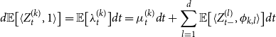
For instance, it allows us to represent the Hawkes process itself with
 $N_{t}^{(i)}=\langle Z_{t}^{(i)}, 1 \rangle$
or the intensity of the process
$N_{t}^{(i)}=\langle Z_{t}^{(i)}, 1 \rangle$
or the intensity of the process
 $(N_{t}^{(i)})_{t\geq0}$
with
$(N_{t}^{(i)})_{t\geq0}$
with
 \begin{equation*}\lambda^{(i)}_t = \mu^{(i)}_t +\sum_{j=1}^{d} \langle Z_{t-}^{(j)}, \phi_{i,j} \rangle\end{equation*}
The computation of the expectation will make use of the following result, see Lemma 1 in Boumezoued (Reference Boumezoued2016):
Proposition 3. For any differentiable function
 $f\,{:}\,\mathbb{R}_{+} \rightarrow \mathbb{R}$
with derivative f:
$f\,{:}\,\mathbb{R}_{+} \rightarrow \mathbb{R}$
with derivative f:
 \begin{equation*} \langle Z_{t}^{(j)}, f \rangle = f(0) \langle Z_{t}^{(j)}, 1 \rangle + \int_{0}^{t}\langle Z_{s}^{(j)}, f' \rangle{{d}} s, \,\mbox{ for any } j \in \{1,...,d\} \end{equation*}
In this dynamics, the first term refers to the pure jump part of arrivals of individuals with age 0, whereas the second term of transport type illustrates the aging phenomenon: all ages are translated along the time axis.
In the following, we provide closed-form calculations for the expectation of the multivariate Hawkes process for the three kernel specifications studied in this paper:
 \begin{align*}
&\text{Kernel 1: } \phi_{i,j}(t) =\alpha_{i,j}\exp(-\beta_{i}t)\nonumber\\[5pt]
&\text{Kernel 2: } \phi_{i,j}(t) =\alpha_{i,j}\exp(-\beta_{i,j}t)\\[5pt]
&\text{Kernel 3: } \phi_{i,j}(t) = \alpha_{i,j}t\exp(-\beta_{i}t)\nonumber\end{align*}
\begin{align*}
&\text{Kernel 1: } \phi_{i,j}(t) =\alpha_{i,j}\exp(-\beta_{i}t)\nonumber\\[5pt]
&\text{Kernel 2: } \phi_{i,j}(t) =\alpha_{i,j}\exp(-\beta_{i,j}t)\\[5pt]
&\text{Kernel 3: } \phi_{i,j}(t) = \alpha_{i,j}t\exp(-\beta_{i}t)\nonumber\end{align*}
Kernels 1 and 2 correspond to the exponential case and are studied in section B.1, whereas kernel 3 is tackled separately in section B.2.
B.1 Expectation with kernels 1 and 2 (exponential case)
Proposition 4. Let us consider a d-variate Hawkes process
 $(N_{t}^{(1)})_{t\geq0},...,(N_{t}^{(d)})_{t\geq0}$
with exponential kernel, and let us denote
$(N_{t}^{(1)})_{t\geq0},...,(N_{t}^{(d)})_{t\geq0}$
with exponential kernel, and let us denote
 $(\lambda_{t}^{(i)})_{t\geq0}$
the intensity process of the process
$(\lambda_{t}^{(i)})_{t\geq0}$
the intensity process of the process
 $(N_{t}^{(i)})_{t\geq0}$
:
$(N_{t}^{(i)})_{t\geq0}$
:
 \begin{equation*}\lambda^{(i)}_t =\mu^{(i)}_t+\sum_{j=1}^{d}\int_{[0,t[}\phi_{i,j}(t-s){{d}} N^{(j)}_{s}=\mu^{(i)}_t+\sum_{j=1}^{d}\sum_{T^{(j)}_{n}<t}\alpha_{i,j}\exp\left(-\beta_{i,j}\left(t-T^{(j)}_{n}\right)\right)\end{equation*}
with
 $\mu^{(i)}\,:\,\mathbb{R}^+ \longrightarrow \mathbb{R}^+, \, \, (\alpha_{i,j})_{1\leq i,j\leq d} \in \mathbb{R}_{+}^{d\times d}, \, \,(\beta_{i,j})_{1\leq i,j\leq d} \in \mathbb{R}_{+}^{d\times d}.$
We define the vector
 $X_t$
and its expectation:
$X_t$
and its expectation:
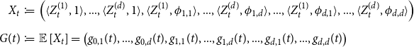 \begin{eqnarray*}X_{t}&\coloneqq &\Big(\langle Z_{t}^{(1)}, 1 \rangle,...,\langle Z_{t}^{(d)}, 1 \rangle,\langle Z_{t}^{(1)}, \phi_{1,1} \rangle,...,\langle Z_{t}^{(d)}, \phi_{1,d} \rangle,...,\langle Z_{t}^{(1)}, \phi_{d,1} \rangle,...,\langle Z_{t}^{(d)}, \phi_{d,d} \rangle \Big)\\[5pt]
G(t) &\coloneqq & {\mathbb{E}} \left[X_t \right]=\big(g_{0,1}(t),...,g_{0,d}(t),g_{1,1}(t),...,g_{1,d}(t),...,g_{d,1}(t),...,g_{d,d}(t)\big)\end{eqnarray*}
\begin{eqnarray*}X_{t}&\coloneqq &\Big(\langle Z_{t}^{(1)}, 1 \rangle,...,\langle Z_{t}^{(d)}, 1 \rangle,\langle Z_{t}^{(1)}, \phi_{1,1} \rangle,...,\langle Z_{t}^{(d)}, \phi_{1,d} \rangle,...,\langle Z_{t}^{(1)}, \phi_{d,1} \rangle,...,\langle Z_{t}^{(d)}, \phi_{d,d} \rangle \Big)\\[5pt]
G(t) &\coloneqq & {\mathbb{E}} \left[X_t \right]=\big(g_{0,1}(t),...,g_{0,d}(t),g_{1,1}(t),...,g_{1,d}(t),...,g_{d,1}(t),...,g_{d,d}(t)\big)\end{eqnarray*}
Then the dynamics of
 $X_t$
is Markovian and G(t) can be expressed, for
$X_t$
is Markovian and G(t) can be expressed, for
 $t_0<t$
, as:
$t_0<t$
, as:
 \begin{equation*} G(t) = G(t_{0})\exp(A(t-t_{0}))+\int_{t_{0}}^{t}\exp(A(t-s))B(s) {{d}} s\end{equation*}
B(t) is a vector with size
 $d(d+1)$
defined below:
$d(d+1)$
defined below:
-
• for each
$1\leq i\leq d$
,
$[B(t)]_{i}=\mu^{(i)}_t$
; -
• for each
$d+1\leq i\leq d^2+d$
, such that
$i=ad+b$
with integers a and b such that
$1\leq a \leq d$
and
$1 \leq b \leq d$
,
$[B(t)]_{i}=\alpha_{a,b}\mu^{(b)}_t$
.


A is a matrix with size
 $d(d+1)\times d(d+1)$
defined as follows:
$d(d+1)\times d(d+1)$
defined as follows:
-
• for
$1\leq m\leq d$
:
$[A]_{m,n}=1$
with
$md+1\leq n \leq md+d$
; -
• for
$d+1\leq m\leq d^2+d$
such that
$m=ad+b,$
with integers a and b such that
$1\leq a \leq d$
and
$1 \leq b \leq d$
;
-
– If
$a \neq b$
,
-
*
$[A]_{m,m}=-\beta_{a,b}$
-
*
$[A]_{m,n}=\alpha_{a,b}$
for any
$bd+1\leq n \leq bd+d$
-
-
– If
$a = b$
,
-
*
$[A]_{m,m}=\alpha_{a,a}-\beta_{a,a}$
-
*
$[A]_{m,n}=\alpha_{a,a}$
for any
$bd+1\leq n \leq bd+d$
and
$n\neq m$
-
-


Note that non-specified components are zero.
Proof of Proposition
4. Let us prove in a first step that the dynamics of
 $(X_t)_{t\geq0}$
is Markovian. In particular, let us determine the dynamics of
$(X_t)_{t\geq0}$
is Markovian. In particular, let us determine the dynamics of
 $\langle Z_{t}^{(j)}, \phi_{i,j} \rangle $
with
$\langle Z_{t}^{(j)}, \phi_{i,j} \rangle $
with
 $1\leq i,j \leq d$
, keeping in mind that
$1\leq i,j \leq d$
, keeping in mind that
 $\phi_{i,j}$
represents the influence of
$\phi_{i,j}$
represents the influence of
 $(N_{t}^{(j)})_{t\geq0}$
on the intensity of
$(N_{t}^{(j)})_{t\geq0}$
on the intensity of
 $(N_{t}^{(i)})_{t\geq0}$
; by using Proposition 3,
$(N_{t}^{(i)})_{t\geq0}$
; by using Proposition 3,
 \begin{equation*} \begin{split} \langle Z_{t}^{(j)}, \phi_{i,j} \rangle &= \alpha_{i,j}N_{t}^{(j)}+\int_{0}^{t}\langle Z_{s}^{(j)}, \phi'_{i,j} \rangle {{d}} s \\[6pt]
&= \alpha_{i,j}N_{t}^{(j)}-\beta_{i,j}\int_{0}^{t}\langle Z_{s}^{(j)}, \phi_{i,j} \rangle {{d}} s \\ \end{split}\end{equation*}
\begin{equation*} \begin{split} \langle Z_{t}^{(j)}, \phi_{i,j} \rangle &= \alpha_{i,j}N_{t}^{(j)}+\int_{0}^{t}\langle Z_{s}^{(j)}, \phi'_{i,j} \rangle {{d}} s \\[6pt]
&= \alpha_{i,j}N_{t}^{(j)}-\beta_{i,j}\int_{0}^{t}\langle Z_{s}^{(j)}, \phi_{i,j} \rangle {{d}} s \\ \end{split}\end{equation*}
By differentiation, we obtain
 \begin{equation} {{d}} \langle Z_{t}^{(j)}, \phi_{i,j} \rangle = \alpha_{i,j}{{d}} N_{t}^{(j)}-\beta_{i,j}\langle Z_{t}^{(j)}, \phi_{i,j} \rangle {{d}} t \end{equation}
Therefore, the dynamics of
 $(X_{t})_{t\geq0}$
is Markovian.
$(X_{t})_{t\geq0}$
is Markovian.
Let us find in a second step the form of G. Let us define
 $g_{i,j}(t) = \mathbb{E}\big[\langle Z_{t}^{(j)}, \phi_{i,j} \rangle \big]$
, and let us take the expectation in (B.2) using the fact that
$g_{i,j}(t) = \mathbb{E}\big[\langle Z_{t}^{(j)}, \phi_{i,j} \rangle \big]$
, and let us take the expectation in (B.2) using the fact that
 $\mathbb{E}[{{d}} N_{t}^{(j)}]=\mathbb{E}[\lambda^{(j)}_t]{{d}} t$
:
$\mathbb{E}[{{d}} N_{t}^{(j)}]=\mathbb{E}[\lambda^{(j)}_t]{{d}} t$
:
 \begin{equation*}\begin{split} {{d}} \mathbb{E}\big[\langle Z_{t}^{(j)}, \phi_{i,j} \rangle \big]&= \alpha_{i,j}\mathbb{E}\big[\lambda^{(j)}_t\big] {{d}} t-\beta_{i,j}\mathbb{E}\big[\langle Z_{t}^{(j)}, \phi_{i,j} \rangle\big] {{d}} t \\ &=\alpha_{i,j}\mu^{(j)}_t {{d}} t + \alpha_{i,j}\sum_{k=1}^{d} \mathbb{E}\Big[\langle Z_{t-}^{(k)}, \phi_{j,k} \rangle \Big]{{d}} t - \beta_{i,j}g_{i,j}(t){{d}} t\end{split}\end{equation*}
By using the fact that Lebesgue measure charges no point, we obtain
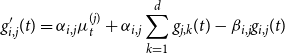 \begin{equation*} \begin{split} g_{i,j}^{\prime}(t) &=\alpha_{i,j}\mu^{(j)}_t +\alpha_{i,j} \sum_{k=1}^{d}g_{j,k}(t) - \beta_{i,j}g_{i,j}(t)\\ \end{split}\end{equation*}
Now let us study the expectation of
 $N_{t}^{(k)}=\langle Z_{t}^{(k)}, 1 \rangle $
for
$N_{t}^{(k)}=\langle Z_{t}^{(k)}, 1 \rangle $
for
 $1\leq k \leq d$
:
$1\leq k \leq d$
:
 \begin{equation*} {{d}} \mathbb{E}\big[\langle Z_{t}^{(k)}, 1 \rangle \big]= \mathbb{E}\big[ \lambda_{t}^{(k)}\big]{{d}} t = \mu^{(k)}_t {{d}} t+\sum_{l=1}^{d} \mathbb{E}\big[ \langle Z_{t-}^{(l)}, \phi_{k,l} \rangle\big]{{d}} t\end{equation*}
Let us set
 $g_{0,k}(t)=\mathbb{E}\big[\langle Z_{t}^{(k)}, 1 \rangle \big]$
, then
$g_{0,k}(t)=\mathbb{E}\big[\langle Z_{t}^{(k)}, 1 \rangle \big]$
, then
 \begin{equation*}g^{\prime}_{0,k}(t)=\mu^{(k)}_t+\sum_{l=1}^{d}g_{k,l}(t)\end{equation*}
Therefore, the system of differential equations can be conveniently rewritten as
 \begin{equation*}G'(t)=AG(t)+B(t)\end{equation*}
where A and B(t) are specified in Proposition 4; this finally proves that G is of the form:
 \begin{equation*} G(t) = G(t_{0})\exp(A(t-t_{0}))+\int_{t_{0}}^{t}\exp(A(t-s))B(s) {{d}} s\end{equation*}
Remark 4. The proof to obtain expectations conditional on information up to any time is similar.
B.2 Expectation with kernel 3
The next proposition provides the computation for a d-variate Hawkes process with kernel
 $\phi_{i,j}(a)=\alpha_{i,j} a\exp(-\beta_{i,j}a)$
, which is little bit more general than kernel 3 that corresponds to
$\phi_{i,j}(a)=\alpha_{i,j} a\exp(-\beta_{i,j}a)$
, which is little bit more general than kernel 3 that corresponds to
 $\beta_{i,j}=\beta_i$
for all j.
$\beta_{i,j}=\beta_i$
for all j.
Proposition 5 Let us consider a d-variate Hawkes process with kernel
 $\phi_{i,j}(a)=\alpha_{i,j} a\exp(-\beta_{i,j}a)$
. Let us still denote by
$\phi_{i,j}(a)=\alpha_{i,j} a\exp(-\beta_{i,j}a)$
. Let us still denote by
 $(\lambda_{t}^{(i)})_{t\geq0}$
the intensity process of the process
$(\lambda_{t}^{(i)})_{t\geq0}$
the intensity process of the process
 $(N_{t}^{(i)})_{t\geq0}, i \in \{1,...,d\}$
:
$(N_{t}^{(i)})_{t\geq0}, i \in \{1,...,d\}$
:
 \begin{equation*}\lambda^{(i)}_t =\mu^{(i)}_t+\sum_{j=1}^{d}\int_{[0,t[}\phi_{i,j}(t-s){{d}} N^{(j)}_{s}=\mu^{(i)}_t+\sum_{j=1}^{d}\sum_{T^{(j)}_{n}<t}\alpha_{i,j}\left(t-T^{(j)}_{n}\right)\exp\left(-\beta_{i,j}\left(t-T^{(j)}_{n}\right)\right)\end{equation*}
with
 $\mu^{(i)}\,{:}\,\mathbb{R}^+ \longrightarrow \mathbb{R}^+, \, \, (\alpha_{i,j})_{1\leq i,j\leq d} \in \mathbb{R}_{+}^{d\times d}, \, \,(\beta_{i,j})_{1\leq i,j\leq d} \in \mathbb{R}_{+}^{d\times d}.$
Now let us consider the following vector
 $Y_t$
and its expectation
$Y_t$
and its expectation
 $H_t$
:
$H_t$
:
 \begin{eqnarray*}Y_{t}&\coloneqq &\left(\left(\langle Z_{t}^{(i)}, 1 \rangle\right)_{1\leq i\leq d},\left(\langle Z_{t}^{(j)}, \phi_{i,j}\right)_{1\leq i,j\leq d}, \left(\langle Z_{t}^{(j)}, \phi_{i,j}^{(e)}\right)_{1\leq i,j\leq d} \right) \\H(t) &: =& {\mathbb{E}} \left[ Y_{t}\right]\end{eqnarray*}
with same ordering as for X in Proposition 4, and using the notation
 $\phi_{i,j}^{(e)}(a)=\alpha_{i,j}\exp(-\beta_{i,j}a)$
for the exponential kernel. Then, the dynamics of
$\phi_{i,j}^{(e)}(a)=\alpha_{i,j}\exp(-\beta_{i,j}a)$
for the exponential kernel. Then, the dynamics of
 $Y_t$
is Markovian and, in particular H(t), can be expressed for
$Y_t$
is Markovian and, in particular H(t), can be expressed for
 $t>t_0$
as
$t>t_0$
as
 \begin{equation*}H(t) = H(t_{0})\exp(C(t-t_{0}))+\int_{t_{0}}^{t}\exp(C(t-s))D(s) {{d}} s\end{equation*}
D(t) is a vector with size
 $d(2d+1)$
defined below:
$d(2d+1)$
defined below:
-
• for each
$1\leq i\leq d$
,
$[D(t)]_{i}=\mu^{(i)}_t$
; -
• for each
$d^2+d+1\leq i\leq 2d^2+d$
such that
$i=d^2+ad+b$
with integers a and b such that
$1\leq a \leq d$
and
$1 \leq b \leq d$
,
$[D(t)]_{i}=\alpha_{a,b} \mu^{(b)}_t$
.


C is a matrix with size
 $d(2d+1)\times d(2d+1)$
defined as follows:
$d(2d+1)\times d(2d+1)$
defined as follows:
-
• for
$1\leq m\leq d$
:
$[C]_{m,n}=1$
with
$md+1\leq n \leq md+d;$
-
• for
$d+1\leq m\leq d^2+d$
such that
$m=ad+b,$
with integers a and b such that
$1\leq a \leq d$
and
$1 \leq b \leq d$
:
-
–
$[C]_{m,m}=-\beta_{a,b}$
-
–
$[C]_{m,m+d^2}=1$
;
-
-
• for
$d^2+d+1\leq m\leq 2d^2+d$
such that
$m=ad+b,$
with integers a and b such that
$1\leq a \leq d$
and
$1 \leq b \leq d$
:
-
–
$[C]_{m,m}=-\beta_{a,b}$
-
–
$[C]_{m,n}=\alpha_{a,b}$
with
$bd+1\leq n \leq bd+d$
.
-


Note that non-specified components are zero.
Proof of Proposition
5. Let us first notice that
 $\phi_{i,j}^{\prime}(a)=\phi_{i,j}^{(e)}(a)-\beta_{i,j}\phi_{i,j}(a)$
where we redefine the exponential kernel as
$\phi_{i,j}^{\prime}(a)=\phi_{i,j}^{(e)}(a)-\beta_{i,j}\phi_{i,j}(a)$
where we redefine the exponential kernel as
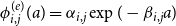 \begin{equation*}\phi_{i,j}^{(e)}(a)=\alpha_{i,j}\exp(-\beta_{i,j}a)\end{equation*}
The dynamics of
 $(\langle Z_{t}^{(i)}, 1 \rangle)_{1 \leq i \leq d}$
is the same as in the proof for the exponential case, and we get
$(\langle Z_{t}^{(i)}, 1 \rangle)_{1 \leq i \leq d}$
is the same as in the proof for the exponential case, and we get
 \begin{equation} g^{\prime}_{0,k}(t)=\mu^{(k)}_t+\sum_{l=1}^{d}g_{k,l}(t)\end{equation}
where we set
 $g_{0,k}(t)=\mathbb{E}\big[\langle Z_{t}^{(k)}, 1 \rangle \big]$
and
$g_{0,k}(t)=\mathbb{E}\big[\langle Z_{t}^{(k)}, 1 \rangle \big]$
and
 $g_{i,j}(t) = \mathbb{E}\big[\langle Z_{t}^{(j)}, \phi_{i,j} \rangle \big].$
Let us now study the dynamics of
 $\langle Z_{t}^{(j)}, \phi_{i,j} \rangle$
for
$\langle Z_{t}^{(j)}, \phi_{i,j} \rangle$
for
 $1\leq i,j \leq d$
:
$1\leq i,j \leq d$
:
 \begin{equation*} \begin{split} {{d}} \langle Z_{t}^{(j)}, \phi_{i,j} \rangle &= \phi_{i,j}(0){{d}} N_{t}^{(j)}+\langle Z_{t}^{(j)}, \phi'_{i,j} \rangle {{d}} t \\[5pt]
&= \langle Z_{t}^{(j)}, \phi_{i,j}^{(e)} \rangle {{d}} t -\beta_{i,j}\langle Z_{t}^{(j)}, \phi_{i,j} \rangle {{d}} t \end{split}\end{equation*}
\begin{equation*} \begin{split} {{d}} \langle Z_{t}^{(j)}, \phi_{i,j} \rangle &= \phi_{i,j}(0){{d}} N_{t}^{(j)}+\langle Z_{t}^{(j)}, \phi'_{i,j} \rangle {{d}} t \\[5pt]
&= \langle Z_{t}^{(j)}, \phi_{i,j}^{(e)} \rangle {{d}} t -\beta_{i,j}\langle Z_{t}^{(j)}, \phi_{i,j} \rangle {{d}} t \end{split}\end{equation*}
By taking expectation, we then get
 \begin{equation} g_{i,j}^{\prime}(t)=g_{i,j}^{(e)}(t)-\beta_{i,j} g_{i,j}(t)\end{equation}
where we set
 $g_{i,j}^{(e)}(t) = \mathbb{E}\big[\langle Z_{t}^{(j)}, \phi_{i,j}^{(e)} \rangle \big].$
Finally, let us study the dynamics of
$g_{i,j}^{(e)}(t) = \mathbb{E}\big[\langle Z_{t}^{(j)}, \phi_{i,j}^{(e)} \rangle \big].$
Finally, let us study the dynamics of
 $\langle Z_{t}^{(j)}, \phi_{i,j}^{(e)} \rangle$
:
$\langle Z_{t}^{(j)}, \phi_{i,j}^{(e)} \rangle$
:
 \begin{equation*} {{d}} \langle Z_{t}^{(j)}, \phi_{i,j}^{(e)} \rangle = \alpha_{i,j}{{d}} N_{t}^{(j)}-\beta_{i,j}\langle Z_{t}^{(j)}, \phi_{i,j}^{(e)} \rangle {{d}} t \end{equation*}
By taking expectation, we get
 \begin{equation*}\begin{split} {{d}} \mathbb{E}\left[\langle Z_{t}^{(j)}, \phi_{i,j}^{(e)} \rangle \right]&= \alpha_{i,j}\mathbb{E}\left[\lambda^{(j)}_t\right] {{d}} t-\beta_{i,j}\mathbb{E}\left[\langle Z_{t}^{(j)}, \phi_{i,j}^{(e)} \rangle\right] {{d}} t \\ &=\alpha_{i,j}\mu^{(j)}_t {{d}} t + \alpha_{i,j}\sum_{k=1}^{d} \mathbb{E}\Big[\langle Z_{t-}^{(k)}, \phi_{j,k} \rangle \Big]{{d}} t - \beta_{i,j}g_{i,j}^{(e)}(t){{d}} t\\\end{split}\end{equation*}
leading to the differential equation:
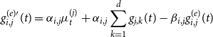 \begin{equation} g_{i,j}^{(e)\prime}(t)= \alpha_{i,j}\mu^{(j)}_t + \alpha_{i,j}\sum_{k=1}^{d} g_{j,k}(t) - \beta_{i,j}g_{i,j}^{(e)}(t) \end{equation}
From Equations (B.3), (B.4) and (B.5), the ordinary differential equation for
 $H(t) = {\mathbb{E}} \left[ Y_{t}\right]$
can therefore be rewritten as
$H(t) = {\mathbb{E}} \left[ Y_{t}\right]$
can therefore be rewritten as
 \begin{equation*}H'(t)=CH(t)+D(t)\end{equation*}
where C and D(t) are specified in Proposition 2, which finally proves that H can be computed as
 \begin{equation*} H(t) = H(t_{0})\exp(C(t-t_{0}))+\int_{t_{0}}^{t}\exp(C(t-s))D(s) {{d}} s\end{equation*}


