


Impact Statement
Climate change will affect wind and, therefore, wind power; climate models can help to gain insights into future power generation. Using Gaussian processes, we project wind power output given wind speeds from a global climate model. We show that turbine locations are essential for accurate multi-decadal power projections. We show that for the more likely climate scenarios, only minor changes in wind power generation are expected—indicating that wind energy can continue to be a reliable energy source in the upcoming years.
1. Introduction
To mitigate climate change, wind energy will play an essential role in the future power supply (Barthelmie and Pryor, Reference Barthelmie and Pryor2021). Efficient power planning should, therefore, account for natural wind variability as well as climate change by incorporating climate projections into multi-decadal predictions (e.g., Miao et al., Reference Miao, Xu, Huang and Yang2023. However, these climate projections have two main shortcomings: Their output resolutions are coarse due to the high (computational) complexity of climate models and are uncertain as they account for, among other things, unpredictable human behavior.
To overcome the issue of coarse spatial resolution (usually
 $ \ge 100 $
km) of general circulation models (GCMs), so-called downscaling techniques have been developed (e.g., Sun et al., Reference Sun, Deng, Ren, Liu, Deng and Jin2024). Downscaling, including statistical and machine learning methods (e.g., Langguth et al., Reference Langguth, Harder, Schicker, Patnala, Lehner, Mayer and Dabernig2024) and dynamical downscaling, can increase the spatial but also the temporal resolution of GCMs. For multi-decadal wind power predictions, where the primary goal is an accurate cumulative power prediction, Effenberger et al. (Reference Effenberger, Ludwig and White2023) have shown that a temporal resolution of 6 hours is generally sufficient. An analogous observation has not yet been made for spatial resolutions; a high spatial resolution is often beneficial (e.g., Tamoffo et al., Reference Tamoffo, Dosio, Vondou and Sonkoué2020) and can resolve more physical processes and weather phenomena (Letson et al., Reference Letson, Shepherd, Barthelmie and Pryor2020) but requires careful selection (Pryor et al., Reference Pryor, Barthelmie, Bukovsky, Leung and Sakaguchi2020). For CMIP6 (Eyring et al., Reference Eyring, Bony, Meehl, Senior, Stevens, Stouffer and Taylor2016), the latest version of globally organized GCMs, no high-resolution regional model runs are available yet, in contrast to its predecessor CMIP5 (compare e.g., Jacob et al., Reference Jacob, Petersen, Eggert, Alias, Christensen, Bouwer, Braun, Colette, Déqué and Georgievski2014). To overcome this issue, Bartók et al. (Reference Bartók, Tobin, Vautard, Vrac, Jin, Levavasseur, Denvil, Dubus, Parey and Michelangeli2019) have developed a climate projection dataset tailored for the European energy sector based on CMIP5. Previous research, however, revealed that CMIP6 and CMIP5 show differences in future wind resource projections for Europe (Carvalho et al., Reference Carvalho, Rocha, Costoya, DeCastro and Gómez-Gesteira2021), with CMIP6 showing better capability in simulating past surface wind speeds across the entire Northern Hemisphere (Miao et al., Reference Miao, Xu, Huang and Yang2023). However, there is an important difference between historical and future climate model data, as climate models do not only predict one future scenario of the atmosphere. A critical point of climate models is their ability to integrate radiative forcing and represent different future scenarios. In this context, Jung and Schindler (Reference Jung and Schindler2022) show that the unlikely worst-case climate model scenario SSP5–8.5 (Hausfather and Peters, Reference Hausfather and Peters2020) is over-represented in current research. Therefore, while the plausibility of different scenarios is unclear (e.g., Pielke Jr et al., Reference Pielke, Burgess and Ritchie2022), there is a need for projecting realistic scenarios of CMIP6 for multi-decadal power prediction.
$ \ge 100 $
km) of general circulation models (GCMs), so-called downscaling techniques have been developed (e.g., Sun et al., Reference Sun, Deng, Ren, Liu, Deng and Jin2024). Downscaling, including statistical and machine learning methods (e.g., Langguth et al., Reference Langguth, Harder, Schicker, Patnala, Lehner, Mayer and Dabernig2024) and dynamical downscaling, can increase the spatial but also the temporal resolution of GCMs. For multi-decadal wind power predictions, where the primary goal is an accurate cumulative power prediction, Effenberger et al. (Reference Effenberger, Ludwig and White2023) have shown that a temporal resolution of 6 hours is generally sufficient. An analogous observation has not yet been made for spatial resolutions; a high spatial resolution is often beneficial (e.g., Tamoffo et al., Reference Tamoffo, Dosio, Vondou and Sonkoué2020) and can resolve more physical processes and weather phenomena (Letson et al., Reference Letson, Shepherd, Barthelmie and Pryor2020) but requires careful selection (Pryor et al., Reference Pryor, Barthelmie, Bukovsky, Leung and Sakaguchi2020). For CMIP6 (Eyring et al., Reference Eyring, Bony, Meehl, Senior, Stevens, Stouffer and Taylor2016), the latest version of globally organized GCMs, no high-resolution regional model runs are available yet, in contrast to its predecessor CMIP5 (compare e.g., Jacob et al., Reference Jacob, Petersen, Eggert, Alias, Christensen, Bouwer, Braun, Colette, Déqué and Georgievski2014). To overcome this issue, Bartók et al. (Reference Bartók, Tobin, Vautard, Vrac, Jin, Levavasseur, Denvil, Dubus, Parey and Michelangeli2019) have developed a climate projection dataset tailored for the European energy sector based on CMIP5. Previous research, however, revealed that CMIP6 and CMIP5 show differences in future wind resource projections for Europe (Carvalho et al., Reference Carvalho, Rocha, Costoya, DeCastro and Gómez-Gesteira2021), with CMIP6 showing better capability in simulating past surface wind speeds across the entire Northern Hemisphere (Miao et al., Reference Miao, Xu, Huang and Yang2023). However, there is an important difference between historical and future climate model data, as climate models do not only predict one future scenario of the atmosphere. A critical point of climate models is their ability to integrate radiative forcing and represent different future scenarios. In this context, Jung and Schindler (Reference Jung and Schindler2022) show that the unlikely worst-case climate model scenario SSP5–8.5 (Hausfather and Peters, Reference Hausfather and Peters2020) is over-represented in current research. Therefore, while the plausibility of different scenarios is unclear (e.g., Pielke Jr et al., Reference Pielke, Burgess and Ritchie2022), there is a need for projecting realistic scenarios of CMIP6 for multi-decadal power prediction.
Several studies investigate potential changes in wind power resources due to climate change. The studies primarily differ in the data used and the study region considered. We refer to Jung and Schindler (Reference Jung and Schindler2022) for an overview of recent studies on wind resource projections under climate change and summarize some main points and more recent work here. Gernaat et al. (Reference Gernaat, de Boer, Daioglou, Yalew, Müller and van Vuuren2021) investigate data from CMIP5 and find that changes in wind energy are uncertain with complex patterns across climate models; Barkanov et al. (Reference Barkanov, Penalba, Martinez, Martinez-Perurena, Zarketa-Astigarraga and Iglesias2024) investigate raw CMIP6 data and reveal changes in European offshore renewable energy resources. Martinez and Iglesias (Reference Martinez and Iglesias2024) find a significant decline in wind resources by 2100 in CMIP6, particularly evident in the mid-latitudes of the Northern Hemisphere; for Germany, they find negligible changes in wind power generation in the long-term future (2091–2100) under the high emission climate change scenario SSP5–8.5. Investigating CORDEX climate model data (compare Jacob et al., Reference Jacob, Petersen, Eggert, Alias, Christensen, Bouwer, Braun, Colette, Déqué and Georgievski2014) for 2025–2049, Sander et al. (Reference Sander, Jung and Schindler2021) support this claim and find that climate change will affect wind energy in Germany only marginally. Several studies investigate regions out of the scope of this study (e.g., Nabipour et al., Reference Nabipour, Mosavi, Hajnal, Nadai, Shamshirband and Chau2020; Martinez and Iglesias, Reference Martinez and Iglesias2022; He et al., Reference He, Chan, Li and Tong2023); all reveal similar results in terms of the complexity of spatial and temporal patterns.
As most of the renewable power data is confidential, using wind speeds (Jung and Schindler, Reference Jung and Schindler2020) or wind speeds cubed (Miao et al., Reference Miao, Xu, Huang and Yang2023) as a proxy for wind power is common. Most of the reviewed work considers gridded climate data only; however, some research also incorporates turbine locations for more realistic power predictions (e.g., Tobin et al., Reference Tobin, Jerez, Vautard, Thais, Van Meijgaard, Prein, Déqué, Kotlarski, Maule and Nikulin2016; Jung and Schindler, Reference Jung and Schindler2020). In this work, we further expand the framework of location awareness by predicting turbine location-aware multi-decadal wind power and validating these predictions with actual wind power generation.
Using CMIP6 data directly, we account for the latest climate model updates. The framework of Gaussian processes (GPs) allows us to additionally include turbine locations in our power projections, and we show that these are similar to the ground truth aggregated power generation. GPs have proven useful in recent wind power assessment studies e.g., by Moradian et al. (Reference Moradian, Gharbia, Nezhad and Olbert2024) or Esnaola et al. (Reference Esnaola, Ulazia, Sáenz and Ibarra-Berastegi2024) as well as downscaling climate variables (e.g., Chau et al., Reference Chau, Bouabid and Sejdinovic2021; Kupilik et al., Reference Kupilik, Witmer and Grill2024). In most cases, downscaling refers to increasing the resolution of gridded data (compare Sun et al., Reference Sun, Deng, Ren, Liu, Deng and Jin2024). One main advantage of GPs compared to other statistical downscaling approaches is that they do not rely on a grid. This makes them a natural choice for turbine location-specific downscaling. Additionally, their probabilistic framework can be useful in climate modeling where projections are usually associated with high uncertainty (Lehner et al., Reference Lehner, Deser, Maher, Marotzke, Fischer, Brunner, Knutti and Hawkins2020).
In this work, we present a new approach for validating multi-decadal wind power predictions and provide turbine location-aware predictions for Germany up to 2050. We describe our approach in Section 2, our results in Section 3, and discuss and conclude in Sectios 4 and 5.
2. Methods
Our general approach includes 1) estimating wind speeds at turbine locations, 2) extrapolating wind speeds to hub height, and 3) predicting the corresponding power output. We compare the wind speeds at turbine locations to predictions that do not consider actual turbine placement but are based on gridded weather or climate datasets. We perform the same steps on these datasets, but 1) use the wind speeds at grid points, 2) extrapolate wind speeds to the average hub height, and 3) compute the power output using the most common turbine across the dataset.
2.1. Data
For our evaluation, we consider the gridded reanalysis dataset ERA5 (Hersbach et al., Reference Hersbach, Bell, Berrisford, Hirahara, Horányi, Muñoz-Sabater, Nicolas, Peubey, Radu and Schepers2020) and the gridded climate dataset MPI-ESM1.2-HR (Müller et al., Reference Müller, Jungclaus, Mauritsen, Baehr, Matthias Bittner, Bunzel, Esch, Ghosh and Haak2018) from CMIP6. Furthermore, we compare our predictions generated using these weather and climate datasets to aggregated transmission level power generation. The power data was collected from individual transmission system operators (TSOs) across Germany (OPSD, 2024) and data provided by the German federal agency “Bundesnetzagentur” through the SMARD database (Bundesnetzagentur, 2024). We use a turbine dataset provided by Manske and Schmiedt (Reference Manske and Schmiedt2023) to access the turbine locations and other static turbine data. For the gridded data that covers Germany, we set the boundaries in ERA5 to longitudes
 $ \in \left[5{}^{\circ},15{}^{\circ}\right] $
and latitudes
$ \in \left[5{}^{\circ},15{}^{\circ}\right] $
and latitudes
 $ \in \left[47{}^{\circ},56{}^{\circ}\right] $
. In the CMIP6 model runs, the boundaries of the box considered are longitudes
$ \in \left[47{}^{\circ},56{}^{\circ}\right] $
. In the CMIP6 model runs, the boundaries of the box considered are longitudes
 $ \in \left[5.63{}^{\circ},\mathrm{15.0}{}^{\circ}\right] $
and latitudes
$ \in \left[5.63{}^{\circ},\mathrm{15.0}{}^{\circ}\right] $
and latitudes
 $ \in \left[47.22{}^{\circ},\mathrm{55.63}{}^{\circ}\right] $
and use all climate scenarios available for MPI-ESM1.2-HR, namely SSP1–2.6, SSP2–4.5, SSP3–7.0, SSP5–8.5. The recent work of Morelli (Reference Morelli2024) motivates our model selection, which finds that the MPI-ESM1.2-HR model represents the wind speed distribution across Germany particularly faithfully. As suggested by Effenberger et al. (Reference Effenberger, Ludwig and White2023), we use 6-hourly wind speed data. For an overview of the data used, see Figure 1.
$ \in \left[47.22{}^{\circ},\mathrm{55.63}{}^{\circ}\right] $
and use all climate scenarios available for MPI-ESM1.2-HR, namely SSP1–2.6, SSP2–4.5, SSP3–7.0, SSP5–8.5. The recent work of Morelli (Reference Morelli2024) motivates our model selection, which finds that the MPI-ESM1.2-HR model represents the wind speed distribution across Germany particularly faithfully. As suggested by Effenberger et al. (Reference Effenberger, Ludwig and White2023), we use 6-hourly wind speed data. For an overview of the data used, see Figure 1.

Figure 1. We use weather (ERA5), climate (CMIP6 historical and SSPs), and power data (TSO and SMARD) between 2011 and 2023. Due to limited data availability, not all datasets are temporally aligned.
2.2. Estimate wind speeds at turbine locations
Using the gridded climate and weather datasets described in the previous section, we compute wind speeds at turbine locations using Gaussian processes (GPs), see Figure 2 for an example. A GP is a collection of random variables where any finite subset follows a multivariate normal distribution. A GP is defined by a mean function
 $ \mu \left(\cdot \right) $
and a covariance function
$ \mu \left(\cdot \right) $
and a covariance function
 $ k\left(\cdot, \cdot \right) $
that is a positive definite kernel, see Equation (2.2). We consider the case where the output of the climate models is noisy, that is the underlying function
$ k\left(\cdot, \cdot \right) $
that is a positive definite kernel, see Equation (2.2). We consider the case where the output of the climate models is noisy, that is the underlying function
 $ f(x) $
is corrupted by Gaussian noise and therefore
$ f(x) $
is corrupted by Gaussian noise and therefore
 $$ y=f(x)+\unicode{x025B}, \hskip1.12em \mathrm{where}\hskip0.4em \unicode{x025B} \sim \mathcal{N}\left(0,{\sigma}^2\right). $$

Figure 2. Turbine locations and the corresponding wind speeds on January 1st 2011 (left) and 2023 (right), respectively. In Germany, there are more turbines in the North than in the South, and wind speeds are usually higher in the North.
We compute
 $ {\sigma}^2 $
as the variance over time of the two model runs available on the ESGF website (ESGF, 2024). To keep extreme values of the individual model runs, we do not use the mean of the model runs as input, but only the first model run r1i1p1f1. In GP regression, we put a GP prior on
$ {\sigma}^2 $
as the variance over time of the two model runs available on the ESGF website (ESGF, 2024). To keep extreme values of the individual model runs, we do not use the mean of the model runs as input, but only the first model run r1i1p1f1. In GP regression, we put a GP prior on
 $ f $
and compute the posterior given data
$ f $
and compute the posterior given data
 $ D={\left({x}_i,{y}_i\right)}_{i=1}^n=: \left\{\mathbf{X},y\right\} $
. The posterior is also a GP and can be computed analytically. For further details, we refer to Murphy (Reference Murphy2022). In the following, we describe our parameter choices for the GPs in detail.
$ D={\left({x}_i,{y}_i\right)}_{i=1}^n=: \left\{\mathbf{X},y\right\} $
. The posterior is also a GP and can be computed analytically. For further details, we refer to Murphy (Reference Murphy2022). In the following, we describe our parameter choices for the GPs in detail.
2.3. Kernel choice
We use a Matérn kernel of order
 $ \frac{3}{2} $
, which for inputs
$ \frac{3}{2} $
, which for inputs
 $ x,{x}^{\prime } $
and metric
$ x,{x}^{\prime } $
and metric
 $ d\left(\cdot, \cdot \right) $
is given by
$ d\left(\cdot, \cdot \right) $
is given by
 $$ k\left(x,{x}^{\prime}\right)={\lambda}^2\left(1+\frac{\sqrt{3}d\left(x,{x}^{\prime}\right)}{\mathrm{\ell}}\right)\exp \left(-\frac{\sqrt{3}d\left(x,{x}^{\prime}\right)}{\mathrm{\ell}}\right), $$
where
 $ d $
is the Euclidean metric
$ d $
is the Euclidean metric
 $ d\left(x,{x}^{\prime}\right)={\left\Vert x-{x}^{\prime}\right\Vert}_2 $
and
$ d\left(x,{x}^{\prime}\right)={\left\Vert x-{x}^{\prime}\right\Vert}_2 $
and
 $ \lambda $
and
$ \lambda $
and
 $ \mathrm{\ell} $
are hyperparameters. We model the wind speed
$ \mathrm{\ell} $
are hyperparameters. We model the wind speed
 $ w $
at one location and time point using a single-output GP. The original data consists of wind velocities
$ w $
at one location and time point using a single-output GP. The original data consists of wind velocities
 $ u $
and
$ u $
and
 $ v $
and we first compute the wind speed as
$ v $
and we first compute the wind speed as
 $$ w=\sqrt{u^2+{v}^2}. $$
To predict wind speeds at turbine locations, we condition on the gridded spatial dataset simultaneously. Our predictions for past data between 2011 and 2023 are then compared to ERA5 predictions and actual power generation. For the high-resolution reanalysis data set ERA5, we chose a multi-output GP that models wind velocities. We present results with multi-output GPs on historical data in Supplementary Figures A.2 and A.3. Since this approach did not lead to a noticeable improvement in results (see Supplementary Table A.2), we rely on single-output GPs based on wind speeds for all subsequent predictions using GCMs, to avoid unnecessary computational overhead. This decision is further supported by the findings of Joos and Staffell (Reference Joos and Staffell2018), who estimate that curtailment in Germany accounts for approximately
 $ 4.4\% $
of the potential power output. Since manual interventions such as curtailment limit the predictability of power generation based solely on weather variables, we define any error below
$ 4.4\% $
of the potential power output. Since manual interventions such as curtailment limit the predictability of power generation based solely on weather variables, we define any error below
 $ 4.4\% $
as falling within the uncertainty of inherent predictability. As the differences between the single-output and multi-output model projections remain below this threshold in all cases, we consider both models to be of comparable predictive quality. We give an example of wind speed predictions for turbine locations at two example time points in Figure 2.
$ 4.4\% $
as falling within the uncertainty of inherent predictability. As the differences between the single-output and multi-output model projections remain below this threshold in all cases, we consider both models to be of comparable predictive quality. We give an example of wind speed predictions for turbine locations at two example time points in Figure 2.
2.4. Hyperparameter optimization
We optimize the hyperparameters
 $ \boldsymbol{\theta} =\left\{\lambda, \mathrm{\ell}\right\} $
of the Matérn kernel
$ \boldsymbol{\theta} =\left\{\lambda, \mathrm{\ell}\right\} $
of the Matérn kernel
 $ K $
in Equation (2.2) by maximizing the marginal likelihood
$ K $
in Equation (2.2) by maximizing the marginal likelihood
 $$ p\left(\mathbf{y}|\mathbf{X},\boldsymbol{\theta} \right)=\mathcal{N}\left(\mathbf{y}|0,K+{\sigma}^2I\right). $$
Hyperparameters are optimized on the historical data from 2011 using gradient descent (Nocedal and Wright, Reference Nocedal and Wright1999) on the log marginal likelihood
 $$ \log p\left(\mathbf{y}|\mathbf{X},\boldsymbol{\theta} \right)=-\frac{1}{2}{\mathbf{y}}^T{\left(K+{\sigma}^2I\right)}^{-1}\mathbf{y}-\frac{1}{2}\log \left|K+{\sigma}^2I\right|-\frac{n}{2}\log 2\pi, $$
where
 $ I $
is the identity matrix and
$ I $
is the identity matrix and
 $ n $
the number of data points. During inference time, the hyperparameters are fixed and set to the average value of the historical run 2011. We give more information on the variability of the hyperparameters in Supplementary Appendix A and visualize the results of the hyperparameter optimization in Supplementary Figure A.1.
$ n $
the number of data points. During inference time, the hyperparameters are fixed and set to the average value of the historical run 2011. We give more information on the variability of the hyperparameters in Supplementary Appendix A and visualize the results of the hyperparameter optimization in Supplementary Figure A.1.
2.5. Spatial uncertainty
We investigate the posterior marginal standard deviation of wind speeds at turbine locations. To better account for the large differences in average wind speeds over land and sea, we normalize the standard deviation with the average wind speed at the same location.
2.6. Extrapolate wind speeds to hub height and compute power
We predict wind speeds at turbine locations using GPs. Given wind speeds
 $ {w}_{10} $
at a height of 10 m (CDS, 2021, the wind speed
$ {w}_{10} $
at a height of 10 m (CDS, 2021, the wind speed
 $ w(z) $
at hub height
$ w(z) $
at hub height
 $ z $
can be computed assuming a wind profile power law with
$ z $
can be computed assuming a wind profile power law with
 $$ w(z)={w}_{10}\cdot {\left(\frac{z}{10}\right)}^{\alpha }. $$
Following Wan et al. (Reference Wan, Liu, Ren, Guo, Hao, Yu and Yu2019), we set the wind shear coefficient to
 $ \alpha =\frac{1}{7} $
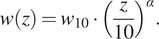
. To compute the wind power generation of each turbine, we feed the GP wind speed predictions at the turbine locations into turbine power curves. An example of such a curve is given in Figure 3. We choose a suitable power curve for each turbine we model by mapping the turbines from the Python library windpowerlib (Haas et al., Reference Haas, Krien, Schachler, Bot, Zeli, Maurer, Shivam, Witte, Rasti, Seth and Bosch2024) to the static turbine data provided by Manske and Schmiedt (Reference Manske and Schmiedt2023). For each installed turbine in the German database, we choose the turbine in windpowerlib whose capacity is closest to the actual installed capacity. To model past yearly wind power generation, we account for all turbines installed in or before the respective year. For future wind power generation, we account for all turbines in the database whose commission date is 2024 or earlier.
$ \alpha =\frac{1}{7} $
. To compute the wind power generation of each turbine, we feed the GP wind speed predictions at the turbine locations into turbine power curves. An example of such a curve is given in Figure 3. We choose a suitable power curve for each turbine we model by mapping the turbines from the Python library windpowerlib (Haas et al., Reference Haas, Krien, Schachler, Bot, Zeli, Maurer, Shivam, Witte, Rasti, Seth and Bosch2024) to the static turbine data provided by Manske and Schmiedt (Reference Manske and Schmiedt2023). For each installed turbine in the German database, we choose the turbine in windpowerlib whose capacity is closest to the actual installed capacity. To model past yearly wind power generation, we account for all turbines installed in or before the respective year. For future wind power generation, we account for all turbines in the database whose commission date is 2024 or earlier.
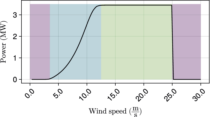
Figure 3. Turbine power curve of the Enercon E-53/800 turbine. No power is generated at very low and very high wind speeds (purple), and once the rated power has reached maximum, power is generated in all cases (green). The relationship between wind speed and power output is almost cubic in the blue part.
We compare these location-aware predictions to non-location-aware predictions using gridded data. An overview of the two approaches is given in Figure 4. For the gridded approach, we set the turbine height to the mean (78.77 m) of the 2011 turbine dataset (Manske and Schmiedt, Reference Manske and Schmiedt2023) and choose the turbine that occurs most often (E-53/800), one of the smallest turbines in the database. The gridded approach cannot account for an increasing number of turbines as the power curve is applied to each grid point, independent of the number of turbines installed. The prediction of the total power generated by either of the predictions at a time point
 $ t $
is called
$ t $
is called
 $ {p}_{\mathrm{pred}}(t) $
, which is the sum over all grid points or turbines. We perform linear bias correction by computing a factor
$ {p}_{\mathrm{pred}}(t) $
, which is the sum over all grid points or turbines. We perform linear bias correction by computing a factor
 $ f $
that ensures that the cumulative power generation prediction after 365 days
$ f $
that ensures that the cumulative power generation prediction after 365 days
 $ {P}_{\mathrm{pred}}\left(365\cdot 4\right) $
equals the power
$ {P}_{\mathrm{pred}}\left(365\cdot 4\right) $
equals the power
 $ {P}_{\mathrm{true}}\left(365\cdot 4\right) $
that was generated in the considered year
$ {P}_{\mathrm{true}}\left(365\cdot 4\right) $
that was generated in the considered year
 $$ f=\frac{\sum_{i=1}^{365\cdot 4}{p}_{\mathrm{pred}}(i)}{\sum_{i=1}^{365\cdot 4}{p}_{\mathrm{true}}(i)}=: \frac{P_{\mathrm{pred}}\left(365\cdot 4\right)}{P_{\mathrm{true}}\left(365\cdot 4\right)}. $$
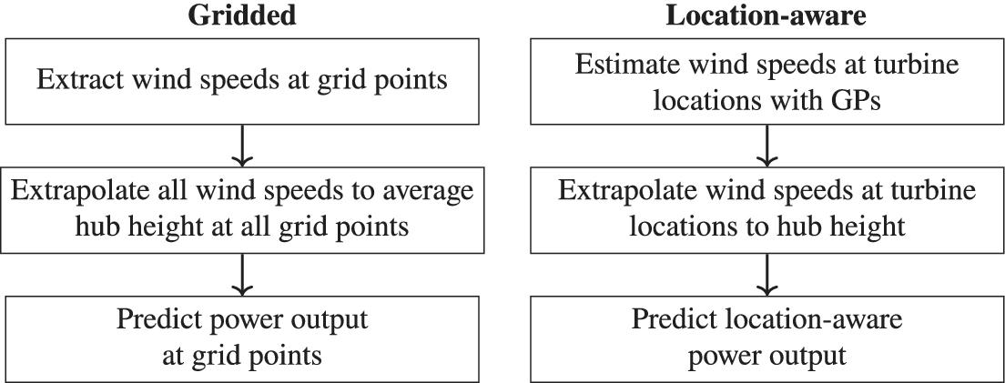
Figure 4. Overview of the gridded and location-aware approach. The gridded approach is based on gridded weather or climate data, and the predictions cannot account for turbine locations. The location-aware approach takes turbine locations into account.
This linear bias correction term accounts for dispatch (e.g., Göransson and Johnsson, Reference Göransson and Johnsson2009) and other constant biases in wind power modeling. We correct the historical projections (2011 to 2014), past projections (2015 to 2023), and future projections (starting 2024) with the actual power generation of 2011, 2015, and 2023, respectively. Bias correction is applied to both gridded and location-aware predictions in the same way. It scales the gridded and location-aware predictions, allowing for a quantitative comparison of the two predictions.
2.7. Evaluation period from 2011 to 2023
Given past data, we evaluate the methodology by comparing historical runs of GCMs from 2011 to 2014 to ERA5 and realized power generation in Germany. Furthermore, we consider different CMIP6 scenarios between 2015 and 2023. An overview of the different datasets and how they temporally overlap can be found in Figure 1. We compare the historical and scenario runs of CMIP6 to ERA5, as the latter is highly correlated with observational data (Kaspar et al., Reference Kaspar, Niermann, Borsche, Fiedler, Keller, Potthast, Rösch, Spangehl and Tinz2020) and showed better performance in forecasting wind power generation than other reanalysis datasets such as MERRA2 in previous studies (Olauson, Reference Olauson2018). As actual power generation is our variable of interest, we compare the wind power predictions from the historical runs with the power generation reported by the four different German TSOs (OPSD, 2024). After 2015, aggregated wind power generation data of these TSOs are available on the SMARD database Bundesnetzagentur (2024), which we compare to the power predictions from the climate scenario projections.
3. Results
We divide our results into three parts: 1) validation of our method through investigation of past data, 2) future wind power projections, and 3) spatial uncertainty quantification. Our results reveal that including turbine locations strongly influences multi-decadal wind power predictions. We further find that—independent of the scenario considered—the uncertainty of climate projections over Germany is higher in the coastal North than the mountainous South.
3.1. Method validation
Using GCM data and turbine locations, we predict wind power generation in Germany. For the historical period 2011 to 2014, location-aware cumulative power predictions with ERA5 overestimate wind power generation by 5.02%, and the location-aware prediction using the historical run of the MPI-ESM1.2-HR model is considered to underestimates power generation by 0.78%, see Figure 5. In both cases, the accuracy of the non-location-aware prediction is lower, with an underestimation of 9.49% and 12.51% for ERA5 and CMIP6, respectively. In the future scenarios for our region and study period, we find that the location-aware prediction based on SSP5–8.5–the worst-case reference scenario considered– is closest (+2.68%) to the actual generated power, see Figure 6. However, the climate scenario that aligns closest with the turbine location-aware prediction based on ERA5, in terms of mean absolute error, is the medium-to-high reference scenario SSP3–7.0 (Meinshausen et al., Reference Meinshausen, Nicholls, Lewis, Gidden, Vogel, Freund, Beyerle, Gessner, Nauels and Bauer2020, see Supplementary Appendix A and Supplementary Table A.1. If locations and with that, the increasing number of turbines are not considered, wind power generation is underestimated in the climate scenarios as well as ERA5. If the prediction is weighted by the number of turbines in a specific year (SSP3–7.0 + #t), wind power predictions get underestimated compared to the location-aware prediction (SSP3–7.0).

Figure 5. Power prediction using historical CMIP6 data and ERA5 relative to the actual power generated using single-output GPs. A value of 1.0 indicates a perfect prediction. It can be seen that location-aware predictions are closer to the actual power generated.

Figure 6. Power prediction relative to the actual power generated using scenarios of one climate model using single-output GPs. The first number in brackets is the accuracy of the prediction without location awareness (dotted lines), and the second is with location awareness (solid lines).
3.2. Turbine location-aware multi-decadal wind power predictions in Germany using CMIP6
We predict turbine location-aware wind power for Germany up to the year 2050 and compare location-aware to non-location-aware predictions. We present yearly results in Figure 7 and show the cumulative predictions in Supplementary Figure A.5. For 2050, location-aware predictions result in expected power generation between 87.87 TWh and 138.98 TWh; see Table 1. For the scenarios SSP1–2.6, SSP3–7.0, and SSP5–8.5, being location-aware results in lower expected cumulative power between 2025 and 2050, namely by 14.77%, 13.85% and 84.34% respectively. Only in scenario SSP2–4.5 is the cumulative location-aware power prediction 1.34% higher than the non-location-aware prediction.
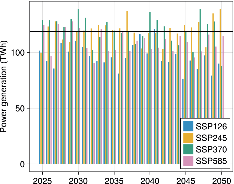
Figure 7. Yearly turbine location-aware power predictions for the different climate scenarios. The black line indicates the onshore wind power generation in 2023. On average, wind power generation in SSP2–4.5 and 3–7.0 will be a bit higher than in 2023, while SSP1–2.6 and SSP5–8.5 project lower power generation.
Table 1. Power generation predictions using the different climate scenario pathways of the MPI-ESM1.2-HR. In the 2023 persistence prediction (last row), we do not correct for the extra day in leap years

In Germany, in 2023, a total of 448,85 TWh of electric power was fed into the grid, with a relative amount of 118,78 TWh (26.46%) being wind power (Bundesnetzagentur, 2024). To contextualize the reported results, we compare the power predictions for 2050 to the expected power consumption of 506 TWh in 2050 as reported by the Federal Environment Agency (2024). The predictions of the different scenarios reveal an expected power generation between 87.87 TWh and 138.98 TWh, which is between 17.37 and 27.47% of the total power target of 2050.
3.3. Uncertainty quantification
The GP framework enables integrating the different ensemble members into the projection and quantifying the uncertainty. As only two not temporally aligned SSP runs are available, the variance per timestep of these is difficult to interpret. In our model setup, we choose to use the variance of the two model runs per scenario as noise
 $ \sigma $
(see Equation (2.1)), which results in a spatially meaningful posterior variance, see Figure 8. The results mainly reveal two insights: The normalized posterior standard deviation is higher for turbine locations closer to the coast in the North and varies more with latitude than longitude. This is in line with the hyperparameter optimization, which resulted in larger values, i.e., smoother functions of longitude compared to latitude.
$ \sigma $
(see Equation (2.1)), which results in a spatially meaningful posterior variance, see Figure 8. The results mainly reveal two insights: The normalized posterior standard deviation is higher for turbine locations closer to the coast in the North and varies more with latitude than longitude. This is in line with the hyperparameter optimization, which resulted in larger values, i.e., smoother functions of longitude compared to latitude.

Figure 8. Average posterior standard deviation at the turbine locations in 2050 for SSP1–2.6 (top left), SSP2–4.5(top right), SSP3–7.0 (bottom left), and SSP5–8.5 (bottom right). The overall pattern is similar for all scenarios, with higher uncertainties in the coastal North than in the mountainous South.
4. Discussion
Our results indicate that GCM output and turbine locations make multi-decadal wind power predictions possible. In many experiments, non-location-aware predictions differed substantially from location-aware predictions, indicating that accounting for the number and locations of turbines is crucial. Our results investigating past data reveal that for the region and time considered, turbine-location-aware power predictions using SSP3–7.0 are most similar to the predictions with ERA5 data and to the ground-truth generated power. Investigating future climate projections further reveals that the differences between the two in-between scenarios SSP2–4.5 and SSP3–6.0 and wind power generation in 2023 are minor. This indicates that wind energy will likely be a reliable power source. In general, accounting for turbine locations resulted in a smaller spread of the four climate scenarios than non-location-aware predictions, indicating that climate change could have more minor impacts on wind power generation than expected when investigating raw climate model data. Due to these minor changes in expected power generation, our results are in line with other studies (e.g., Sander et al., Reference Sander, Jung and Schindler2021, Martinez and Iglesias, Reference Martinez and Iglesias2022) and underscore that wind power and storage expansion can likely compensate for the impacts of climate change. Our results regarding the spatial uncertainty of the projections further motivate wind power expansion in the South of Germany—despite the on average lower wind speeds–as less uncertain wind conditions are to be expected. Our results reveal that the best and worst-case scenarios represent only the extremes and do not account for the full spectrum of possible outcomes. This underscores the controversial results (Schwalm et al., Reference Schwalm, Glendon and Duffy2020) by Jung and Schindler (Reference Jung and Schindler2022) and Hausfather and Peters (Reference Hausfather and Peters2020), that is the need to investigate all scenarios available and not only SSP5–8.5 and SSP1–2.6.
We will discuss some assumptions we made in this work in the following. Most of these are consequences of lacking curtailment and individual turbine data. Our linear power generation bias correction can not account for potentially changing curtailment. Generally, the value of bias correction is unclear (Maraun, Reference Maraun2016), so we decided against bias correcting wind speeds. Investigating past data reveals that the correlation between ERA5 and wind power generation is not constant, indicating changes in curtailment or technical improvement of newly installed turbines. While curtailment data is partially available (e.g., Joos and Staffell, Reference Joos and Staffell2018), most of it is confidential. Therefore, the true power generation we use to validate our results is non-optimal, as it includes curtailment and other manual interventions. The predictions generated using the gridded reanalysis dataset ERA5 are a proxy for the actual wind power potential.
Another reason for not bias-correcting wind speeds is the limited availability of hub height wind data and power data in general (compare Effenberger and Ludwig, Reference Effenberger and Ludwig2022), which often limits research in renewable energy modeling. The wind data we use is 10 m surface wind speed data, which we vertically extrapolate using a wind profile power law that has known shortcomings (Touma, Reference Touma1977). Due to the lack of data at hub heights, these extrapolated wind speeds can not be validated. Therefore, while the cumulative sum over all locations is valuable, we cannot also validate the power predictions of individual turbines. This means that our predictions are only location-aware; they are not location-specific. While vertical extrapolation could, in general, be improved (e.g., Crippa et al., Reference Crippa, Alifa, Bolster, Genton and Castruccio2021), the high complexity of the atmosphere further complicates finding or learning a better parameterization of the vertical wind profile. Another simplification we make during power prediction is using deterministic power curves. Given ground truth wind power generation data at individual turbine locations, one could, for example, learn probabilistic power curves as done in Yun and Hur (Reference Yun and Hur2021). Overall, access to wind speed observations at hub height, the corresponding power data, and theoretical wind power curves could further improve such predictions.
In future work, our setup with GPs can be used to investigate other potential turbine scenarios, which can help political decision-makers select turbine locations and expand storage capacities. Furthermore, the ability of GPs to quantify uncertainty has not been fully exploited in this study; this could, for example, be improved by using large ensembles (e.g., Olonscheck et al., Reference Olonscheck, Suarez-Gutierrez, Milinski, Beobide-Arsuaga, Baehr, Fröb, Ilyina, Kadow, Krieger and Li2023) and taking more than two ensemble members into account and adjusting the noise-level
 $ \sigma $
in Eq. (2.1) accordingly. Additionally, it would also be beneficial for uncertainty quantification to account for the differences among climate models. However, this is a very complex topic (e.g., Merrifield et al., Reference Merrifield, Brunner, Lorenz, Humphrey and Knutti2023; Morelli et al., Reference Morelli, Effenberger, Schmidt and Ludwig2025) and requires careful model selection, which is why we limit the scope of this study to the MPI-ESM1.2-HR model, motivated by Morelli (Reference Morelli2024). Future research should also emphasize validating the methodology for larger regions, which requires a lot of effort (e.g., Zhang et al., Reference Zhang, Tian, Sengupta, Zhang and Si2021), due to the lack of a common database for wind turbine installations. Additionally, our setup is promising for investigating physics-informed GP kernels (e.g., Pförtner et al., Reference Pförtner, Steinwart, Hennig and Wenger2022). In this work, we focus on a single, interpretable machine learning model. However, beyond the already discussed extensions within the framework of Gaussian processes, the insights gained regarding the value of location-aware predictions can inform future research involving more complex statistical or machine learning approaches. Additionally, systematically benchmarking location-aware models may further improve predictive accuracy and provide deeper insights into how climate change could impact future wind power generation.
$ \sigma $
in Eq. (2.1) accordingly. Additionally, it would also be beneficial for uncertainty quantification to account for the differences among climate models. However, this is a very complex topic (e.g., Merrifield et al., Reference Merrifield, Brunner, Lorenz, Humphrey and Knutti2023; Morelli et al., Reference Morelli, Effenberger, Schmidt and Ludwig2025) and requires careful model selection, which is why we limit the scope of this study to the MPI-ESM1.2-HR model, motivated by Morelli (Reference Morelli2024). Future research should also emphasize validating the methodology for larger regions, which requires a lot of effort (e.g., Zhang et al., Reference Zhang, Tian, Sengupta, Zhang and Si2021), due to the lack of a common database for wind turbine installations. Additionally, our setup is promising for investigating physics-informed GP kernels (e.g., Pförtner et al., Reference Pförtner, Steinwart, Hennig and Wenger2022). In this work, we focus on a single, interpretable machine learning model. However, beyond the already discussed extensions within the framework of Gaussian processes, the insights gained regarding the value of location-aware predictions can inform future research involving more complex statistical or machine learning approaches. Additionally, systematically benchmarking location-aware models may further improve predictive accuracy and provide deeper insights into how climate change could impact future wind power generation.
5. Conclusion
Using Gaussian processes to investigate past data from historical and scenario climate model runs, we find that multi-decadal wind power forecasting using the MPI-ESM1.2-HR model is promising. We also show that accounting for turbine locations is important and results in more accurate predictions than non-location-aware predictions. Our study demonstrates that while climate change may bring minor changes to wind power generation in Germany by 2050, wind energy will likely remain a reliable power source under most climate scenarios. Furthermore, the greater uncertainty in Northern coastal regions, compared to the South, emphasizes the importance of location-specific strategies to enhance wind power reliability in the upcoming years.
Open peer review
To view the open peer review materials for this article, please visit http://doi.org/10.1017/eds.2025.10018.
Supplementary material
The supplementary material for this article can be found at http://doi.org/10.1017/eds.2025.10018.
Acknowledgements
The authors thank the International Max Planck Research School for Intelligent Systems (IMPRS-IS) for supporting Nina Effenberger. We acknowledge support by Open Access Publishing Fund of University of Tübingen. The authors also thank Luca Schmidt and the anonymous reviewers of the Neurips 2024 Climate Change AI workshop for valuable feedback on earlier versions of the manuscript.
Author contribution
Conceptualization: N.E.; N.L. Methodology: N.E.; N.L. Data curation: N.E. Data visualisation: N.E. Writing original draft: N.E. All authors approved the final submitted draft.
Competing interests
The authors declare none.
Data availability statement
All data is open-source, all processed data is on Zenodo (Effenberger and Ludwig, Reference Effenberger and Ludwig2025). The code is available on https://github.com/NinaEffenberger/turbine-predictions-germany. CMIP6 data (Müller et al., Reference Müller, Jungclaus, Mauritsen, Baehr, Matthias Bittner, Bunzel, Esch, Ghosh and Haak2018) can be downloaded from the ESGF node (ESGF, 2024). Power generation for earlier years can be downloaded for the individual German TSOs (OPSD, 2024); for later years, they are available through the SMARD database (Bundesnetzagentur, 2024). Turbine data is provided by Manske and Schmiedt (Reference Manske and Schmiedt2023). The reanalysis dataset used is ERA5 (Hersbach et al., Reference Hersbach, Bell, Berrisford, Hirahara, Horányi, Muñoz-Sabater, Nicolas, Peubey, Radu and Schepers2020). Turbine data is from windpowerlib (Haas et al., Reference Haas, Krien, Schachler, Bot, Zeli, Maurer, Shivam, Witte, Rasti, Seth and Bosch2024).
Ethics statement
The research meets all ethical guidelines, including adherence to the legal requirements of the study country.
Funding statement
Funded by the Deutsche Forschungsgemeinschaft (DFG, German Research Foundation) under Germany’s Excellence Strategy—EXC number 2064/1—Project number 390727645 and the Athene Grant of the University of Tübingen.


 Open access
Comments
Dear editors,
I am enclosing a submission entitled “Turbine location-aware multi-decadal wind power predictions for Germany using CMIP6” to Environmental Data Science. In this study, we use Gaussian processes to predict multi-decadal power generation in Germany using wind speeds from CMIP6. The submission derives from the ClimateChangeAI Workshop at Neurips 2024.
Our results support using CMIP6 climate model data for multi-decadal wind power predictions and highlight the importance of being location-aware. We find that wind power projections of the climate scenarios SSP2-4.5 and SSP3-7.0 closely align with actual wind power generation between 2015 and 2023 in Germany. Our location-aware future predictions up to 2050 reveal only minor changes in yearly wind power generation and larger uncertainty associated with Germany’s coastal areas in the North than Germany’s South. Therefore, our results further motivate wind power expansion in the South of Germany, where wind power is currently underutilized.
This work contributes to analyzing future German wind power potential using global climate model data. Our framework can also be easily adapted and applied to many other regions where data on turbine locations and aggregate power generation are available.
The keywords for our submission are: CMIP6, wind power, Gaussian processes, climate change.
All the data used in this study are open-source. Upon acceptance of our manuscript, we will make the datasets and study code available on GitHub. As the corresponding author, I confirm that all co-authors have approved the submission of this manuscript to Environmental Data Science and that it has not been submitted or published elsewhere.
If you require any additional information, please do not hesitate to contact me.
Sincerely,
Nina Effenberger