


Introduction
To have useful information about the material is necessary for RF and microwave engineering. Providing an accurate estimation of material property is essential in various areas, including industry, healthcare, biomaterials, and medical application. There are many techniques available for characterization of the material, such as transmission-line techniques, coaxial probes, free-space methods, and cavity resonator methods [Reference Jilani, Khan, Khan and Ali1–Reference Karaaslan, Unal, Alkurt, Deng and Abdulkarim3]. Among these techniques, the cavity resonators are particularly suitable for highly accurate characterization [Reference Cheng and Liu4]. It is to be noted here that the metal waveguide is deeply restricted due to its large dimension, bulky size, and particularly its non-integrability with other RF circuits. As planar technology has become more popular for sensors, the metal waveguide has been given place to the substrate-integrated-waveguide (SIW), which contains the advantage of planar technology and conventional waveguide [Reference Bozzi, Georgiadis and Wu5]. The resonator-based techniques are the best selection for accurate determination of the complex permittivity of low loss materials. Among resonator-based approach, the cavity perturbation technique is one of the best techniques which is used to extract complex permittivity of materials in the microwave frequency range [Reference Lobato-Morales, Corona-Chávez, Murthy and Olvera-Cervantes6]. However, conventional cavity perturbation is based on several assumptions that deteriorated the accuracy of the method. In recent years, a few of the major limitations are relaxed, which the accuracy of the cavity perturbation technique has increased significantly [Reference Jha and Akhtar7, Reference Peng, Hwang and Andriese8]. Most of these modifications are dedicated to the single-mode operation, preferably the dominant mode. While in broadband material characterization, the higher order modes have also been considered in the metal waveguide cavity [Reference Jha and Akhtar9]. Also, in [Reference Tiwari, Jha, Singh, Akhter, Varshney and Akhtar10], the conventional cavity perturbation method is modified to be suitable for the higher order modes and the measurement is done in the TE 1,0,5, TE 1,0,7, TE 1,0,9, and TE 1,0,11. Furthermore, back propagation artificial neural networks are also utilized for obtaining the complex permittivity [Reference Yang, Xin, Jiao, Zhou, Wu and Huang11, Reference Jha and Akhtar12].
Resonators are usually immersed in a mass of liquid specimens [Reference Liu and Tong13] or loaded by a microcapillary filled with samples [Reference Silavwe, Somjit and Robertson14] to gain the interaction between the liquid and the electric fields and then this interaction is reflected in scattering parameter and subsequently calculating the liquid dielectric properties. Such methods, however, suffer from low sensitivity and a considerable amount of specimens is required.
In this paper, we present a novel SIW cavity sensor which operates in 11–20 GHz frequency range, with an application for detection of dispersion property of liquids. By using internal vias and PBG, we obtained a sensitivity of 0.7%. Also, the presented SIW-based structure's Q-factor has improved significantly. Moreover, by using a winding fluidic channel, the interaction between the liquid under test and the induced electric field increased. It is important to note that unlike the method presented in [Reference Tiwari, Jha, Singh, Akhter, Varshney and Akhtar10], which restricted the detection to the higher odd modes, in the proposed approach, by using a fluidic channel, we are able to do the detection task in all the higher modes.
The present paper is structured as follows. In section “Sensor design”, the geometry of the sensor design is demonstrated and the simulation result is shown. In section “Simulation result and parametric study of the transmission coefficient”, the sensor design procedure and parametric studies via simulation modeling for the transmission coefficient are presented. The theory of the perturbation method is discussed in section “Theory”. Section “Result and discussion” contains the extracted result of complex permittivity and sensitivity. Finally, the conclusion is presented in section “Conclusion”.
Sensor design
In this section, the procedure of the SIW cavity design is discussed. The SIW structure operates in X, Ku, and K frequency band and the detailed geometry is illustrated in Fig. 1a. The substrate is Rogers RT/Duroid 5880, having a dielectric constant of 2.2 and a thickness of 1.2 mm. The effective length and width of the sensor is calculated by [Reference Wang and Cheng15]


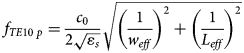
where d and s are the diameter of metalize via and spacing between two adjacent vias, l and ω are the length and width of the SIW sensor, respectively.

Fig. 1. Configuration of the final design.
The final sensor, as shown in Fig. 1, has been developed in several steps. First, a simple SIW cavity with a standard 50-ohm microstrip feedline is proposed (Fig. 2). Then, for achieving a higher Q factor and operating the proposed SIW sensor near the undercoupled mode, another microstrip transmission line with different width is added to the standard microstrip feed. Finally, by adding PBG holes around the LUT, the sensitivity of the SIW cavity has enhanced. The geometric parameters of the sensor are optimized to achieve the minimum transmission coefficient at the resonance frequency, and the detailed optimized values are presented in Table 1.
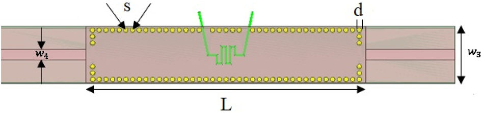
Fig. 2. Configuration of the first design.
Table 1. Parameter of the SIW cavity sensor

The PBG array with the diameter D PBG = 2 mm is created around the winding channel with a radius of 3.85 mm, and an angle between two PBG is 40°. The diameter of the internal metalized vias is 0.7 mm and the center-to-center spacing between two adjacent vias is fixed at 0.8 mm.
The proposed model is simulated by CST frequency-domain solver and the transmission coefficient (11–20 GHz) is calculated for the cavity which operates in multimode, i.e. from TE 1,0,5 to TE 1,0,11. To verify the result, HFSS and CST time-domain solvers are also used, and their results are shown in Fig. 3. Figure 3 shows that the result for both software completely agreed with each other.
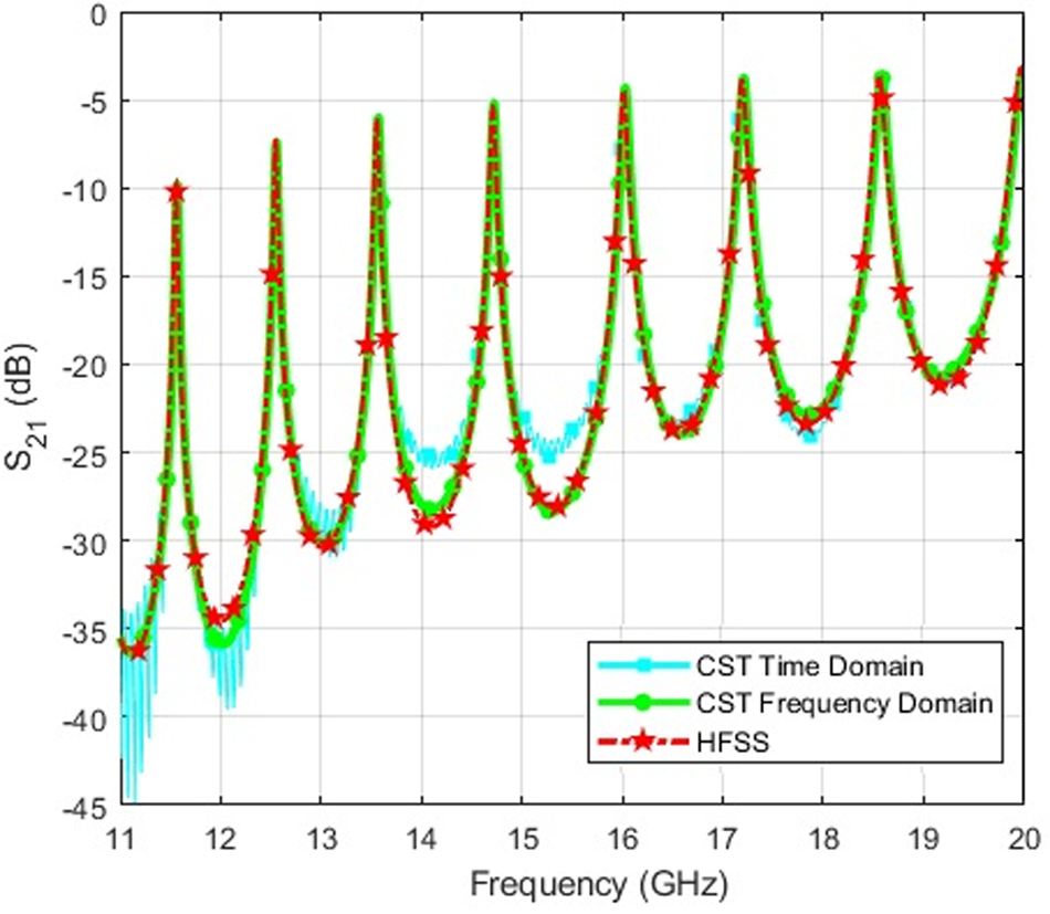
Fig. 3. Comparison between simulated S 21 of the final SIW cavity with different solver and software.
Simulation result and parametric study of the transmission coefficient
Studies and the simulation are carried out by using CST-MWS full-wave software. First, the effect of the microstrip width on the transmission coefficient has been studied. Then, the resonant frequency shift of the structure in the absence and presence of internal vias is compared. Also, the effect of PBG holes on sensor architecture and its frequency shift is parametrically studied. Herein, by gradually increasing the relative permittivity of the MUT from 1 to 20, in Fig. 4, the shift in frequency for the proposed sensor is compared with those recently introduced in [Reference Yang, Xin, Jiao, Zhou, Wu and Huang11, Reference Wei, Huang, Li, Xu, Ju, Liu and Ni16]. It is evident that for every relative permittivity of the MUT, the proposed sensor exhibits a higher frequency shift in comparison with [Reference Yang, Xin, Jiao, Zhou, Wu and Huang11]. However, this trend for [Reference Wei, Huang, Li, Xu, Ju, Liu and Ni16] is higher for the MUT's relative permittivity from 1 to 8, and the frequency shift for the proposed sensor exceeds the relative permittivity of the MUT higher than 8. Also, to show the final design's advantage, the quality factor (Q 0) and the coupling coefficient (g) of the first and final designs are compared. The unloaded factor can be calculated from 3 dB bandwidth and the resonant frequency, as:

where f H,3 dB and f L,3 dB are the high and low frequencies at 3 dB bandwidth, respectively, and shown in Fig. 5. As shown in Fig. 5, it could be observed that the quality factor of the final design has increased as compared with the first design. For the final design, the quality factor Q 0 ranged from 350 for TE 1,0,5 to 150 for TE 1,0,11. Meanwhile, the proposed feeding excites the cavity near the undercoupled mode while the standard feedline excites the cavity in overcoupled mode, which can be concluded from the fact that the modified feeding is more suitable for characterizing the material.
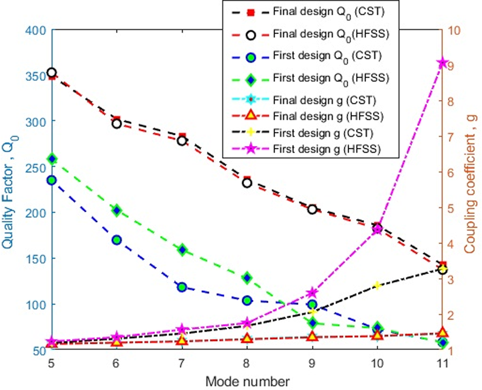
Fig. 4. Comparison between unloaded quality factor Q 0, and coupling coefficient g of the SIW cavity for final and first design.
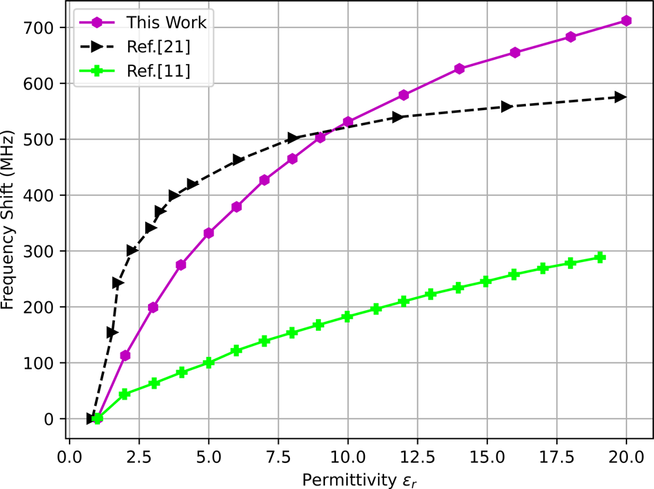
Fig. 5. Comparison between the simulated frequency shift of the proposed with that of the earlier works.
Insertion loss with different feedline width
Herein, the proposed model with different microstrip length and width is considered and the magnitude of S 21 is calculated using CST, and the result is shown in Fig. 6. Figure 6 shows the transmission coefficient concerning the variation of the length and the width of feedline changes. Specifically, S 21 of the model with l 1 = 13 and w 2 = 0.8 mm has less coupling, which improves material characterizing and these values are chosen for the feedline. Moreover, in this case, the quality factor of modes attains the highest value.

Fig. 6. Simulated transmission coefficient (S 21) of variation feedline length and width.
Transmission coefficient studies of the first design
To study the structure (Fig. 7), several samples with different permittivity values (2–4) are applied into the fluidic channel, and a considerable frequency shift is revealed in simulation, from the sensor without sample. The frequency shift corresponding to TE 1,0,6, TE 1,0,7, TE 1,0,8, TE 1,0,9, TE 1,0,10, and TE 1,0,11 is shown in Fig. 8. Also, as shown in Fig. 8, change in dielectric constant corresponds to 50 MHz resonance frequency shift on average. It is also clear from Fig. 8 that the proposed structure is more sensitive to changes between 1 and 2 since total shift is more remarkable than 85 MHz. However, in [Reference Dalgaça, Bakrb, Karadac, Ünala, Karaaslana and Sabahd17], the frequency shift concerning the dielectric change is 350 MHz on average.
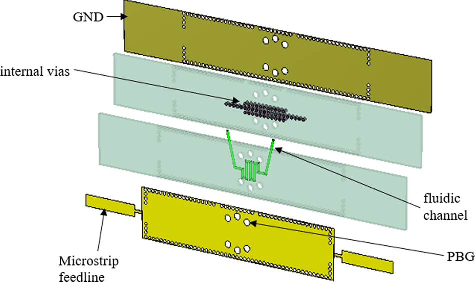
Fig. 7. Configuration of the SIW cavity 3-D view of the final design.
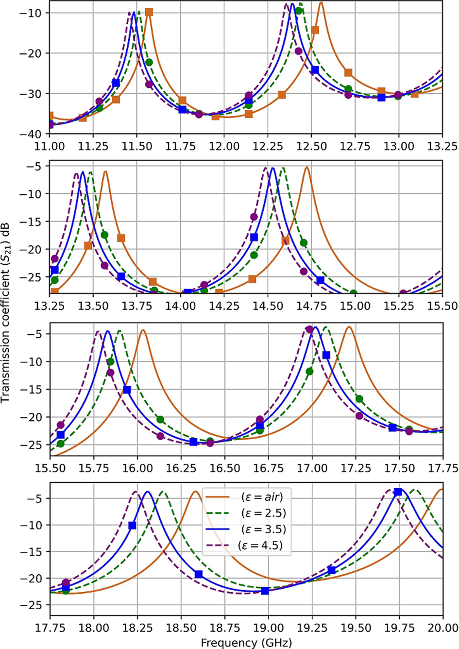
Fig. 8. Simulated transmission coefficient data for samples with different permittivity value.
Study of transmission coefficient for sensor design with and without internal vias
In order to improve the sensor sensitivity, in this step, three rows of vias have been added in the substrate, as shown in Fig. 9. As mentioned before, the height of the lateral vias is h 1 where h 1 < h. The aim of the internal vias is to increase the physical concentration of the electric field in the upper part of the substrate, where the microfluidic channel is located. Thus, the capacitive effect in this region will rise and consequently the sensitivity increases (see Figs 10 and 11) while the magnetic field remains stable in the whole substrate [Reference Niembro-Martín, Nasserddine, Pistono, Issa, Franc, Vuong and Ferrari18].
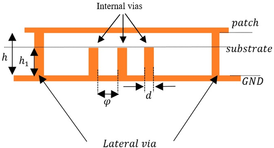
Fig. 9. Schematic cross-section view of internal via.
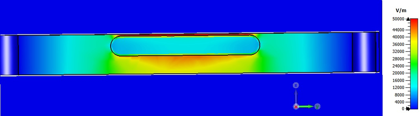
Fig. 10. Cross-section view of electric field distribution at 12.54 GHz S 21 before adding internal vias.
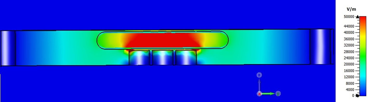
Fig. 11. Cross-section view of electric field distribution at 12.54 GHz S 21after adding internal vias.
Also, the effect of internal vias variation is studied by increasing the relative height (h 1/h) of the internal metalized vias and calculating the frequency shift when the fluidic channel is filled with an ɛ = 20 sample (Fig. 12). As shown in Fig. 12, the larger the ratio (h 1/h), the higher the frequency shift is. This phenomenon is based on increasing the capacitive coupling between the top of the internal vias and the patch layer.
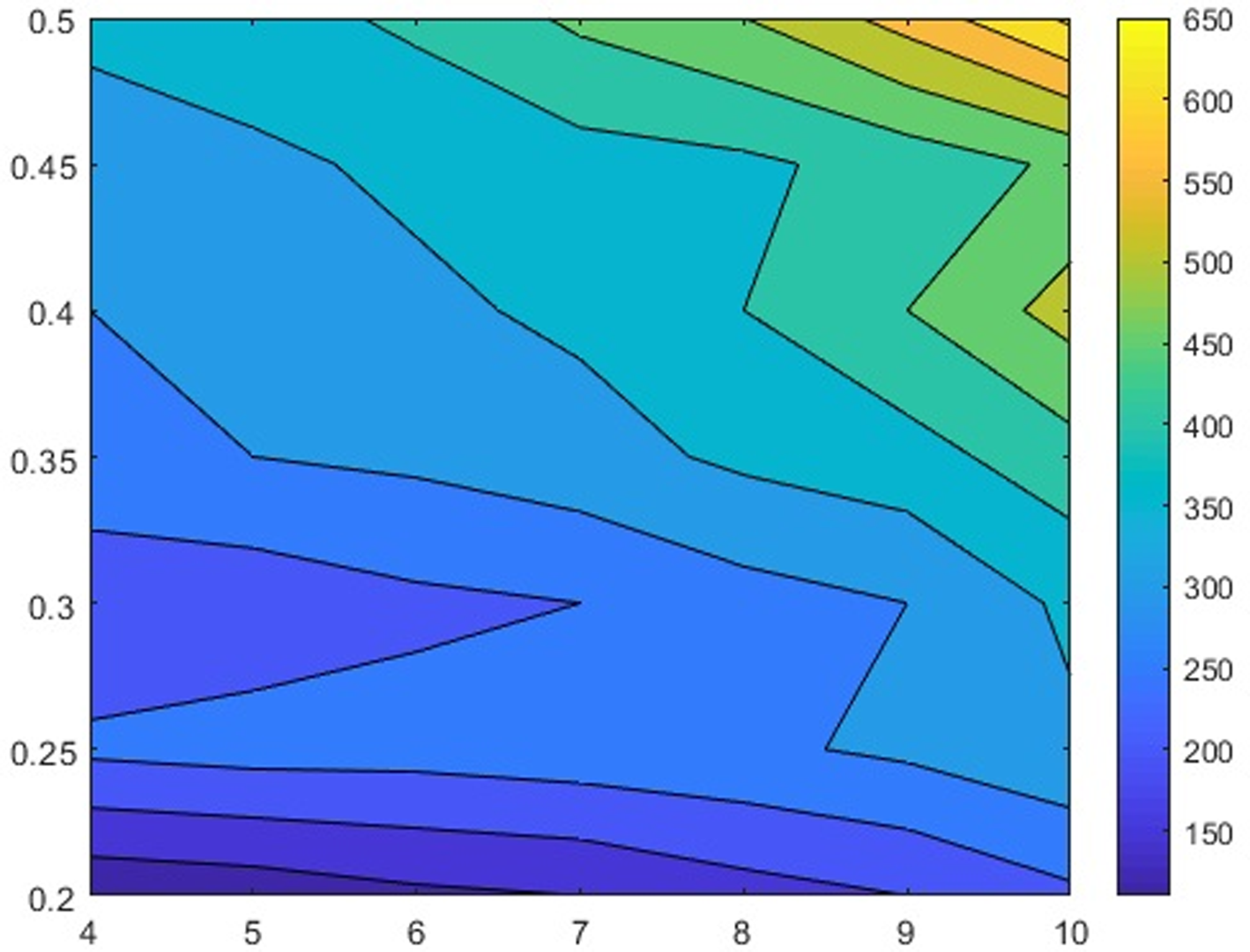
Fig. 12. Frequency shift with respect to the internal via height and operation mode variation.
Also, to have a clear understanding of the effect of vias on sensitivity, the transmission coefficient (S 21) results of the proposed sensor when the fluidic channel is filled with an ɛ = 20 sample in the presence and absence of internal vias are illustrated in Fig. 13. As shown in Fig. 13, by adding internal vias in the architecture of the sensor, the shift in frequency has increased compared with the sensor without internal vias. For instance, at TE 1,0,11, 685 MHz shift in frequency is observed for sensor with internal vias while this shift in frequency for sensor without internal vias is 323 MHz when the permittivity value changes from 1 to 20. As discussed in [Reference Niembro-Martín, Nasserddine, Pistono, Issa, Franc, Vuong and Ferrari18], adding vias in the substrate causes an increase in the effective relative dielectric constant of structure. Consequently, this leads to a decrease in the cutoff frequency of the exited modes. This phenomenon can be observed in Fig. 13. Resonant frequency for sensor with and without internal vias is 18.572 and 18.866 GHz, respectively.
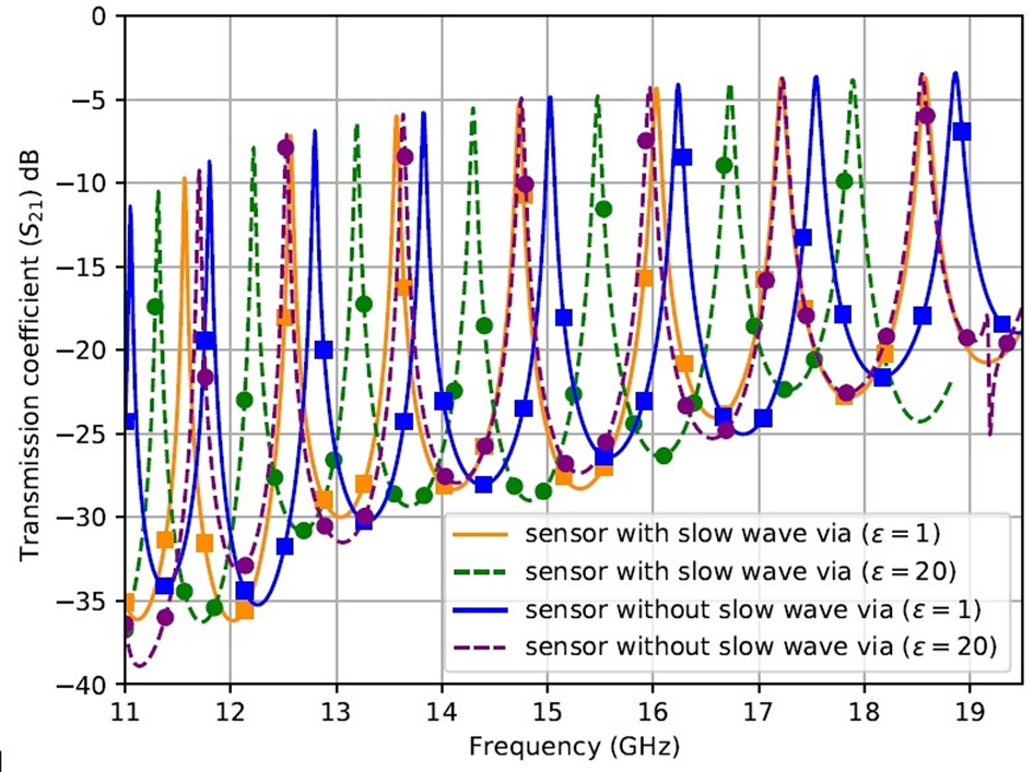
Fig. 13. Frequency shift with respect to the presence and absence of internal via for two different permittivities.
To compare the sensitivity of the SIW cavity, we consider the sensor with and without the incorporated internal vias when the same condition is applied (a channel with no sample and a channel filled with a sample (ɛr = 4)), and the resonant frequency shift is calculated. For the sensor with internal vias, the resonant frequency shift reaches 266 MHz, which the sensitivity is increased by 33%.
Transmission coefficient studies with and without PBG
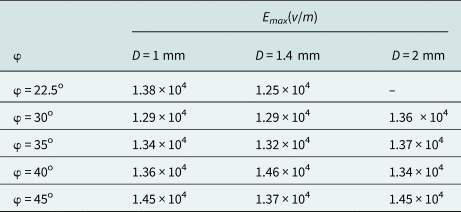
So far, we studied the sensor equipped with a new feedline and adding internal vias. In this section, PBG holes are added to the architecture of the sensor and the performance is studied under this condition. A small resonant frequency shift around 100 MHz is obtained in the transmission coefficient due to PBG holes in the structure while the magnitude of the transmission coefficient has a negligible change (see Fig. 14). Inserting the PBG in the structure reduces the substrate permittivity, which as a consequence, the resonance shift to high frequencies. Also, a parametric study is performed over the PBG hole location and diameters. As demonstrated in Fig. 15, our focus is on the radius of the PBG and the repetition angle. By varying these two parameters and recording the simulation results, the effect of each parameter on the maximum value of the electric field distribution is tabulated in Table 2.

Fig. 14. Simulated transmission coefficient (S 21) with and without PBG.
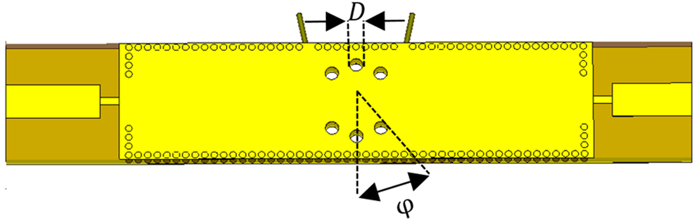
Fig. 15. The geometry of the structure for φ and diameter of PBG.
Table 2. Effect of PBG dimension and repetition angle
Herein, we consider a case in which the sample's permittivity value and the angle between two adjacent PBG's φ are simultaneously varying from 22.5 to 45o and ɛr = 1 to 10 and resonant frequency shift is calculated and depicted in Fig. 16 according to these changes. As this figure shows, the frequency shift is around 600 MHz for φ = 40o. Also, we consider the prototyped structure with and without the incorporated PBG structure and the transmission coefficient for these two situations is presented in Fig. 17. This result suggests that adding PBG holes increases the frequency shift from 330 to 695 MHz when the real part of permittivity varies from 1 to 20, respectively.
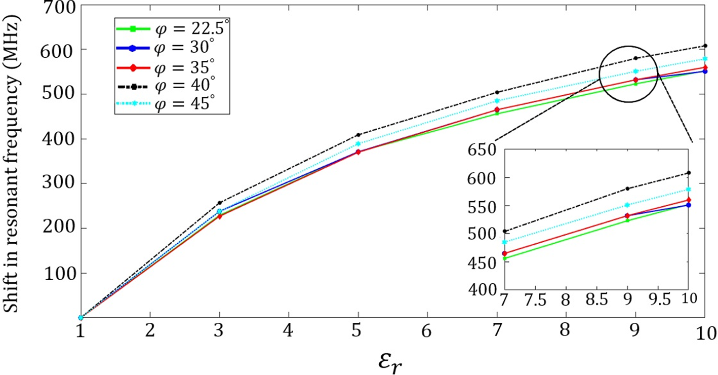
Fig. 16. Simulated frequency shift as a function of different material and φ.
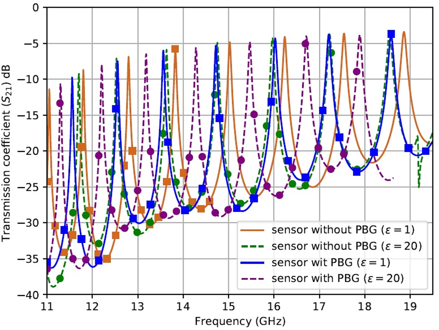
Fig. 17. Simulated transmission coefficient for different permittivity in the absence and presence of PBG.
In the next step, we impose the previous scenario and compare the sensitivity of the first design and the cavity with PBG. The frequency shift for structure with PBG is 275 MHz, which is improved by 37.5% as compared with the first design.
Transmission coefficient study of structure with lossy material
The transmission coefficient amplitude has corresponded to the loss property of the LUT at the resonant frequency. To improve the characterization, we also consider the effect of loss tangent. In this case, a liquid under test with ɛr = 2 and different loss tangents of zero to 0.5 is assumed. As shown in Fig. 18, the peak magnitude of insertion loss decreases by the increase of the loss tangent, and consequently, the Q-factor reduced. This result is due to an increase in losses, which in turn decreases insertion loss. For instance, at TE 1,0,10 when tanδ changes from 0 to 0.5, the magnitude of insertion loss is −3.72, −5.90, −7.63, −9.05, −10.25, and −11.36 dB. Also, the shift in frequency for changing the loss of the sample is negligible.
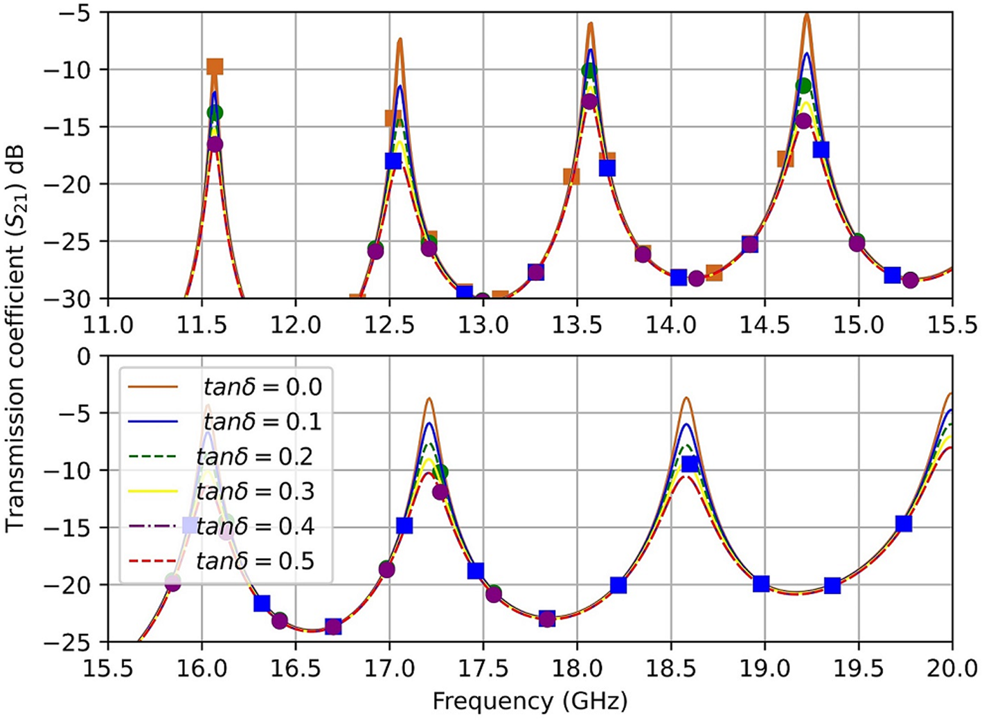
Fig. 18. Transmission coefficient magnitude concerning a sample with ɛr = 2 and different tanδ.
Parametric study for electric field
In this section, the electric field distribution in each part of the design is compared. As illustrated in Figs 19–22, the concentration of electric field in the center of the sensor where the microfluidic channel is placed shows the lower and the maximum of the electric field as 2.5 × 10⁴(V), while the maximum of the electric field in the final design enhanced up to 3.6 × 10⁴(V)(Fig. 22). By implementation of new feeding in our design, impedance matching gets better and increases the electric field concentration (Fig. 20). Then, adding the internal vias in the substrate, as mentioned before, would affect the electric field distribution and concentrate it in the upper part of substrate (Fig. 21). Finally, the creation of the PBG holes causes a wave encapsulation. This is due to that the wave is trapped and enclosed and stop the propagation of the wave in the cavity. This phenomenon increases the electric field concentration in the structure [Reference Jafari and Ahmadi-Shokouh19].
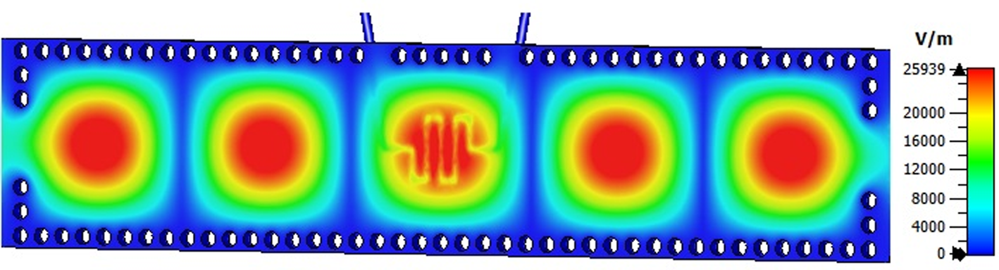
Fig. 19. Electric field distribution at TE 1,0,6 first design.

Fig. 20. Electric field distribution at TE 1,0,6 sensor with new feedline.

Fig. 21. Electric field distribution at TE 1,0,6 internal vias implementation with new feedline.

Fig. 22. Electric field distribution at TE 1,0,6 internal vias and new feedline implementation with PBG holes.
Theory
Cavity perturbation technique uses changes in resonant frequency and quality factor of a cavity as a signature to calculate complex permittivity of material placed at the maximum electric field position. In the standard SIW cavity, the formula is given as [Reference Jha and Akhtar20]


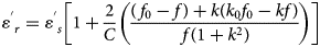
where f 0 and Q 0 represent the resonant frequency and quality factor of empty cavity and f and Q are the resonant frequency and quality factor of the filled cavity, respectively. Also, the symbols $\varepsilon _{\;s}^{\rm ^{\prime}}$ and $\varepsilon _{\;r}^{\rm ^{\prime}}$
 , respectively, represent the relative permittivity of the substrate and liquid. However, $\varepsilon _{\;s}^{\rm \prime\prime }$
 and $\varepsilon _{\;r}^{\rm \prime\prime }$
 are the imaginary part of the substrate and liquid. Moreover, V c and V s correspond to the volume of the cavity and microfluidic channel.
Although (5) and (6) accommodate the substrate permittivity, still these equations are based on several assumptions which are relaxed [Reference Jha and Akhtar9] and a new shape factor is proposed (8), where k x = mπ/w eff and k z = pπ/l eff, respectively, correspond to the wave number along the x − and z − directions and the expression for complex permittivity according to this shape factor is given as


where r is the radius of the fluidic channel.
Even though equations (8) and (9) accommodate the mode number and complex permittivity of the substrate, there is still another limitation. Equation (8) and (9) are more suitable for metal cavity due to ASTM standard that the quality factor of metal cavity is almost as high as 5000 and the term 1/Q is negligible and neglected in the equations. Moreover, in the SIW cavity, the quality factor is much lower than the metal cavity, so a new set of expression is given in (10)–(12) to relax this limitation [Reference Tiwari, Jha, Singh, Akhter, Varshney and Akhtar10].
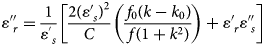

where k = 0.5(1 − |S 21|)/Q and $k_0 = 0.5( {1-\vert {S_{{21}_0}} \vert } ) /Q_0$ .
.
The abovementioned equations are considering not only the mode number but also the effect of low Q-factor in the SIW cavity. It is to be noted here that (11)–(13) are mainly originated from conventional cavity method where the electric field before and after perturbation is the same. Due to this fact that modification in the shape factor is necessary which is given in (14) [Reference Tiwari, Jha, Singh, Akhter, Varshney and Akhtar10]

where k x = (mπ/w eff)(f/f 0)x, k z = (pπ/l eff)(f/f 0)x and the values of x are calculated and reported in [Reference Tiwari, Jha, Singh, Akhter, Varshney and Akhtar10].
Result and discussion
To examine each expression's accuracy for determination of complex permittivity in our proposed structure, a mixture of cyclohexane (ɛr = 1.9798 + j0.009899) and methanol is used as samples. In this study, two liquids, i.e. cyclohexane (non-dispersive) and methanol (dispersive) are assumed. The first-order Debye model calculates the complex permittivity of methanol (15) [Reference Abeyrathne, Halgamuge, Farrell and Skafidas21].

where ɛ∞ is the permittivity at the infinite frequency, ɛs is the static permittivity, ω is the angular frequency, τ is the relaxation time. The proportions of the mixed samples vary from 1:1 to 15:1; for the 1:1 ratio, the values of $\varepsilon _r^{\prime}$ changes from 3.302 to 2.568 and the $\varepsilon _r^{\prime \prime}$
 changes from 2.48 to 2.92 in the sensor operating frequency (11–20 GHz). For the ratio 1:15, the values of $\varepsilon _r^{\prime}$
 changes from 2.133 to 2.056 and the $\varepsilon _r^{\prime \prime}$
 changes from 0.257 to 0.296 in the frequency range of 11–20 GHz. The values are calculated by the Maxwell–Garnet approximation formula. After that, by inserting these mixtures in the channel, the simulated transmission coefficient is recorded for each mixture. Then the resonant frequency and Q-factor corresponding to each mixture value for TE 1,0,6 to TE 1,0,11 modes are calculated. The values of the quality factors and resonant frequency are then used to calculate the complex permittivity using the expression which is mentioned in section “Theory”. Then, they are compared with each other.
Moreover, to obtain another mathematical relationship between the resonant frequency of the sensor and the relative permittivity, the SIW cavity response to the various permittivity samples is used. Then, the variation in resonant frequency plotted against the relative permittivity of the sensor, and with the help of MATLAB, a curve fitting is carried out to establish a relation based on simulation data and the fitting function to have the min-square error value. The expression given in (16) is finally obtained using this procedure for estimation of the real part of the permittivity of the LUT, as shown in Fig. 23 at TE 1,0,10 mode, for instance.
where f is the resonance frequency (GHz), a = 9.82 × 10¹⁵, b = −1.47, c = 1.059 × 10¹⁶, and d = 1.474 are the coefficients.

Fig. 23. Curve fitted for TE 1,0,10 mode.
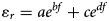
Herein, the calculated complex permittivity of four different methanol and cyclohexane mixture ratios from the simulation is compared and plotted in Fig. 24. As shown in Fig. 24, the value obtained with (11) and (12) are closer to the true value which is calculated with the Maxwell–Garnet formula (True) than other formulas as expected. Also, the percentage of error with respect to each mixture ratio is plotted in Fig. 25. As shown in Fig. 25, the maximum error in the real and imaginary part of permittivity is dedicated to equations (5) and (6). This is due to that these equations are based on several assumptions. However, equations (11) and (12) have the least percentage of error as in these equations the assumptions have been relaxed.
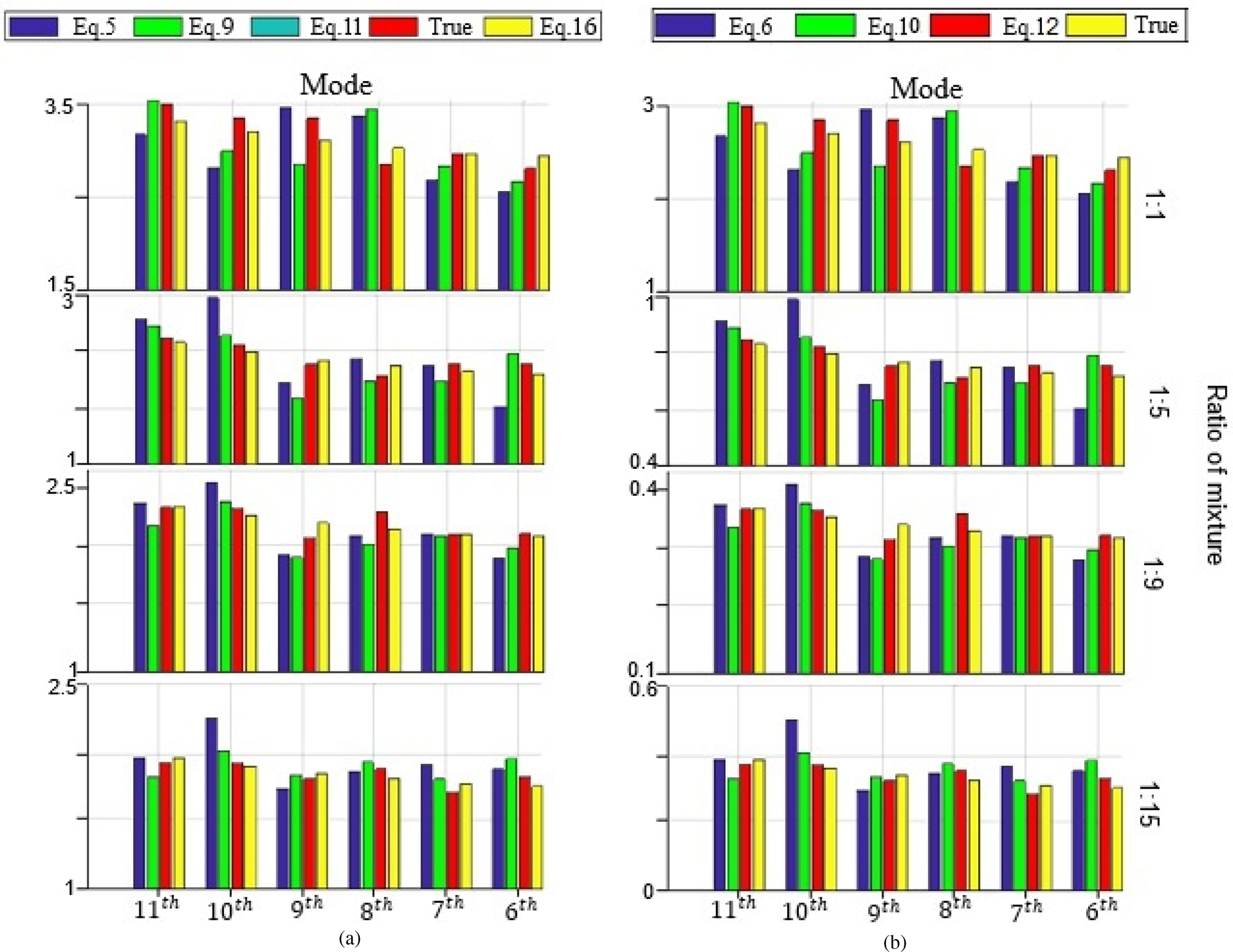
Fig. 24. Comparison of the (a) real and (b) imaginary part of permittivity data obtained using various methods.
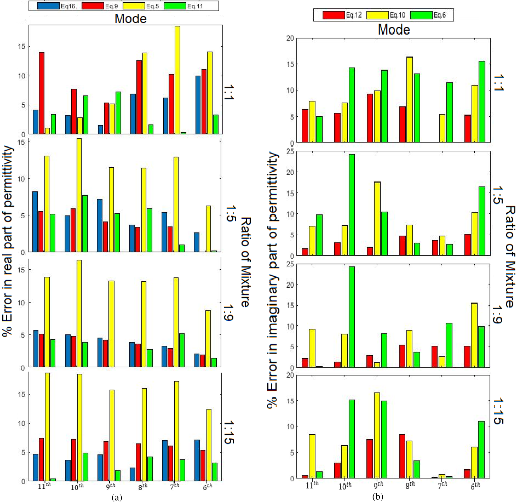
Fig. 25. Comparison of % error in (a) real and (b) imaginary part of permittivity using various techniques.
Sensor sensitivity
In this section, the fractional changes in resonant frequency for the different liquid samples are simulated and plotted in Fig. 26. As shown in this figure, with three lines, the curve of fractional changes in resonance frequency is piecewise linearly approximated which are l 1, l 2, and l 3. It can be concluded that the slope of the l 3 is higher than the other two lines, which means that sensitivity of the proposed sensor in the region where LUT has low relative permittivity value (1 < ɛr < 5) is exceptionally high compared with higher permittivity values. This excellent sensitivity performance enables the proposed sensor to easily discriminate two liquids with very close permittivity value or detect tiny changes of permittivity value. Also, in Table 3, a summary of the comparisons between this work and other recently published works in terms of sensitivity is presented. To have a fair comparison, all the calculated sensitivities of these sensors are based on the following equations [Reference Jafari and Ahmadi-Shokouh19]


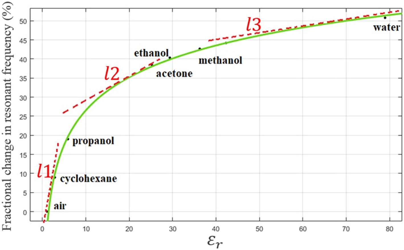
Fig. 26. Plot of the sensitivity as a function of $\varepsilon _r^{\rm ^{\prime}}$ .
.
Table 3. Comparison of recently published works and this work

Thus, the sensitivity of the sensor is obtained at 0.7%.
Conclusion
In this paper, a planar microwave sensor for liquids taking advantage of a novel SIW-based cavity has been developed. The sensor design is studied using the full-wave simulator, the CST, and detailed analyses have been carried out to enhance the sensitivity while tolerating some error in permittivity. The sensor is equipped with a winding microfluidic channel to enable the sensor to work in higher modes. The proposed technique can find its potential applications under those situations where only a small amount of liquid sample is available and illustrate an advantage over its counterparts. Also, the perturbation method is used for calculating the complex permittivity of dispersive liquids. The different mixture ratio of methanol and cyclohexane is used to evaluate the perturbation method's accuracy, and retrieved complex permittivity is presented. Moreover, the accuracy of each technique in terms of the percentage of error is presented. All the simulation and results show that the performance of the proposed SIW in terms of sensitivity has been enhanced. Also, the proposed sensors could be integrated with a portable microwave circuit.
 Kianoosh Kazemi was born in Shiraz, in 1995. In 2017, he received his Bachelor's degree from Shiraz University in Electrical Engineering. In 2019, he obtained his Master's degree from the Amirkabir University of Technology (Tehran Polytechnic), Tehran, Iran. His research interests are microwave measurement and microwave sensor.
 Gholamreza Moradi received his B.Sc. in Electrical Communication Engineering from Tehran University, Tehran, Iran in 1989, and the M.Sc. in the same field from Iran University of Science and Technology in 1993. Then he received his Ph.D. degree in Electrical Engineering from Tehran Polytechnic University, Tehran, Iran in 2002. His research areas include applied and numerical electromagnetics, microwave measurement and antenna. He has published more than 70 journal papers and has authored/co-authored seven books in his major. He is currently an Associate Professor with the Electrical Engineering Department, Amirkabir University of Technology (Tehran Polytechnic), Tehran, Iran.
 Ayaz Ghorbani received the Postgraduate Diploma, M.Phil., and Ph.D. degrees in Electrical and Communication Engineering and the Ph.D. degree from the University of Bradford, Bradford, UK, in 1984, 1985, 1987, and 2004, respectively. Since 1987, he has been teaching various courses with the Department of Electrical Engineering, Amirkabir University of Technology, Tehran, Iran. He has authored or co-authored more than 100 papers in various conferences as well as journals. Dr. Ghorbani received the John Robertshaw Travel Award and the URSI Young Scientists Award from the General Assembly of URSI, Prague, Czech Republic, in 1990. He was a recipient of the Seventh and Tenth Khwarazmi International Festival Prizes, in 1993 and 1995, respectively, for design and implementation of an anti-echo chamber and microwave subsystems.


