


A dramatic feature of nineteenth- and twentieth-century agricultural development in the Midwest and Southeast United States was the application of drainage technologies to remove water from saturated lands (see, e.g., M. Bogue Reference Bogue1951; A. Bogue Reference Bogue1963). A significant portion of the United States, including the upper Midwest, the Mississippi River Basin, and the eastern Coastal Plain, has naturally wet soils, and of the 215 million acres of wetlands estimated to exist in the contiguous United States at colonization, 124 million had been drained by 2019, with 80–87 percent drained for agricultural purposes (McCorvie and Lant Reference McCorvie and Lant1993; Tiner Reference Tiner1984).Footnote 1 Without drainage, much of the present-day Corn Belt, in Ohio, Indiana, Illinois, Iowa, and Minnesota, would be ill-suited for agriculture.
Drainage ditches, combined with subsurface drain tile (first used in Upstate New York in 1835 and adopted across the upper Midwest in the following decades) made drainage economical for widespread adoption. Some of the drainage was carried out over broad areas of swampy and submerged land—like the 25-mile by 100-mile Great Black Swamp, which in the 1850s, drained into Lake Erie at modern-day Toledo. Draining also occurred on a smaller scale in undulating fields in Indiana, Illinois, and Iowa that were only partially or seasonally submerged. Settlers in these areas began farming higher, drier ground first and, over time, converted and drained lower swales into additional farmland.
The majority of American lands with naturally wet soils are either in the upper Midwest, the result of glaciation, or in the lower Mississippi River Basin and Southeast on the low-lying coastal plain. Across the United States, around 20 percent of improved agricultural production (by area and value) and around 38 percent of corn production now occurs in counties with high natural soil wetness, which benefit from drainage. Recognition of the value of drainage investment came early. In 1880, it was estimated that drainage of unimproved wetlands increased sale value by a factor of five (Prince Reference Prince2008). Yet capturing this increased value typically required significant coordination among neighboring landowners, which was initially absent.
In this paper, we examine the coordinating mechanisms of drainage management districts. Empirically, we establish how state legislation allowed for the creation of drainage districts, thus enabling the coordination necessary for broad-scale drainage investment. While drainage typically required coordination over areas of several square miles—640 acres to the square mile—farms in the wet prairie counties were smaller, around 150 acres, due to both increasing costs of monitoring labor on larger farms and government land allocation policies (Allen and Lueck Reference Allen and Lueck1998; Prince Reference Prince2008). Drainage districts allowed landowners to retain rights to operate their farms at the scale that economic factors dictated, while ceding one property right “stick”—drainage—to a locally elected body. By granting districts taxing and eminent domain authority, drainage district laws provided a sufficient legal structure for collective investment.
Our empirical approach relies on within-state heterogeneity in the value of drainage, as dictated by natural soil wetness, to identify the effect of enabling legislation for districts. By 1920, the first year when drained acreage was systematically surveyed in the U.S. Agricultural Census, and after all states had passed drainage district legislation, 52.6 million acres had been drained across the United States. Most of the drainage (64 percent) took place in the 18 percent of counties we classify as having high natural soil wetness. Using a difference-in-difference approach, we show that counties with naturally wet soil saw increases in both improved acres and land value relative to drier counties in the same state after the passage of drainage district legislation. In naturally wet counties, drainage district legislation was capitalized into 20 percent to 37 percent higher land values, resulting in an aggregate 10 percent increase in U.S. farmland value.
Variation in the topography across naturally wet counties provides further evidence of the importance of coordination. Among wet counties, those with rougher topography do not require drainage districts because there is enough variation in elevation for farmers to drain their lands to existing streams directly without coordinating with adjacent landowners. At the other topographical extreme, drainage in wet but flat counties often requires complex coordination beyond the district level. In this latter category, drainage districts provide insufficient coordination. Our empirical analysis finds strong evidence of the anticipated heterogeneity in treatment effect across topographical extremes, along with the effectiveness of drainage districts across the broad topographical middle ground.
Primack (Reference Primack1963) appears to be the only mention in the economics literature regarding the coordination problems of drainage and the lack thereof in some instances. While he notes that some areas that could benefit from drainage did not require coordination beyond the boundaries of individual farms, he does not distinguish topographically, as we do, between areas that were drained with district-scale coordination and those for which the scope of coordination exceeded the capabilities of districts. Because comprehensive data on district formation are not available, we rely on an intent-to-treat approach to empirically show that the passage of enabling legislation led to an increase in improved acres and land value. We supplement our data analysis with institutional evidence to demonstrate that the coordination afforded by drainage district legislation triggered widespread investment. We provide a rich historical narrative of the formation of districts in one state, Illinois, to shed light on why states passed drainage laws when they did and who supported the statewide legislative and local district formation efforts.
Our work contributes to the literature on the relative roles of capital, technology, and institutions in the development of agriculture in the Midwest. The roles of capital and technology in agriculture have been discussed by economic historians for much of the past century. Several technological innovations were critical to the development of modern American agriculture, notably: railroads, which increased market access (Donaldson and Hornbeck Reference Donaldson and Hornbeck2016; Atack and Margo Reference Atack and Margo2011); mechanization, which allowed intensive application of power to farming (see Olmstead and Rhode (Reference Olmstead and Rhode2001) on the impact and diffusion of the tractor); and new seed varieties (Griliches Reference Griliches1957; Olmstead and Rhode Reference Olmstead and Rhode2011). Drainage differed from these innovations in that it represented the precondition work of creating farmland, similar to land-clearing and fencing (see the discussion in Primack (Reference Primack1963) and Reference HornbeckHornbeck (2010)). Drainage also differed from investments that occurred on a farm-by-farm basis, such as tractors, clearing, fencing, and new seed varieties, in that drainage investment often required coordination and novel governance institutions (as well as technical innovations in drain tile and excavation). In this historically significant period of American development, we document the importance of the transaction costs of collective action and the institutional innovation that addressed them.
GEOLOGY, TECHNOLOGY, AND DRAINAGE ECONOMICS
Agricultural Drainage
The macro-determinant of need for drainage in the United States is geology. The pre-Wisconsin and Wisconsin glaciations deposited swaths of flat, fertile soil across the upper Midwest. Figure 1 shows the high correspondence between drained acres in 1969 and the limit of the Wisconsin Ice Sheet, and to a lesser extent, earlier ice sheets that extended farther south. In the Southeast, the flat coastlines of the Atlantic Ocean and Gulf of Mexico seabeds have received repeated alluvial deposits from rivers, and rising and falling sea levels have deposited flat layers of marine sediment. Today, these flat coastal plains include the Texas Gulf, the Mississippi River Valley up to Illinois, and almost all of Florida and the eastern seaboard. Drainage in the Southeast corresponds closely to these plains.

Figure 1 DRAINAGE AND GEOLOGY
Notes: Map of the eastern United States showing the glaciated region by the extent of glacial advance, the coastal plain and Mississippi River Delta regions, and the total acres drained in 1969 shifted to 1910 county boundaries using area-weighted crosswalks.
Sources: Authors’ drawn map using data from National Atlas of the United States (2005), United States Environmental Protection Agency, and the National Historical Geographic Information System.
In wet and poorly drained soils, excess water in the root zone of cultivated crops can prevent the absorption of oxygen and drastically reduce yields or kill the plants entirely. Water tables can be lowered if nearby drainage provides a pathway for water out of the plant root zone. Since Colonial times, open ditches have been dug to remove excess standing water and to lower water tables. The earliest attempts at drainage in the Midwest, in 1818, were of this type (Prince Reference Prince2008, p. 205). However, ditches proved impractical for agricultural production in many cases. The ditches themselves, typically three to five feet deep, were labor-intensive and, because they bisected fields at frequent intervals, they reduced the available land surface and made planting and harvesting difficult. Methods for draining water while maintaining the integrity of the land surface via underdrainage were required for practical use.
Subsurface drains of various materials including stones, poles, and logs, were utilized in urban settings throughout the nineteenth century, but were broadly uneconomical for agriculture. Other methods, such as buried brush drainage and mole drainage, where a thin leg attached to a torpedo-shaped implement is dragged through the ground, were inconsistent, and their effectiveness declined within a few years of first use.
The technology that ultimately replaced open ditches in much of the country was the installation of drain tile. Installing drain tile involved digging a trench in which flat clay tiles were laid end to end and covered with a second, inverted-V, layer of tile, creating a porous water channel. The tile was then covered again with soil. The resulting subterranean channel drained water above it down to its level, typically four feet below the surface. Unlike open ditching, installed tile was invisible and allowed farming above it.Footnote 2
Drain tile was not uniformly adopted, and its suitability varied over space and time. Tile was well-suited for use in the glaciated regions of the Midwest but was not as successful on the Atlantic Coastal Plain and Mississippi Delta, where the need for additional investment in levees and pumping, as well as challenges related to flat topography near sea level, limited its effectiveness. These regions developed drainage using a combination of in-field ditching, levee systems, pump houses, and tile in select areas.
Drain tile allowed subsurface drainage on the farm, but it was not useful unless the water had somewhere to go, typically into a network of off-farm drainage ditches. This required coordination, initially to solve free-rider and holdout problems that arose in the construction of multi-user ditches. Coordination was also required once a drainage network was established because maintenance of an individual farm’s drain tile had off-farm effects. Clogged drain tile on one farm could cause flooding on upstream farms in the network.
While digging ditches is an iconic example of low capital intensity production, advances in digging technologies paralleled those in the manufacture of drain tile itself.Footnote 3 Such advances beyond men and shovels included the development in the 1880s of the dipper dredge, the horse-drawn Pratt Ditch Digger, and the Blickensderfer Tile Drain Ditching Machine. The latter could dig a four-foot ditch in only one pass, “powered by a single horse, one man, and one boy” (Yannopoulos et al. Reference Yannopoulos, Grismer, Bali and Angelakis2020, p. 1781). Application of fossil fuel power followed in 1892 with the introduction of the steam-powered Buckeye Trencher. In 1908, gasoline-powered internal combustion engines began to replace steam engines, as they did in tractors (Olmstead and Rhode Reference Olmstead and Rhode2001). In the early twentieth century, efficient dragline excavators came to replace dredges.
Like investment in agricultural production generally, the development of drainage was shaped by local fertility and climate, as well as input and output prices. For instance, the panic of 1873 and subsequent fall in farm prices reduced demand for drainage, while emerging transportation networks lowered the cost of moving tile, increasing the cost-effectiveness of drainage investment. As we discuss in detail in the next section, our empirical approach sidesteps much of this heterogeneity in adoption timing and location by focusing on the effects of drainage districts and through the inclusion of county and state-by-year fixed effects.
The Economics of Drainage and Coordination
In the upper Midwest prior to 1880, unimproved wetlands sold for an average of $7 per acre (ranging from $2–$12); once drained, the sale price could increase by a factor of five (Prince Reference Prince2008). Drainage was costly, however. Hewes and Frandson (Reference Hewes and Frandson1952) noted in their account of Story County, Iowa, that at the time of settlement in 1860, and for several decades afterward, the cost of tiling exceeded the price of undrained land.Footnote 4
As technology evolved and costs declined, economic incentives to drain and fully utilize lands with naturally wet soils emerged, providing evidence of direct capitalization of land improvements into land values. Because of the cost of drainage, land with wet soils was developed later. After 1880, declines in the cost of tiling drove an increase in the derived demand for its complementary input, unimproved swampland. The price of undrained swampland increased rapidly, to an average of $25 per acre (ranging from $13–$40), with drained land commanding $60–$70 per acre, a premium in the neighborhood of the cost of tiling estimated at $35 per acre (Prince Reference Prince2008).
Drainage investment, however, was generally not effective on a small scale. Drainage projects required coordination across hundreds or thousands of acres as well as new ditches, levees, and embankments on private lands (Wright Reference Wright1907; Prince Reference Prince2008). While common law was interpreted in many states, including Iowa and Illinois, as providing farmers the right to allow water outflow onto neighboring properties, the geographic scope of drainage benefits and costs created the potential for conflict. Bogue (Reference Bogue1963) uses the diaries of a nineteenth-century Illinois farmer, Croft Pilgrim, to illustrate:
Pilgrim’s earliest venture in tiling disrupted the harmony of the neighborhood. No sooner was the drain completed than his neighbor Tom Mellor dammed the outlet, claiming that the tiling system was flooding his fields. Thus in 1876 began a long-drawn-out litigation, which started in the court of the local justice of the peace and moved ultimately into the district court. After a series of decisions and appeals, the case still stood on the docket at Toulon, the county seat, in 1882, and by this time had cost Croft Pilgrim several hundred dollars.
Coordination problems among neighbors combined with large minimum scales of drainage projects, limited private investment in drainage to large landowners. Owners of farms in Illinois ranging in size from 3,000 to 17,000 acres privately undertook tiling (and, in some cases, the construction of tile factories). For the average smallholder farm, which in the upper Midwest in 1880 was about 150 acres, the necessary scale of drainage investment exceeded farm size by one to two orders of magnitude (Prince Reference Prince2008).
While the consolidation of smallholdings by large landowners capable of coordinating drainage investment offered one potential solution to the challenges of drainage, consolidation brought costs as well. Smallholders in the Midwest generally relied on family labor, where agency costs were low, and they could readily adjust efforts in response to price signals. By contrast, large landowners required external labor, leading to misaligned incentives between owners and hired labor that resulted in additional monitoring costs (Allen and Lueck Reference Allen and Lueck1998).
Some entrepreneurial landowners tiled their land and then converted it into smaller farming units of 80–160 acres, which were then sold or rented (Prince Reference Prince2008). These attempts at private solutions, however, were limited in area and impact. One key constraint was access to capital (Bogue Reference Bogue1951). In addition, for farms already held by smallholders, the transaction costs involved in consolidation, tiling, and reparcelization were high. For existing smallholders, who lacked consolidated ownership at the scale required to justify an individual drainage project, coordination was essential.
A 1907 report to the U.S. Senate on the status of Swamp and Overflowed Lands in the United States by Wright (Reference Wright1907) described the coordination problem faced in reclaiming these lands. The initial problem facing owners of swamp lands and other poorly drained areas was the coordination needed to invest in the local public goods required for reclamation. Olson (Reference Olson, Eatwell, Milgate and Newman1989) provides a useful framework for understanding the difficulties of solving this coordination and investment problem of collective action. Each farmer can be made better off from drainage investment, yet each also has an incentive to free ride on the investments of others, and one farmer’s actions can negatively affect another. Collective action in drainage requires a mechanism by which farmers agree to cooperate.
Ostrom (Reference Ostrom1990) provides insight into the settings where local groups can successfully cooperate in managing natural resources. Relevant to this work is her finding that local groups are often successful at such management, even when central governments fail. In describing her design principles for successful organizations, Ostrom suggested that the right to organize locally be recognized by the central or local government, with decisions nested within local organizations. Ultimately, it was the drainage district that provided local landowners with the tools to undertake the collective investment suggested by Olson (Reference Olson, Eatwell, Milgate and Newman1989) in a manner consistent with the nested structure described by Ostrom (Reference Ostrom1990).
The Drainage District
From a modern governance perspective, a drainage district is one of many examples of a special district, which is commonplace today and encompasses varied responsibilities that include mosquito abatement, along with the operation of airports, mass transit, and libraries. The U.S. Census began collecting data on special districts in 1942, but earlier forms of special districts include park districts created in the eighteenth century, as well as toll road and canal corporations from the nineteenth century. This organizational form has been attributed to the English Statute of Sewers in 1532. The key feature of special districts is local authority that is parallel to, and not subordinate to, that of county and municipal governments, but is subordinate to state governments. Special districts are created by the states and wield powers delegated to them by the states.
Special districts allow landowners to retain rights to operate their properties at the scale and for the purposes that economic factors dictate. Drainage district laws provide a sufficient legal structure to coordinate investment in drainage infrastructure through local taxing authority. In addition to facilitating public investment, eminent domain authority solved the problem of neighbors preventing drainage onto or across their land. Bogue (Reference Bogue1951, p. 180) describes “violent opposition” from neighboring landowners to drainage projects in Illinois, but under drainage district law, these issues were resolved in the courts and generally in favor of the public good, in other words, draining land.
Similar to drainage districts were the special districts formed later around irrigation projects in the western United States. Irrigation districts followed the pattern of the earlier drainage districts formed in the Midwest. In describing the emergence of irrigation districts, Bretsen and Hill (Reference Bretsen and Hill2006) discuss the limitations of irrigation prior to the formation of districts. Large irrigation enterprises required substantial investment and rights-of-way, requirements that were not met without some governmental authority. Edwards (Reference Edwards2016) discusses the formation of local groundwater management districts in Kansas after some trial and error with state enabling legislation. These districts, while limited by statute in the actions available to them, succeeded in coordinating efforts to address externalities associated with groundwater pumping.
Although they varied in specifics, drainage districts were typically legislated to be formed via a petition from landowners residing in a specific region, requiring some combination of signatures and a vote by the majority of land area and landowners (McCorvie and Lant Reference McCorvie and Lant1993). Drainage district decisions were typically made by locally elected boards. Their power was restricted to investments that met some definition of benefiting the public, which courts often interpreted as requiring public health benefits (Prince Reference Prince2008).
A key feature of the districts was their taxing authority and resulting ability to issue low-interest bonds to secure funds for investment (McCrory Reference McCrory1928). Similar to drainage enterprises in other locales, in Story County, Iowa, “most drainage costs are individual rather than collective. The financing of the collective aspect of the county drainage enterprises has been based on taxes levied on the land included within the enterprises…During and since the period of maximum drainage in the county, no drainage district has gone bankrupt. Rather, the drainage enterprises are considered highly remunerative investments” (Hewes and Frandson Reference Hewes and Frandson1952, p. 41).
Consistent with the scale of private drainage observed in Illinois, drainage districts ranged in size from hundreds to thousands of acres. Data are not available nationally, but an in-depth account of drainage in Blue Earth County, Minnesota, by Burns (Reference Burns1954) documented 92 districts being formed between 1898 and 1952, with the majority formed in the 1910s and 1920s. In 1920, these districts covered 99,000 acres, with 54,000 acres benefiting from direct drainage. The individual drainage enterprises ranged in size from 320 to 7,202 acres, with a majority in the range of 1,000 to 4,000 acres. In 1930, the average district in Blue Earth County covered 1,161 acres, with 908 of those acres drained. The agricultural census shows a total of 1,836 farms drained, an average of around 20 farms per district. In Story County, Iowa, there were 95 districts by 1920 draining 197,633 acres (60 percent of total county area), or an average size of 2,080 acres per district (Hewes and Frandson Reference Hewes and Frandson1952). The agricultural census shows 1,871 farms with drainage, which again corresponds to around 20 farms coordinating in each district.Footnote 5
ESTIMATING THE EFFECT OF DRAINAGE DISTRICTS
Enabling Legislation and Identification
The formation of drainage districts required enabling legislation in each state, and we use this fact to identify the effects of the districts themselves. We construct a list of dates of passage using both modern and contemporaneous accounts (see the Online Appendix A1 for full details). Drainage district legislation is defined as the first enacted bill that successfully allows the petition of landowners to create a district governed by an elected body, for example, a drainage commission, with the power to raise funds for ditch construction activities and to condemn land (Sandretto Reference Sandretto1987). Table 1 shows the years of passage for drainage district laws for the 24 states in our sample, which account for 49.4 million of the documented 52.6 million acres drained in the United States from the 1920 agricultural census.
Table 1 YEAR OF DRAINAGE DISTRICT LEGISLATION

Sources: Data constructed by the authors using historical records. Online Appendix A1 provides for full details of how the data set was constructed and the criteria for drainage district law.
While 26 eastern states have drainage district laws that meet our definition, we exclude Oklahoma and Alabama due to an extremely small number of counties with naturally wet soils. Most of the northeastern states have a common set of drainage laws that do not involve the use of districts (as discussed in Palmer (Reference Palmer1915)) and have little drained cropland. They are also excluded from the empirical analysis.Footnote 6 Adoption dates for drainage district laws in the 24-state sample vary from 1859 in Ohio to 1912 in South Carolina and Kentucky, as shown in Table 1. Online Appendix A2 Figure A5 shows a map of the eastern United States to help visualize the geographic timing of these laws.
We classify the 24 states into two groups based on the general characteristics of drainage articulated by Palmer (Reference Palmer1915): “glacial swamps” and “tidewater or delta overflowed lands.” Roughly following these categories, we classify “Coastal Plain” states according to the definition of the Atlantic Coastal Plain in the map created by Fenneman (Reference Fenneman1928): Virginia, North Carolina, South Carolina, Georgia, Florida, Mississippi, Louisiana, Arkansas, Texas, and Tennessee. The glacial swamps described by Palmer (Reference Palmer1915) coincide roughly with the Midwest, and our definition of “Midwest Glaciated” includes North and South Dakota, Nebraska, Kansas, Iowa, Minnesota, Wisconsin, Illinois, Indiana, Michigan, and Ohio. To this list, we add Kentucky and Missouri, portions of which contain glaciated regions, and New York, which adopted drainage district laws significantly later than other Midwest Glaciated states despite being the initial location of tile drainage in the United States.
We look for evidence of increases in improved farm acres and per acre land value in poorly drained counties after the date of drainage district enablement. This interpretation discretizes in time what was, in each state, a non-instantaneous change, as there was trial and error in arriving at ultimately effective institutions and the drainage efforts themselves (Edwards and Thurman Reference Edwards, Thurman, Gary and Dinar2024).
Agricultural and Geophysical Data
We construct a decadal panel spanning 119 years, from 1850 to 1969, on Improved Acres and Total Farm Value from the United States Censuses of Agriculture digitized by Haines, Fishback, and Rhode (Reference Haines, Fishback and Rhode2015). We focus on counties east of the 100th Meridian (depicted in Online Appendix Figure A5), generally the dividing point between the humid and semiarid portions of the United States. Areas east of this line can be farmed without irrigation and were generally settled or in the process of being settled during the entire panel. To accommodate changes in county boundaries over time, we scale county data to 1910 county boundaries using crosswalks with area-based weights constructed by Ferrara, Testa, and Zhou (Reference Ferrara, Testa and Zhou2024).
We use the Natural Soil Wetness Index (NSWI) to represent the water content in the soil of a given county, absent human modification (Schaetzl et al. Reference Schaetzl, Krist, Stanley and Hupy2009). The NSWI is an ordinal measure of long-term soil wetness, ranging from 0 to 99. Soils with a NSWI of around 60 are termed “somewhat poorly drained,” while higher NSWI values represent greater natural wetness, up to 99, which is open water. The NSWI is derived from soil classification and slope and is not affected by drainage or irrigation. For the early years of our study period, the USDA did not collect data on drainage at the county level. Data on acreage drained by county were collected in 1920, 1930, and 1969. Although not available early enough to be useful as an outcome variable, we use this measure to verify the relationship between NSWI and county-level drainage at the end of the sample period, as shown in Figure 2. By 1969, for both the Midwest and Coastal Plain samples, the proportion of county area drained can be seen to be substantially higher at NSWI levels greater than 60.
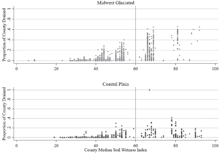
Figure 2 1969 DRAINED ACRES AND SOIL WETNESS INDEX
Notes: Soil wetness index is plotted against 1969 area drained for counties in Midwest states (top panel) and counties in Coastal Plain states (bottom panel). Soil wetness index is the median of 240-meter resolution pixels in each county.
Sources: Authors’ calculations from U.S. Agricultural Census data as digitized by Haines, Fishback, and Rhode (Reference Haines, Fishback and Rhode2015) and the natural soil drainage index from Schaetzl et al. (Reference Schaetzl, Krist, Stanley and Hupy2009).
Empirical Implementation
A difference-in-difference approach to estimating the effects of drainage districts suggests a dynamic panel to compare the effects of district-enabling legislation on wetter counties with those on drier counties—we use a Natural Soil Wetness Index value of 60 to separate the two. For our outcome variables—improved acres in a county, per acre farm value, wheat yields, and corn yields—we estimate the following two-way fixed effects model:
where Y ist is the outcome for county i in state s in year t and PostLaw and HighNSWI are dummies indicating that a state has passed a drainage law and a county is designated as having a high NSWI, respectively. The model includes a county fixed effect, λ i, and three time fixed effects: τ st is a state-by-year fixed effect and ![]() and
and ![]() are group-specific time fixed effects for extremely rough and extremely smooth counties; the latter two sets of coefficients control for treatment effect heterogeneity.Footnote 7
are group-specific time fixed effects for extremely rough and extremely smooth counties; the latter two sets of coefficients control for treatment effect heterogeneity.Footnote 7
The coefficient on PostLaw st × HighNSWI i can be interpreted as the average treatment effect on the treated (ATT) associated with drainage district legislation, provided both wet and dry county outcomes follow parallel trends, and that any shocks affecting the potential outcomes for either group are uncorrelated with treatment. Our comparison group for wet counties is dry counties within the same state. This construction limits threats to identification to those coming from within-state shocks that affect well-drained and poorly drained areas differently, and that occur around the time the state implemented drainage districts.Footnote 8 Comparing high NSWI counties only to others within the same state is important for credible identification because the timing of law passage in each state is affected by that state’s agricultural endowment. Survival plots show the date of drainage district enabling legislation to be heterogeneous across state measures of land productivity, NSWI, and region. Consistent with intuition that selection into legislation occurs first in states able to benefit more from drainage, Kaplan-Meier plots (see Online Appendix Figure A7) show that states in the Midwest, those with higher land productivity, and those with higher natural soil wetness passed legislation earlier.
While contemporaneous accounts provide evidence that it was the drainage districts themselves that enabled naturally wet counties to drain and therefore increase agricultural development and production, our initial empirical approach cannot directly test this assumption because comprehensive data on district formation are not available. Instead, we empirically show that the passage of enabling legislation led to an increase in improved acres and land values. We infer that drainage districts were the enabling middle step. Extending this logic, we subsequently look at within-treatment heterogeneity to understand how coordination problems varied across counties and affected outcomes. We then provide a narrative account of the formation of districts for one state, Illinois, which resulted from enabling legislation intended to do just that.
RESULTS
Land and Value Outcomes
Our data include 13 observations per county, one every 10 years, and we report a window that includes three pre-periods (30 years) and four post-periods (40 years), with period “0” defined as the first year in which treatment in the state begins. A simple before-and-after comparison in our 24-state sample shows that counties with high soil wetness (NSWI>60) saw their improved county acreage increase by 32 percentage points after the passage of drainage district legislation.Footnote 9 Counties with low NSWI also saw increases in improved county acreage between the pre- and post-periods, but the average increase was only 7 percentage points. Consistent with rapid agricultural development over our sample period, both groups of counties saw increasing agricultural land values. Total farm value in low-NSWI counties increased on average from $84M to $267M per county from pre- to post-legislation, while high-NSWI counties saw an average increase from $83M to $397M.
To isolate the effect of drainage district legislation, we implement the difference-in-difference methodology from Equation (1). The main estimates for the effect of drainage on the percentage of a county improved and agricultural land value are presented in Panel A of Table 2. Columns (1) and (2) report the results for all 24 states in our sample. Columns (3)–(6) report separate results for Midwest Glaciated and Coastal Plain states. Column (1) shows that following the implementation of drainage districts, a county with a natural soil wetness index greater than 60 saw a 5.0 percentage point increase in the area of the county with improved agricultural land and a 16.0 percent increase in land value per acre.Footnote 10 The Midwest coefficient estimate is larger than that for the Coastal Plain sample for percentage improved but smaller for the per-acre land value.Footnote 11 The estimates are statistically significant at the 1 percent level or higher and provide evidence that the passage of drainage district legislation was followed by an increase in improved farmland acres and value per acre in counties with naturally wet soils relative to those with lower natural soil wetness.Footnote 12
Table 2 AGRICULTURAL DEVELOPMENT AFTER DRAINAGE DISTRICT LEGISLATION
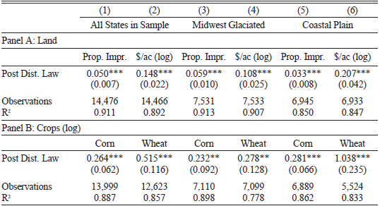
Notes: This table presents difference-in-difference estimates for the effect of drainage district adoption on high NSWI counties relative to others based on the model in Equation (1). Panel A focuses on proportion of county area in improved agricultural land and the log of farmland value per acre. Panel B examines county totals of bushels of wheat and corn (logged). Both panels include state-by-year fixed effects and flexible time controls for counties with roughness higher than the 75th percentile or less than the fifth percentile. Standard errors are clustered by county and reported in parentheses; statistical significance is indicated by *p < 0.1, **p < 0.05, ***p < 0.01.
Sources: Authors’ calculations from U.S. Agricultural Census data as digitized by Haines, Fishback, and Rhode (Reference Haines, Fishback and Rhode2015).
Figure 3 presents the results of an event study using similar county and state-by-year fixed effects while allowing for time-varying treatment effects. The top panel shows coefficient estimates for improved acres, and the bottom for farm value.Footnote 13 All coefficient estimates are normalized relative to a baseline, which is the difference between treated (NSWI> 60) and untreated parcels (NSWI< 60) in the period just prior to treatment. The coefficients for periods t = –2 and t = –3 are the pre-trends. For improved farmland, the t = –3 coefficient is statistically different from 0 at the 5 percent but not at the 1 percent level; other pre-trend coefficients are not different from zero at the 10 percent level. The pre-trend coefficients indicate that the difference-in-difference model estimates are not driven by diverging trends prior to treatment.
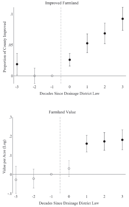
Figure 3 EVENT STUDIES
Notes: The event study model corresponds to the specification in Equation (1) but interacts a flexible time-to-legislation control with NSWI>60 rather than a before/after legislation indicator variable. The specification includes flexible time controls for counties with roughness higher than the 75th percentile or less than the fifth percentile. The difference between counties with NSWI>60 and those with NWSI<60 is normalized to zero in period t = −1, the final period before treatment. Period t = 0 denotes the first period in which a drainage district law exists. The figure pools counties from all 24 states in the sample.
Sources: Authors’ calculations from U.S. Agricultural Census data as digitized by Haines, Fishback, and Rhode (Reference Haines, Fishback and Rhode2015).
From period t = 0 onward in the improved farmland measure and t = 1 onward in the land value measure, there is a statistically significant difference in counties with high NSWI relative to others. The results show that in counties with NSWI>60, improved acreage continued to increase relative to drier counties for four decades, while the capitalization effect is observed by period t = 1 and remains constant thereafter. The improved acreage effect is consistent with implementation taking place over time as districts formed, raised capital, and completed projects. In contrast, the capitalization effect suggests that once a few districts form and are able to operate successfully, the institutional change is capitalized into higher land values and remains relatively static thereafter.
CROP CHOICE
We also apply our empirical strategy to the question of whether drainage, implemented through districts, influenced crop choice. Our sample period spans several eras of agricultural production and market development, and our broad geographic scope encompasses a wide diversity of crops. We examine wheat and corn as key crops where relative advantages might be affected by drainage. Wheat is a versatile crop with winter varieties potentially tolerating several weeks of waterlogging with small yield losses (Cavers and Heard Reference Cavers and Heard2001); corn is a high-value crop with a growing export market throughout our sample period that benefits from the highly fertile soils on drained lands but is more vulnerable to water logging. Today, in the Corn Belt states of Iowa, Illinois, Indiana, Minnesota, and Ohio, 57 percent of corn production occurs in counties with high natural soil wetness. By examining the same regression as specified in Equation (1), but with bushels of wheat or corn as the dependent variable, we can test whether the farmland created by drainage was more favorable to corn production.
The export market for corn expanded from 1850 to 1900 (see Fornari (Reference Fornari1976) for a discussion of U.S. exports of wheat and corn since 1850). Acreage in specific crops is not recorded in the agricultural census until 1880, but bushels of wheat and corn are recorded starting in 1860. From 1860 to 1900, corn production in the 24 states in our sample increased by 238 percent, from 723 million to 2.45 billion bushels. Analysis in this section allows us to causally link drainage district legislation to the increased production of corn in high NSWI counties during this time period.
Coefficient estimates in Panel B of Table 2 suggest a relative increase in corn and wheat production in high NSWI counties over the four decades post drainage district law passage across the entire 24-state sample.Footnote 14 Region-specific results for corn, shown in Columns (3) and (5), reveal similar and statistically significant (at least at the 5 percent level) increases in corn production in both the Coastal Plain and Midwest. Columns (4) and (6) show that the statistical significance of increases in wheat production are similarly statistically significant (at least significant at the 5 percent level), with overall higher coefficient magnitudes driven by Coastal Plain counties. High-NSWI counties in the Coastal Plain produced less than 5,000 bushels of wheat per year prior to drainage district legislation (see Online Appendix Table A5), meaning the actual effect in bushels of wheat is quite small. Conversely, corn production in both the Midwest and Coastal Plain was much larger prior to drainage district legislation. Corn production averaged 579,839 bushels in high-NSWI counties prior to drainage district legislation. The coefficient estimate from (1), (Panel B) shows a 30.2 percent increase (e 0.264−1), or 175,111 bushels of corn, as a result of drainage legislation. Likewise, average wheat production was 121,903 bushels in high NSWI counties prior to legislation and increased by 67.4 percent, or 82,119 bushels, after legislation. In sum, along with evidence of increases in farm values and improved acreage, we find that district coordination led to large increases in corn production, suggesting that the Corn Belt owes its identity, at least in part, to drainage and associated institutional innovation.
TOPOGRAPHY, COORDINATION, AND REGIONAL DIFFERENCES
Our central premise is that drainage districts solve a key coordination challenge, thereby increasing the ability of counties with high natural soil wetness to improve agricultural land via drainage. In the previous section, we demonstrated that the passage of drainage district legislation led to increases in improved agricultural land, land value, and corn and wheat production in counties with naturally wet soils, relative to others. In this section, we use heterogeneity in topography to demonstrate that drainage district legislation benefited those counties best suited to district-scale coordination. Specifically, counties with naturally wet soils and rougher topography, primarily located in the Midwest, do not require drainage districts because there is enough variation in elevation for farmers to drain at least some of their acreage into existing streams directly without coordinating ditches. Similarly, but at the opposite extreme, many Coastal Plain counties are quite flat, and drainage there requires complex coordination beyond the district level, such as state-level legislation to create drainage districts larger than single counties.
In Figure 4, we present a simple theory of the incidence of drainage and the type of coordination employed in its implementation. The theory is consistent with historical narratives and provides predictions about the heterogeneous effects of treatment (the passage of drainage law), which we can test in our empirical analysis. Underlying Figure 4 is the assumption that, once enabled by law, drainage districts are formed where the net benefits relative to alternatives are positive. Furthermore, net benefits to district formation depend on both wetness and ruggedness. Soils with moderate to low natural wetness (west of the vertical axis) are not drained. While Figure 4 is not a map of the United States, it shares some of its features. Most prominently, the areas not benefiting from drainage include large areas west of the 100th meridian, which bisects the Dakotas, Nebraska, Kansas, Oklahoma, and Texas. In the western United States, the problem is not too much water but too little, and farmers supplement natural soil moisture with irrigation (Edwards Reference Edwards2016).

Figure 4 SOIL WETNESS AND TOPOGRAPHY
Source: Authors’ illustration.
For areas wet enough to benefit from drainage, to the right of the vertical axis, the benefits of drainage are increasing in wetness while the costs of coordinating drainage are increasing in flatness. In the most rugged terrain, single-farm drainage entirely avoids coordination costs and can be economical because water is more easily drained into the numerous on-farm streams in rugged landscapes. In flatter terrain, drainage requires coordination with neighbors to address externality and public goods problems. This gives rise to transaction costs, which increase with the geographic scope of the required coordination, and, therefore, with flatness. These features of the technologies of drainage and coordination imply the two rays in Figure 4—frontiers in wetness/roughness space that classify farmland into three categories: acres optimally drained without coordination; acres optimally drained through the coordination of drainage districts; and farmland and potential farmland not drained, despite the potential benefits of drainage, largely due to high coordination costs.
There are historical and empirical counterparts to these three categories. Prior to drainage district authorization, many of the most rugged wet acres, to the northeast in Figure 4, had already been drained. Even after authorization, private drainage avoided the transaction costs of collective action and so remained optimal in some areas. Some farms that were privately drained eventually became incorporated into drainage districts and increased their value through more extensive drainage and connections with off-farm drainage networks.
In the flattest wet areas, to the southeast in Figure 4, drainage required coordination on broad scales. This would have incurred high coordination costs, even under district management, which made the formation of districts uneconomic. Such wet areas, the “swamps of the Yazoo Delta, Mississippi, and those of the eastern part of North Carolina” referred to by Wright (Reference Wright1907), were either never drained or eventually drained through state or federal coordination.
The sweet spot for the drainage district lay between these two extremes: wet areas of intermediate roughness where coordination extended over areas of approximately 100s to 1000s of acres. In such areas, districts dug and maintained ditches and facilitated the connection of individual farms’ drainage networks to those of adjacent farms. Such coordination was made less costly through the powers of eminent domain and taxation granted to drainage districts.
To understand the distribution of topography empirically, we construct a county-level measure of roughness: the standard deviation of 40-meter grid elevation observations in a county. The relationship between roughness and wetness is shown separately for the Midwest and Coastal Plain in the top half of Figure 5. In both regions, wetter counties tend to be flatter. In the Midwest, most wet counties are of mid-range roughness, and none are exceptionally flat (the aforementioned sweet spot). In the Coastal Plain, no wet counties are rough, and many are flat like pancakes. Correlation coefficients between wetness and ruggedness are –0.32 for the Midwest and –0.37 for the Coastal Plain. Notably, the Midwest has 24 counties with NSWI>60 that also exceed the 75th percentile of the overall roughness distribution. These counties are predicted to implement some drainage without the coordination of drainage districts. In the Coastal Plain, the 45 counties that lie at the other extreme—NSWI>60 and in the lowest fifth percentile of the overall roughness distribution—should be less likely to benefit from, and, hence, less likely to form, drainage districts because effective drainage requires coordination over areas too large to manage through drainage districts. These high NSWI and low roughness counties are plotted in Figure 5 and correspond to the lower wedge area in Figure 4, while the high NSWI and very rough counties correspond to the upper wedge area.
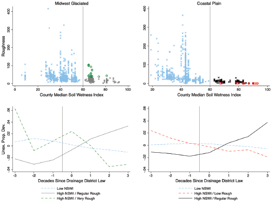
Figure 5 ANALYSIS OF HETEROGENEITY IN ROUGHNESS
Notes: The top panels plot soil wetness index and roughness, defined as the standard deviation of elevation, for counties in the 24 states in our sample. Soil wetness index is the median of 240-meter resolution pixels in each county. High NSWI and very rough counties (24 total) are shown as hollow circles in the top left panel: those with roughness exceeding the 75th percentile with NSWI>60. Counties with low NSWI and very rough topography (45 total) are shown as hollow circles in the top right panel: roughness less than the fifth percentile with NSWI>60. The bottom panels plot the means of the residuals of a regression of proportion of a county in improved agriculture on year and county fixed effects for four mutually exclusive groups.
Sources: Authors’ calculations from U.S. Agricultural Census data as digitized by Haines, Fishback, and Rhode (Reference Haines, Fishback and Rhode2015) and the natural soil drainage index from Schaetzl et al. (Reference Schaetzl, Krist, Stanley and Hupy2009).
In the bottom panels of Figure 5, we plot group means of the residuals of regressions including all counties in our 24 sample states, controlling only for county and state-by-year fixed effects. The left plot contains the mutually exclusive groups of counties in the Midwest with NSWI>60 and regular roughness, those with NSWI>60 and very high roughness, and those with NSWI<60. The right plot shows counties in the Coastal Plain with NSWI>60 and regular roughness, those with NSWI>60 and very low roughness, and those with NSWI<60. In both the Midwest and Coastal Plain, the counties with NSWI<60 serve as placebo subjects—treated with district authorization at the same time, but not expected to benefit from it.
These figures show how topography in the Midwest and the Coastal Plain affect drainage district outcomes. The solid lines in both bottom panels show significant increases in developed agricultural land following the passage of a drainage district law, relative to counties with NSWI below 60. The figures also show that counties with the roughest and smoothest topography do not follow the same treatment trend as other counties with NSWI>60. Accordingly, we modify the regression from Equation (1) by dropping the roughness and smoothness controls and instead allow for three (exclusive) treatment effects in wet NWSI counties after the passage of drainage district legislation: regular roughness, high roughness, and low roughness. Results in Table 5 show baseline effects slightly larger than those in Table 2.Footnote 15 When included separately, both high and low roughness counties exhibit different estimated effects after the passage of legislation: negative, but not statistically significant, coefficients for both topographically rough and smooth counties compared to positive, statistically significant baseline coefficients.Footnote 16 The heterogeneity in treatment effects aligns with the theory of coordination costs depicted in Figure 4 and adds to the evidence that the technology behind agricultural improvement was not solely drainage, but drainage coupled with district coordination.
THE VALUE OF DRAINAGE DISTRICTS
The results in Table 2 provide evidence that the passage of drainage district legislation increased the amount of improved farmland and the per acre value of farmland in counties with high natural soil wetness.Footnote 17 To interpret the economic magnitude of these results, we perform a back-of-the-envelope calculation to estimate the total value of these changes to counties with varying degrees of natural soil wetness. We begin by running a regression similar to the model in Equation (1), but with the treatment variable HighNSWI replaced by bins of natural soil wetness to allow for more heterogeneity in the treatment effect.Footnote 18 The results of running a TWFE model in this manner are shown in Table 4, which provides coefficient estimates relative to a control group of counties with NSWI<50. Examining Columns (2) and (3), the coefficient estimate for the counties with NSWI between 50 and 60 is not statistically different from 0 for value per acre and is slightly negative for proportion improved. For all groups with NSWI>60, the proportion of county improved and value per acre coefficient estimates are positive and significant at the 5 percent level or higher.Footnote 19
To estimate the change in the total land value of a county implied by the estimated treatment effects, assumptions must be made regarding whether the drainage improvements were on the intensive or extensive margin. The value per acre measure is per farm acre, of which improved acres are a subset. Drainage law passage may have induced the draining of new farmland, a change on the extensive margin, or the conversion of existing farmland into the “improved” category, a change on the intensive margin. In reality, we expect that drainage laws affected both margins.
Column (1) of Table 4 shows the same regression run with a different outcome measure: the proportion of total county acres in farmland. These results are not statistically different from zero at the 5 percent level or higher, meaning we are unable to reject the null hypothesis that there was no change on the extensive margin. The point estimates on farmland, however, are similar enough to those on improved acres that we also cannot reject the hypothesis that they are the same, meaning it is possible that the entire increase in improved acres was caused by an extensive adjustment in farmland acres. Because we know a fully extensive or intensive adjustment represent the extremes, we proceed with a dual analysis to bound our value estimates.
Panel A of Table 3 summarizes the characteristics of counties in the sample within each NSWI bin for the observation immediately preceding the passage of drainage laws. We can use the coefficients in Columns (2) and (3) of Table 4 to find the increase in the value of agricultural land in these counties as a result of drainage. Panel B of Table 3 assumes the total amount of farmland remains unchanged, and that all new drainage has occurred on existing farms—an intensification—and so the value of drainage district legislation is calculated by taking the coefficient for each bin (β) from (3) and multiplying e β − 1 by the total acres of farmland. Panel C assumes the other extreme, that total farmland increases by the full amount of the estimated increase in improved acres. This extensive margin effect is found by adding existing improved acres to the product of the coefficient from (2) and total county area. This total area of farmland is then multiplied by e β − 1 to arrive at a per county value increase.
We find that counties with an NSWI between 60 and 70 saw a 14.2–15.1 percent increase in agricultural land value, a narrow range bounded below by the assumption that the estimated land value increases were applicable to the same farmland base as before drainage legislation, and above by adding the estimated increase in improved acres to the total farmland base. The magnitude of the increase in county value for high relative to low NSWI counties is increasing with higher NSWI bins, and we estimate a 14.5–18.1 percent value increase for counties with NSWI between 70 and 80, and a 23.5–27.5 percent increase for counties with NSWI>80. The total increase in farmland in counties with NSWI>60, shown in the first row of Table 3 Panel C, is 81 million acres, about the combined total for improved acres in Illinois, Iowa, and Minnesota in 1910.Footnote 20 Multiplying the per county average land value increase by the number of counties in each bin allows us to arrive at an aggregate intensive margin estimate of $15.7B, while the extensive margin estimate is $17.4B. The increase in land values due to drainage districts was 75 percent of yearly combined crop production around 1910 for the three aforementioned states (Illinois, Iowa, and Minnesota).
Table 3 BACK-OF-ENVELOPE VALUE CALCULATION
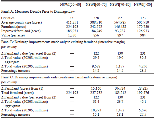
Notes: Panel A provides the number of counties and conditional mean values of four variables. Panel B assumes all drainage improvements are made to existing farmland and estimates for each bin the increase in farmland value per acre using the coefficient estimates from Column (2) in Table 4. This change is multiplied by average county size to get ∆ Total value and then by number of counties to get the aggregate value increase. The percentage increase is relative to total farmland value in the period prior to drainage district legislation passage. Panel C performs the same calculation as Panel B but assumes drainage improvements bring new land into production, and thus uses the coefficient estimates from Column (1) of Table 4 to estimate the change in farmland and Column (2) for the change in per acre value.
Sources: Authors’ calculations from U.S. Agricultural Census data as digitized by Haines, Fishback, and Rhode (Reference Haines, Fishback and Rhode2015).
Table 4 BINNED SOIL WETNESS INDEX RESULTS
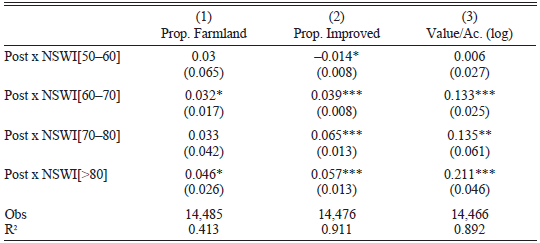
Notes: This table presents difference-in-difference estimates for the effect of drainage district adoption on high drainage index counties relative to others based on the model in Equation (1) but with the treatment variable HighNSWI replaced by bins representing: 50 < NSWI ≤ 60, 60 < NSWI ≤ 70, 70 < NSWI ≤ 80, and 80 ≤ NSWI. Regressions control for county and state-by-year fixed effects and include flexible time controls for those counties with low roughness (standard deviation less than fifth percentile) and high roughness (standard deviation of elevation in the top quartile of all counties). Standard errors are clustered by county and reported in parentheses; statistical significance is indicated by ∗ p < 0.1, ∗∗ p < 0.05, ∗∗∗ p < 0.01.
Sources: Authors’ calculations from U.S. Agricultural Census data as digitized by Haines, Fishback, and Rhode (Reference Haines, Fishback and Rhode2015) and the natural soil drainage index from Schaetzl et al. (Reference Schaetzl, Krist, Stanley and Hupy2009).
Table 5 TREATMENT EFFECT HETEROGENEITY

Notes: This table presents difference-in-difference estimates for the effect of drainage district adoption on high soil wetness index counties (NSWI > 60) relative to others, with counties spilt into three exclusive categories: those with low roughness (standard deviation less than fifth percentile)), high roughness (standard deviation of elevation in the top quartile of all counties); and all remaining counties with NSWI > 60. All specifications include state-by-year and county fixed effects. Standard errors are clustered at the state level and reported in parentheses; statistical significance is indicated by *p < 0.1, **p < 0.05, ***p < 0.01.
Sources: Authors’ calculations from U.S. Agricultural Census data as digitized by Haines, Fishback, and Rhode (Reference Haines, Fishback and Rhode2015).
HOW TECHNOLOGY AND INSTITUTIONS EVOLVED
Our empirical analysis attributes large increases in farmland value to drainage districts and the investments in drainage they induced. We consider here the evolution of the technology and the institutions that led to these effects, as well as the earlier failure of top-down federal and state drainage efforts.
Drain Tile
John Johnston is credited as the Father of Tile Drainage in America. Born in Scotland in 1791, he farmed, married, and emigrated to America at the age of 30. He arrived in New York City in 1821 and purchased 112 acres overlooking Seneca Lake in upstate New York. Around 1835, Johnston began installing underground ceramic drain tiles, manufactured locally using a form that he imported from Scotland. The drained areas saw dramatic increases in yields.
Following Johnston’s innovation came several decades of public debate over the merits of sub-surface drainage—in agricultural society meetings, in writings and speeches by academics, and in popular farming publications such as The Rural New Yorker (see Chamberlain Reference Chamberlain1891). Part of the long period of discussion and adoption had to do with the heterogeneity of soil types and hydrology. Part of it must also have been that the opportunistic draining of farmland was hardly a controlled experiment to assess the merits of a new technology. Furthermore, intrinsically variable yields across farms and crop years made the contribution of drain tile difficult to measure, at least for lands that were not so saturated to begin with that drainage allowed cultivation in the first place.
Ultimately Johnston’s tile idea gained traction. Henry D. French wrote in his book, Farm Drainage: “[n]o system of drainage can be made sufficiently cheap and efficient for general adoption, with other materials than drain tiles” (French Reference French1864). The flat tile method used by Johnston was eventually replaced by cylindrical tile starting around 1858 (McCrory Reference McCrory1928). Local production was dictated by the costs of transporting the heavy tiles, and the first tile manufacturing machine was imported in 1848 from England. Production quickly spread, with 66 tile factories established in the United States from 1850–59, 234 from 1860–69, and 840 from 1870–79 (McCrory Reference McCrory1928).
A caveat to the John Johnston story concerns what he did not contribute. Given the subsequent importance of coordinating drainage schemes, especially in the Midwest, one might expect Johnston and his neighbors to have been wrestling with the same issues: flooding of neighbors’ lands and free-rider problems complicating the construction of ditch networks. We are aware of no such accounts. Article, chapter, and book-length treatments of Johnston’s role in the adoption of subsurface drainage talk exclusively of the back-and-forth debate over the agronomic and economic efficacy of drain tile, and not the external effects or public goods problems arising from transaction costs. A plausible explanation for this dog that did not bark comes from the fact that Seneca County, the home of John Johnston’s farm, is both wet and rugged. Seneca is one of the more than 500 modern counties in the Eastern United States with wet soils (NSWI>60), and among those counties, it ranks in the top 1 percentile for roughness (see Online Appendix Figure A2).
The logic of our empirical analysis of treatment heterogeneity applies here. Seneca’s wetness implies a high value for drainage, and its roughness implies that coordination problems are minimal because areas with greater relief provide more drainage outlets, creeks, and rivers on or near farms. Furthermore, the water drained by Johnston’s tile was easily routed into Seneca Lake, the western boundary of his farm. In other words, the area where John Johnston chose to farm requires drainage, but does not require extensive coordination among neighbors. Johnston and others were incentivized to drain and tinker with drain tile without having to simultaneously solve the coordination problems that initially blocked widespread drainage in the flatter wet counties, notably those in the Midwest.
One might ask if Johnston’s decision to farm in a wet and rugged area reflected great foresight that his innovation to come would be lower cost absent the coordination problems posed in flatter wet areas. Or possibly he chose to settle where he did because the terrain was similar to the Scottish Southern Uplands where he grew up. Or possibly there were 50 other John Johnstons who settled in wet, but flatter, parts of the Eastern United States in the 1830s, each experimenting with drainage methods but stymied by the requirement that they solve both technological puzzles and a wholly different set of collective action problems. We do not know which, if any, of these conjectures explain Johnston’s central role in the history of drainage. We do know that Seneca County, the Cradle of Drainage in America, is almost uniquely wet and rugged.
Federal and State Wetland Policies
Roughly coincident with the development of drain tile were federal efforts to address wetlands in the federal domain that were “unproductive and an economic waste” (Palmer Reference Palmer1915). To encourage development and drainage, Congress allocated substantial swampland to the states through a series of Swamp Land Acts (1849, 1850, and 1860). The lands made available to the states under the Acts are shown in Online Appendix Table A10. The first of the Acts granted 9.5 million acres of federal land to Louisiana—28 percent of its combined land and water area. The clear federal impetus for the legislation was to regulate the annual spring flooding of the Mississippi River. There was also substantial support in the state for draining swamplands that lay more permanently underwater.
After passage of the 1849 Act, the Louisiana legislature divided the state into districts and established a statewide board that sold swampland in each district, prioritized drainage projects, and put selected projects out for bid. The highest-priority projects invariably were repairing and constructing levees to protect farmland in the Southern Mississippi River Alluvial Valley. The Louisiana system may seem unexceptional from a twenty-first-century perspective, but Vileisis (Reference Vileisis1997, p. 79) notes that “at the time such division of lands and establishment of additional governance was revolutionary,” requiring “citizens to accept a whole new vision of the proper role of state government.”
The first Swampland Act in 1849 was followed in 1850 by similar legislation granting over 50 million acres to 12 widely scattered states, and a third Act in 1860 for two more states. In each case, states were left to devise their own means of drainage and improvement, and their methods varied. Even neighboring states differed in their approaches. While Indiana managed the drainage of its 1.3 million acres at the state level, Illinois distributed its 1.5 million acres directly to counties.
Ultimately, the Swampland Acts were unsuccessful in taming the Mississippi—both initially and following the disruption of the Civil War—and unsuccessful in inducing much drainage.Footnote 21 Despite this failure, the methods employed by the state to dispose of and manage lands would prove to be important forerunners of the ultimately more successful institutional innovation of drainage districts.
Institutional Evolution Leading to Drainage Districts—A Case Study of Illinois
While drainage technology was developed and debated roughly between 1835 and 1865, the body of law that codified drainage districts and their ditch law equivalents (see Ohio) developed mainly later, between 1855 and 1912. Relatively early in this process, and early in terms of its own settlement, was the Illinois drainage district law passed in 1879. The legal evolution prior to the 1879 law in the state that became the leading corn producer for much of the twentieth century provides a case study of the coordination problems that inhibited drainage investment prior to drainage districts.
TWO DRAINAGE PROBLEMS AND TWO TYPES OF DISTRICTS
The earliest settlement in Illinois occurred along the Wabash, Ohio, and Mississippi rivers—the western and southeastern borders of the state, created in 1818. Excellent flood plain soil was available to be tilled once the bottom lands were cleared of timber. Prairie land, away from the rivers, initially held little interest due to the difficulty in breaking prairie sod and the often-flooded soils (Illinois Tax Commission 1941, p. 2). The difficulties of sod busting were significantly reduced by the invention and mass production of the self-scouring steel plow in the 1830s, usually credited to John Deere, an Illinois blacksmith. With the technical means to cultivate more easily, and as the bottom lands filled with settlers, attention turned to prairie lands and the challenges of drainage. Managing excess water on agricultural lands in Illinois and elsewhere in the Midwest posed two problems: “sub-soil drainage and open ditches in some parts of the state and flood and high-water protection in others” (Illinois Tax Commission 1941, p. 2). Just as there are two drainage problems, Illinois law since 1879 has recognized two closely related types of drainage districts: levee districts and tile-and-ditch districts.
Levee districts addressed the challenges of protecting river bottoms from floods. They constructed protective levees along rivers and open ditches to carry water from inland areas denied their usual outlet to the river by the levees. Because much of the land protected by levees sits near river level, modern levee districts operate pumping plants to keep groundwater levels low enough for farming (see, e.g., Board of Commissioners of the Sny Island Levee Drainage District 2022).
Tile and open ditch districts were organized to drain open prairie land. Leaving the installation of tile to individual landowners, tile-and-ditch districts typically build outlet ditches used in common by multiple landowners and coordinate the interconnection of private drain tile systems. Tile-and-ditch districts are initially capital intensive when ditches are dug and eminent domain is exercised. Most become inactive after ditch construction.
While the two types of districts are treated very similarly under Illinois law, and both types were authorized in the same year, the evolution of Illinois drainage law that led to their creation in 1879 seems mainly to have been driven by flood control.
DRAINAGE BEFORE DISTRICT AUTHORIZATION IN 1879
Various legal means were used to effect drainage and flood control before districts were authorized in Illinois in 1879. Two were important forerunners to modern drainage districts: action under common law and legislatively-created charter companies.
As to common law, drainage rights lay in the public domain before the potential value of farm drainage and flood protection warranted their invention and allocation. As land and rights to drain became more valuable, two alternative common law rules were adopted by different states. Illinois, unlike Indiana, Minnesota, and Missouri, adopted a “dominant heritage” rule, granting rights of drainage to upstream property owners. While this rule would seem to break the Coasean logjam by a clear definition of rights, it turned out to be insufficient. The dominant heritage rule insisted that upstream landowners could drain water onto downstream neighbors only through “natural” channels. The right to build new ditches and drain into them, or to block such drainage, remained unsettled.
The second challenge difficult to address through common law was that of organizing collective action (Illinois Tax Commission 1941, p. 41). In the early and mid-nineteenth century, common law drainage rights were supplemented under the first two Illinois state constitutions (of 1818 and 1848) by granting the legislature authority to issue charters to private parties. Powers granted to charters were various and foreshadowed those ultimately held by districts. In attempts to induce drainage and flood protection, chartered companies were given lands, money, and taxing authority, and sometimes claims to future property tax revenue (Illinois Tax Commission 1941, p. 41). While charter companies achieved some success in getting levees built and ditches dug, an 1869 Illinois Supreme Court opinion held that they violated the state constitution on the grounds of taxing residents and supposed drainage beneficiaries without their political representation.
The definitive district-authorizing law comprised two bills, the Drainage and Levee Act and the Farm Drainage Act, which were passed by the Illinois legislature in 1879, 60 years after the first legislative authorization of a charter company. Before their passage, a prototype act authorizing districts was passed in 1871 at the urging of levee interests in the Sny Island area. However, in 1876, districts under this legislation, like charter companies before them, were found to be constitutionally defective. The situation was remedied by an amendment to the Illinois Constitution in 1878, followed the next year by the two district authorization acts.
DRAINAGE DISTRICT FORMATION AFTER 1879
In earlier sections, we measured the effects on drainage and farm value made possible, state by state, by the authorization of drainage districts. In every state, those outcomes coincided with the decades-long process of creating drainage districts and carrying out their investment plans. In Illinois, this process is reflected in the top panel of Figure 6, based on data from a 1941 Illinois Tax Commission monograph displaying acreage in districts created as a result of the 1879 district authorization (see Online Appendix Table A11 for number of districts as well as acreage).

Figure 6 ILLINOIS DRAINAGE DISTRICTS
Notes: The top panel shows the area in drainage districts over time. The bottom panel shows the results of an event study corresponding to the specification in Equation (1) but interacting a flexible time to legislation control with NSWI>60 rather than a before/after legislation indicator variable and using counties solely from Illinois. The specification includes flexible time controls for counties with roughness higher than the 75th percentile. The difference between counties with NSWI>60 and those with NWSI<60 is normalized to zero in 1870, the final period before legislation passage.
Sources: Data in top panel is from Illinois Tax Commission (1941). Data in bottom panel is from U.S. Agricultural Census as digitized by Haines, Fishback, and Rhode (Reference Haines, Fishback and Rhode2015).
The bottom panel of Figure 6 shows the corresponding event study constructed, as are our aggregate results shown in Figure 3, but estimated over a panel of only Illinois counties. A comparison of the two demonstrates broad agreement between our empirical estimate of the effects of drainage district legislation and the data on acres in districts in Illinois (for which we lack data in other states). The top panel shows the total acres in districts for all counties in Illinois, which should largely represent drained acres in high NSWI counties, but will include some undrained areas and acres in low-NSWI counties. The bottom panel estimates the relative effect on improved acreage of being in a high-NSWI county in Illinois relative to the last pre-district observation, 1870, in a low-NSWI county. While we do not observe drained acres directly, we infer that in high-NSWI counties, many of the new acres are attributable to drainage. Prior to 1870, increases in improved acreage in high-NSWI counties occurred due to development without drainage and drainage development absent districts. The period of experimentation with drainage prior to drainage districts is seen in the uptick in coefficient estimates from 1860 to 1870.
CONCLUSION
In this paper, we study the historical record of farm drainage in the eastern half of the United States and estimate the role played by coordinating governance institutions. After the failure of federal and state actions to stimulate drainage in the mid-nineteenth century, locally initiated drainage districts spurred investment over millions of acres. States in our sample adopted district-enabling drainage laws between 1859 and 1912, and after adoption, we find in each state substantial increases in improved agricultural land and land values, comparing counties with naturally wet soils to those with lower soil wetness. Because the choice to pass legislation was endogenously determined, one should be cautious in extrapolating our coefficient estimates to predict the effects of district legislation in other places and times. For instance, had North Carolina passed its enabling legislation in 1879 when Illinois did, we would expect it to have resulted in smaller gains than either Illinois’ passage that year or North Carolina’s eventual passage in 1909.
Although environmental effects of the large-scale conversion of wetlands to agricultural lands were not considered when drainage was implemented (or did not receive much consideration due to the local focus of drainage districts), drainage has resulted in habitat destruction, loss of flood control, and degraded water quality (Edwards and Thurman Reference Edwards, Thurman, Gary and Dinar2024). Our direct extensive margin estimate suggests that in counties with median NSWI>60, a maximum conversion directly from wetlands to farmland of just under 11 million acres occurred as a result of drainage district legislation.Footnote 22
Today, the Corn Belt states—Minnesota, Iowa, Indiana, Illinois, and Ohio—produce over 50 percent of their corn in counties with high natural soil wetness. In the United States more broadly, naturally wet counties in our sample account for 19 percent of agricultural land value and produce 38 percent of corn value. We estimate that district-induced drainage increased the value of agricultural land in these counties by 20–37 percent, or $16.8–18.7 billion in 2020 dollars.


 Open access