


1. Introduction
In turbulence there is little question that an energy cascade exists, whereby energy injected at the largest scales of a flow is eventually dissipated to heat by viscosity. However, there is still much to debate as to how this cascade works – the relevant mechanisms and flow structures, the validity of the so called ‘Richardson’ cascade and the degree of time and space locality in the cascade – are all open questions (Tsinober Reference Tsinober2009; Vela-Martín & Jiménez Reference Vela-Martín and Jiménez2021; Johnson & Wilczek Reference Johnson and Wilczek2024).

Figure 1. (a) Schematic of typical
 $\boldsymbol{\omega }$
-
$\boldsymbol{\omega }$
-
 $\unicode{x1D64E}$
alignment. Here,
$\unicode{x1D64E}$
alignment. Here,
 $\boldsymbol{\omega }$
is indicated by the yellow line and swirl. The baseline/universal preference for alignment between
$\boldsymbol{\omega }$
is indicated by the yellow line and swirl. The baseline/universal preference for alignment between
 $\boldsymbol{\omega }$
and
$\boldsymbol{\omega }$
and
 $\boldsymbol{e}_2 \,$
is shown. To maximise vortex stretching,
$\boldsymbol{e}_2 \,$
is shown. To maximise vortex stretching,
 $\boldsymbol{\omega }$
(yellow line) would be aligned more with
$\boldsymbol{\omega }$
(yellow line) would be aligned more with
 $\boldsymbol{e}_1 \,$
, which has been found generally to not be the case in turbulence. (b) Schematic illustrating strain-rate self-amplification (SSA) in a one- and three-dimensional sense. In one dimension, an initial compressive strain (red line) causes the opposing velocities to steepen the negative gradient of the curves as time progresses, which in turn increases the compressive strain, until a singularity/shock forms (black line) as in the Burgers one-dimensional equation. The same idea is illustrated in three dimensions, where an initially cylindrical fluid parcel (or vortex) is compressed along one axis, and stretched in two others, in turn increasing the compressive strain.
$\boldsymbol{e}_1 \,$
, which has been found generally to not be the case in turbulence. (b) Schematic illustrating strain-rate self-amplification (SSA) in a one- and three-dimensional sense. In one dimension, an initial compressive strain (red line) causes the opposing velocities to steepen the negative gradient of the curves as time progresses, which in turn increases the compressive strain, until a singularity/shock forms (black line) as in the Burgers one-dimensional equation. The same idea is illustrated in three dimensions, where an initially cylindrical fluid parcel (or vortex) is compressed along one axis, and stretched in two others, in turn increasing the compressive strain.
Perhaps motivated by Richardson’s ‘whirl’ centric poetic verse, a large portion of previous works focus on probing the cascade primarily through the characterisation of the vorticity vector,
 $\boldsymbol{\omega }$
, and secondly via the strain-rate tensor,
$\boldsymbol{\omega }$
, and secondly via the strain-rate tensor,
 $\unicode{x1D64E}$
, which is simply the symmetric portion of the velocity-gradient tensor,
$\unicode{x1D64E}$
, which is simply the symmetric portion of the velocity-gradient tensor,
 $\unicode{x1D63C} \; = \nabla \boldsymbol{u} = \partial u_i / \partial x_j$
,
$\unicode{x1D63C} \; = \nabla \boldsymbol{u} = \partial u_i / \partial x_j$
,
 $u$
is the velocity field. Much of the literature has focused on the alignment and interaction of
$u$
is the velocity field. Much of the literature has focused on the alignment and interaction of
 $\omega _i = \epsilon _{ijk} \partial {u_k} / \partial {x_j}$
and the eigenvectors of
$\omega _i = \epsilon _{ijk} \partial {u_k} / \partial {x_j}$
and the eigenvectors of
 $\, S_{ij} =( {1}/{2}) (\partial u_i / \partial x_j + \partial u_j / \partial x_i)$
(as in figure 1
a), as they are thought to be the primary cause of nonlinearity in the vorticity dynamics (Hamlington, Schumacher & Dahm Reference Hamlington, Schumacher and Dahm2008). As such, there has been an effort to link the energy cascade with the geometry of
$\, S_{ij} =( {1}/{2}) (\partial u_i / \partial x_j + \partial u_j / \partial x_i)$
(as in figure 1
a), as they are thought to be the primary cause of nonlinearity in the vorticity dynamics (Hamlington, Schumacher & Dahm Reference Hamlington, Schumacher and Dahm2008). As such, there has been an effort to link the energy cascade with the geometry of
 $\unicode{x1D63C}$
, particularly as it is implicitly assumed in many sub-grid-scale turbulence models that the velocity gradient at resolved (large) scales can be used to determine energy transfer at the unresolved (small) scales (Smagorinsky Reference Smagorinsky1963; Vela-Martín & Jiménez Reference Vela-Martín and Jiménez2021). We point the reader to the excellent recent review by Johnson & Wilczek (Reference Johnson and Wilczek2024) for a more nuanced discussion of the current research, but we will highlight some of the more pertinent works here.
$\unicode{x1D63C}$
, particularly as it is implicitly assumed in many sub-grid-scale turbulence models that the velocity gradient at resolved (large) scales can be used to determine energy transfer at the unresolved (small) scales (Smagorinsky Reference Smagorinsky1963; Vela-Martín & Jiménez Reference Vela-Martín and Jiménez2021). We point the reader to the excellent recent review by Johnson & Wilczek (Reference Johnson and Wilczek2024) for a more nuanced discussion of the current research, but we will highlight some of the more pertinent works here.
The eigenvectors of
 $\unicode{x1D64E}$
define its principal axes, which are also the directions of extremal strain. They are defined as
$\unicode{x1D64E}$
define its principal axes, which are also the directions of extremal strain. They are defined as
 $\boldsymbol{e}_1 \,$
,
$\boldsymbol{e}_1 \,$
,
 $\boldsymbol{e}_2 \,$
,
$\boldsymbol{e}_2 \,$
,
 $\boldsymbol{e}_3 \,$
, where
$\boldsymbol{e}_3 \,$
, where
 $\boldsymbol{e}_1 \,$
and
$\boldsymbol{e}_1 \,$
and
 $\boldsymbol{e}_3 \,$
are always the most extensive and compressive vectors, respectively. Conversely, for incompressible flows
$\boldsymbol{e}_3 \,$
are always the most extensive and compressive vectors, respectively. Conversely, for incompressible flows
 $\boldsymbol{e}_2 \,$
can either be extensive or compressive depending on the local flow. One of the most consistent, but perhaps counterintuitive, findings in this field has been that
$\boldsymbol{e}_2 \,$
can either be extensive or compressive depending on the local flow. One of the most consistent, but perhaps counterintuitive, findings in this field has been that
 $\boldsymbol{\omega }$
has a prevalence to align with
$\boldsymbol{\omega }$
has a prevalence to align with
 $\boldsymbol{e}_2 \,$
(also shown to be predominately extensive), and not
$\boldsymbol{e}_2 \,$
(also shown to be predominately extensive), and not
 $\boldsymbol{e}_1$
, which would result in the maximal amount of vortex stretching (Betchov Reference Betchov1956; Ashurst et al. Reference Ashurst, Kerstein, Kerr and Gibson1987; Tsinober & Kit Reference Tsinober and Kit1992; Hamlington et al. Reference Hamlington, Schumacher and Dahm2008; Buaria, Bodenschatz & Pumir Reference Buaria, Bodenschatz and Pumir2020). These same works have also reported the more slight preference for
$\boldsymbol{e}_1$
, which would result in the maximal amount of vortex stretching (Betchov Reference Betchov1956; Ashurst et al. Reference Ashurst, Kerstein, Kerr and Gibson1987; Tsinober & Kit Reference Tsinober and Kit1992; Hamlington et al. Reference Hamlington, Schumacher and Dahm2008; Buaria, Bodenschatz & Pumir Reference Buaria, Bodenschatz and Pumir2020). These same works have also reported the more slight preference for
 $\boldsymbol{\omega }$
to orient itself perpendicular to the most compressive strain axis,
$\boldsymbol{\omega }$
to orient itself perpendicular to the most compressive strain axis,
 $\boldsymbol{e}_3 \,$
. An illustration of this preferred alignment is shown in figure 1(a). The prevalence of these findings across theory, direct numerical simulations (DNS), experiments and a range of turbulent flows lend credence to the idea that these vortex alignment preferences may be considered a universal feature of turbulent flows.
$\boldsymbol{e}_3 \,$
. An illustration of this preferred alignment is shown in figure 1(a). The prevalence of these findings across theory, direct numerical simulations (DNS), experiments and a range of turbulent flows lend credence to the idea that these vortex alignment preferences may be considered a universal feature of turbulent flows.
Despite the predominance of
 $\boldsymbol{\omega }$
alignment with
$\boldsymbol{\omega }$
alignment with
 $\boldsymbol{e}_2 \,$
, other works provide arguments as to why it is nevertheless the alignment of
$\boldsymbol{e}_2 \,$
, other works provide arguments as to why it is nevertheless the alignment of
 $\boldsymbol{\omega }$
and
$\boldsymbol{\omega }$
and
 $\boldsymbol{e}_1 \,$
that is the main driver of enstrophy generation and energy cascade (Hamlington et al. Reference Hamlington, Schumacher and Dahm2008; Buxton & Ganapathisubramani Reference Buxton and Ganapathisubramani2010; Buaria & Pumir Reference Buaria and Pumir2021). Looking at the individual contributions of each strain-rate eigenvector to enstrophy production, some found the contribution from
$\boldsymbol{e}_1 \,$
that is the main driver of enstrophy generation and energy cascade (Hamlington et al. Reference Hamlington, Schumacher and Dahm2008; Buxton & Ganapathisubramani Reference Buxton and Ganapathisubramani2010; Buaria & Pumir Reference Buaria and Pumir2021). Looking at the individual contributions of each strain-rate eigenvector to enstrophy production, some found the contribution from
 $\boldsymbol{e}_1 \,$
to be slightly larger than that of
$\boldsymbol{e}_1 \,$
to be slightly larger than that of
 $\boldsymbol{e}_2 \,$
, with a difference that increased with Reynolds number,
$\boldsymbol{e}_2 \,$
, with a difference that increased with Reynolds number,
 $Re$
(Jimenez et al. Reference Jiménez, Wray, Saffman and Rogallo1993; Buaria et al. Reference Buaria, Pumir, Bodenschatz and Yeung2019; Zhou & Frank Reference Zhou and Frank2021). Hamlington et al. (Reference Hamlington, Schumacher and Dahm2008) and Buaria & Pumir (Reference Buaria and Pumir2021) showed that the
$Re$
(Jimenez et al. Reference Jiménez, Wray, Saffman and Rogallo1993; Buaria et al. Reference Buaria, Pumir, Bodenschatz and Yeung2019; Zhou & Frank Reference Zhou and Frank2021). Hamlington et al. (Reference Hamlington, Schumacher and Dahm2008) and Buaria & Pumir (Reference Buaria and Pumir2021) showed that the
 $\boldsymbol{\omega }$
–
$\boldsymbol{\omega }$
–
 $\boldsymbol{e}_1 \,$
alignment was achieved after removing the local, self-induced, strain rate, while Xu, Pumir & Bodenschatz (Reference Xu, Pumir and Bodenschatz2011) showed that this alignment occurred at some characteristic lag time. Other authors use the joint probability distribution of the second and third velocity-gradient invariants. Q is the 2nd invariant, R the 3rd invariant ( a ‘QR plot’) to demonstrate the prevalence of vortex stretching over vortex compression. Buxton & Ganapathisubramani (Reference Buxton and Ganapathisubramani2010) combined both approaches and found the
$\boldsymbol{e}_1 \,$
alignment was achieved after removing the local, self-induced, strain rate, while Xu, Pumir & Bodenschatz (Reference Xu, Pumir and Bodenschatz2011) showed that this alignment occurred at some characteristic lag time. Other authors use the joint probability distribution of the second and third velocity-gradient invariants. Q is the 2nd invariant, R the 3rd invariant ( a ‘QR plot’) to demonstrate the prevalence of vortex stretching over vortex compression. Buxton & Ganapathisubramani (Reference Buxton and Ganapathisubramani2010) combined both approaches and found the
 $\boldsymbol{\omega }$
-
$\boldsymbol{\omega }$
-
 $\unicode{x1D64E}$
alignment for each region of QR space. While the alignment behaviour of
$\unicode{x1D64E}$
alignment for each region of QR space. While the alignment behaviour of
 $\boldsymbol{e}_2 \,$
stayed the same throughout, areas with
$\boldsymbol{e}_2 \,$
stayed the same throughout, areas with
 $R \lt 0$
displayed
$R \lt 0$
displayed
 $\boldsymbol{\omega }$
-
$\boldsymbol{\omega }$
-
 $\boldsymbol{e}_1 \,$
alignment. Thereby they argued that the extensive
$\boldsymbol{e}_1 \,$
alignment. Thereby they argued that the extensive
 $\boldsymbol{e}_1 \,$
alignment is more important for determining enstrophy production or destruction, and that the universally flat distribution of
$\boldsymbol{e}_1 \,$
alignment is more important for determining enstrophy production or destruction, and that the universally flat distribution of
 $\boldsymbol{e}_1 \,$
alignment in other works is due to the summation of the different behaviours throughout QR space.
$\boldsymbol{e}_1 \,$
alignment in other works is due to the summation of the different behaviours throughout QR space.
On the other hand, many other works propose that the alignment of
 $\boldsymbol{\omega }$
and
$\boldsymbol{\omega }$
and
 $\unicode{x1D64E}$
is over-emphasised and instead the self-amplification of strain rate is most important (Vincent & Meneguzzi Reference Vincent and Meneguzzi1994; Tsinober Reference Tsinober1998, Reference Tsinober2009; Carbone & Bragg Reference Carbone and Bragg2020; Johnson Reference Johnson2020, Reference Johnson2021; Vela-Martín & Jiménez Reference Vela-Martín and Jiménez2021). For instance Vincent & Meneguzzi (Reference Vincent and Meneguzzi1994) presented evidence that enstrophy production is actually driven largely by the shear instability of vortex sheets. Similarly Tsinober (Reference Tsinober2009) showed the cascade is caused more via the compression of fluid elements and strain self-amplification than by vortex stretching. A key to these arguments is the non-local nature of
$\unicode{x1D64E}$
is over-emphasised and instead the self-amplification of strain rate is most important (Vincent & Meneguzzi Reference Vincent and Meneguzzi1994; Tsinober Reference Tsinober1998, Reference Tsinober2009; Carbone & Bragg Reference Carbone and Bragg2020; Johnson Reference Johnson2020, Reference Johnson2021; Vela-Martín & Jiménez Reference Vela-Martín and Jiménez2021). For instance Vincent & Meneguzzi (Reference Vincent and Meneguzzi1994) presented evidence that enstrophy production is actually driven largely by the shear instability of vortex sheets. Similarly Tsinober (Reference Tsinober2009) showed the cascade is caused more via the compression of fluid elements and strain self-amplification than by vortex stretching. A key to these arguments is the non-local nature of
 $\boldsymbol{\omega }$
-
$\boldsymbol{\omega }$
-
 $\unicode{x1D64E}$
interactions, the direct relationship between strain and energy dissipation and the highly nonlinear nature of strain-dominated regions (Tsinober Reference Tsinober1998, Reference Tsinober2009). Several related works used the QR space to claim that most nonlinear flow behaviour occurs in areas with high strain production, while nonlinearity is relatively repressed in regions of high vorticity (Tsinober Reference Tsinober1998; Gulitski et al. Reference Gulitski, Kholmyansky, Kinzelbach, Lüthi, Tsinober and Yorish2007; Tsinober Reference Tsinober2009). Further, while strain production has been found to only depend on strain, vortex stretching has been shown to actually deplete strain production (Betchov Reference Betchov1956; Tsinober Reference Tsinober2009). Interestingly, Donzis, Yeung & Sreenivasan (Reference Donzis, Yeung and Sreenivasan2008) and Buaria et al. (Reference Buaria, Pumir, Bodenschatz and Yeung2019) also found that, while extreme strain events were co-located with equally large enstrophy events, intense vorticity events were accompanied by relatively less strain. The fact that enstrophy and strain share the same mean value, yet enstrophy appears more intermittent, is thought to be due to the fact that vortex stretching amplifies vorticity while depleting strain (Ishihara, Gotoh & Kaneda Reference Ishihara, Gotoh and Kaneda2009; Buaria et al. Reference Buaria, Pumir, Bodenschatz and Yeung2019).
$\unicode{x1D64E}$
interactions, the direct relationship between strain and energy dissipation and the highly nonlinear nature of strain-dominated regions (Tsinober Reference Tsinober1998, Reference Tsinober2009). Several related works used the QR space to claim that most nonlinear flow behaviour occurs in areas with high strain production, while nonlinearity is relatively repressed in regions of high vorticity (Tsinober Reference Tsinober1998; Gulitski et al. Reference Gulitski, Kholmyansky, Kinzelbach, Lüthi, Tsinober and Yorish2007; Tsinober Reference Tsinober2009). Further, while strain production has been found to only depend on strain, vortex stretching has been shown to actually deplete strain production (Betchov Reference Betchov1956; Tsinober Reference Tsinober2009). Interestingly, Donzis, Yeung & Sreenivasan (Reference Donzis, Yeung and Sreenivasan2008) and Buaria et al. (Reference Buaria, Pumir, Bodenschatz and Yeung2019) also found that, while extreme strain events were co-located with equally large enstrophy events, intense vorticity events were accompanied by relatively less strain. The fact that enstrophy and strain share the same mean value, yet enstrophy appears more intermittent, is thought to be due to the fact that vortex stretching amplifies vorticity while depleting strain (Ishihara, Gotoh & Kaneda Reference Ishihara, Gotoh and Kaneda2009; Buaria et al. Reference Buaria, Pumir, Bodenschatz and Yeung2019).
The behaviour of the velocity gradient during ‘extreme events’ in the energy cascade is also of much interest. The link between
 $\unicode{x1D63C}$
morphology and extreme energy transfer events can be easily made by considering that, in the one-dimensional (1-D) Burgers equation, strain self-amplification is responsible for singularity and shock formation in the inviscid limit (Johnson & Wilczek Reference Johnson and Wilczek2024). This idea was extended to three dimensions with the so-called ‘restricted Euler’ equation, which has been shown to produce finite time singularities in the absence of the anisotropic pressure Hessian and viscosity (Vieillefosse Reference Vieillefosse1982, Reference Vieillefosse1984). Notably, the morphologies which ought to bring about this singularity are those found ubiquitously in turbulent flows: two extensional strain directions (
$\unicode{x1D63C}$
morphology and extreme energy transfer events can be easily made by considering that, in the one-dimensional (1-D) Burgers equation, strain self-amplification is responsible for singularity and shock formation in the inviscid limit (Johnson & Wilczek Reference Johnson and Wilczek2024). This idea was extended to three dimensions with the so-called ‘restricted Euler’ equation, which has been shown to produce finite time singularities in the absence of the anisotropic pressure Hessian and viscosity (Vieillefosse Reference Vieillefosse1982, Reference Vieillefosse1984). Notably, the morphologies which ought to bring about this singularity are those found ubiquitously in turbulent flows: two extensional strain directions (
 $\boldsymbol{e}_1$
,
$\boldsymbol{e}_1$
,
 $\boldsymbol{e}_2 $
) and preferential
$\boldsymbol{e}_2 $
) and preferential
 $\boldsymbol{\omega }$
-
$\boldsymbol{\omega }$
-
 $\boldsymbol{e}_2 \,$
alignment, i.e. figure 1(a). Strain self-amplification (illustrated in figure 1
b) occurs strictly due to the positivity of
$\boldsymbol{e}_2 \,$
alignment, i.e. figure 1(a). Strain self-amplification (illustrated in figure 1
b) occurs strictly due to the positivity of
 $\boldsymbol{e}_2 \,$
, and it is predicted that the singularity will occur along the region in QR space affiliated with that straining mechanism (Vieillefosse Reference Vieillefosse1982, Reference Vieillefosse1984; Johnson Reference Johnson2021; Johnson & Wilczek Reference Johnson and Wilczek2024). These ideas have been supported by other works investigating extreme events in enstrophy, which have simultaneously found enhanced
$\boldsymbol{e}_2 \,$
, and it is predicted that the singularity will occur along the region in QR space affiliated with that straining mechanism (Vieillefosse Reference Vieillefosse1982, Reference Vieillefosse1984; Johnson Reference Johnson2021; Johnson & Wilczek Reference Johnson and Wilczek2024). These ideas have been supported by other works investigating extreme events in enstrophy, which have simultaneously found enhanced
 $\boldsymbol{\omega }$
-
$\boldsymbol{\omega }$
-
 $\boldsymbol{e}_2 \,$
alignment, and a quasi-2-D structure during the event (Jimenez et al. Reference Jiménez, Wray, Saffman and Rogallo1993; Buaria et al. Reference Buaria, Pumir, Bodenschatz and Yeung2019, Reference Buaria, Bodenschatz and Pumir2020; Zhou & Frank Reference Zhou and Frank2021). Finally, Vela-Martín & Jiménez (Reference Vela-Martín and Jiménez2021) investigated the morphological and probabilistic differences between downscale and upscale energy transfers. They found these to be mainly driven by strain-dominated energy fluxes, where downscale transfer was most correlated with strain-dominated regions. Additional investigation of the velocity-gradient structure for upscale energy transfer showed that, while vortex stretching and compression exist in both cascade directions (albeit in different proportions), strain-dominated regions depend strongly on the cascade direction.
$\boldsymbol{e}_2 \,$
alignment, and a quasi-2-D structure during the event (Jimenez et al. Reference Jiménez, Wray, Saffman and Rogallo1993; Buaria et al. Reference Buaria, Pumir, Bodenschatz and Yeung2019, Reference Buaria, Bodenschatz and Pumir2020; Zhou & Frank Reference Zhou and Frank2021). Finally, Vela-Martín & Jiménez (Reference Vela-Martín and Jiménez2021) investigated the morphological and probabilistic differences between downscale and upscale energy transfers. They found these to be mainly driven by strain-dominated energy fluxes, where downscale transfer was most correlated with strain-dominated regions. Additional investigation of the velocity-gradient structure for upscale energy transfer showed that, while vortex stretching and compression exist in both cascade directions (albeit in different proportions), strain-dominated regions depend strongly on the cascade direction.
In this work we will combine approaches used in previous works to address several unanswered questions. Of main interest is how the morphology of the velocity gradient behaves for the largest upscale and downscale energy transfer events. We will condition morphological statistics on the energy transfer amplitude and make use of both the QR and
 $\boldsymbol{\omega }$
-
$\boldsymbol{\omega }$
-
 $\unicode{x1D64E}$
alignment methods to probe the behaviour. In the next sections we introduce our experimental facility (§ 2) and the main quantities of interest (§ 3), and then display non-conditioned morphological statistics (§ 4.1). We then provide the conditioned statistics in § 4.2 and finish by discussing their implications from different perspectives in § 5.
$\unicode{x1D64E}$
alignment methods to probe the behaviour. In the next sections we introduce our experimental facility (§ 2) and the main quantities of interest (§ 3), and then display non-conditioned morphological statistics (§ 4.1). We then provide the conditioned statistics in § 4.2 and finish by discussing their implications from different perspectives in § 5.
2. Experimental giant von Kármán facility
The data presented in this work are purely experimental and are collected from the giant von Kármán (GvK) facility at CEA Paris-Saclay. This state of the art facility has been described extensively in previous works, so we resort to a quick summary here (Cheminet et al. Reference Cheminet, Ostovan, Valori, Cuvier, Daviaud, Debue, Dubrulle, Foucaut and Laval2021; Debue et al. Reference Debue, Valori, Cuvier, Daviaud, Foucaut, Laval, Wiertel, Padilla and Dubrulle2021, Dubrulle et al. Reference Dubrulle, Daviaud, Faranda, Marié and Saint-Michel2022). The facility (figure 2
a) consists of a large cylindrical tank with radius (
 $r$
) and height (distance between impellers) of 0.5 and 0.9 m, respectively – the radius to height aspect ratio is 1.8. The tank is filled with water that is maintained at a constant temperature of
$r$
) and height (distance between impellers) of 0.5 and 0.9 m, respectively – the radius to height aspect ratio is 1.8. The tank is filled with water that is maintained at a constant temperature of
 $20\,^{\circ}{\rm C}$
by two cooling circuits located above and below the turbines, thus ensuring a statistically constant viscosity (
$20\,^{\circ}{\rm C}$
by two cooling circuits located above and below the turbines, thus ensuring a statistically constant viscosity (
 $\nu$
) in the flow. The flow is driven to a turbulent steady state via two counter-rotating impellers, which rotate at the same frequency (
$\nu$
) in the flow. The flow is driven to a turbulent steady state via two counter-rotating impellers, which rotate at the same frequency (
 $F$
) and are used to change the integral-scale Reynolds number (
$F$
) and are used to change the integral-scale Reynolds number (
 $Re = 2\pi r^2 F / \nu$
),
$Re = 2\pi r^2 F / \nu$
),
 $\nu$
is the kinematic viscosity. The impellers have 8 curved blades (type TM87 as described in Ravelet et al. (Reference Ravelet, Marié, Chiffaudel and Daviaud2004)), and are rotated such that the concave portion of the blade advances through the fluid in a ‘scooping’ direction.
$\nu$
is the kinematic viscosity. The impellers have 8 curved blades (type TM87 as described in Ravelet et al. (Reference Ravelet, Marié, Chiffaudel and Daviaud2004)), and are rotated such that the concave portion of the blade advances through the fluid in a ‘scooping’ direction.
The resulting flow is fully turbulent with a coherent, large-scale structure in the time-averaged sense (figure 2
b–c). This structure creates a homogenised and quasi-isotropic shear layer in the mid-plane of the cylinder, where the experimental measurements are carried out. The characteristic higher-order turbulent statistics in this area of the flow (i.e. FOV in figure 2
b–d) have been found to agree well with homogeneous isotropic turbulence (HIT) DNS results (Geneste et al. Reference Geneste, Faller, Nguyen, Shukla, Laval, Daviaud, Saw and Dubrulle2019; Debue et al. Reference Debue, Kuzzay, Saw, Daviaud, Dubrulle, Canet, Rossetto and Wschebor2018a
,
Reference Debue, Shukla, Kuzzay, Faranda, Saw, Daviaud and Dubrulleb
, Reference Debue, Valori, Cuvier, Daviaud, Foucaut, Laval, Wiertel, Padilla and Dubrulle2021). Those works and others have established that, for
 $Re \gt 6000$
, this flow becomes self-similar. As such, for a fixed diagnostic resolution, a change in
$Re \gt 6000$
, this flow becomes self-similar. As such, for a fixed diagnostic resolution, a change in
 $Re$
results in a change of resolved scale relative to the Kolmogorov scale, a facet this work capitalises on.
$Re$
results in a change of resolved scale relative to the Kolmogorov scale, a facet this work capitalises on.
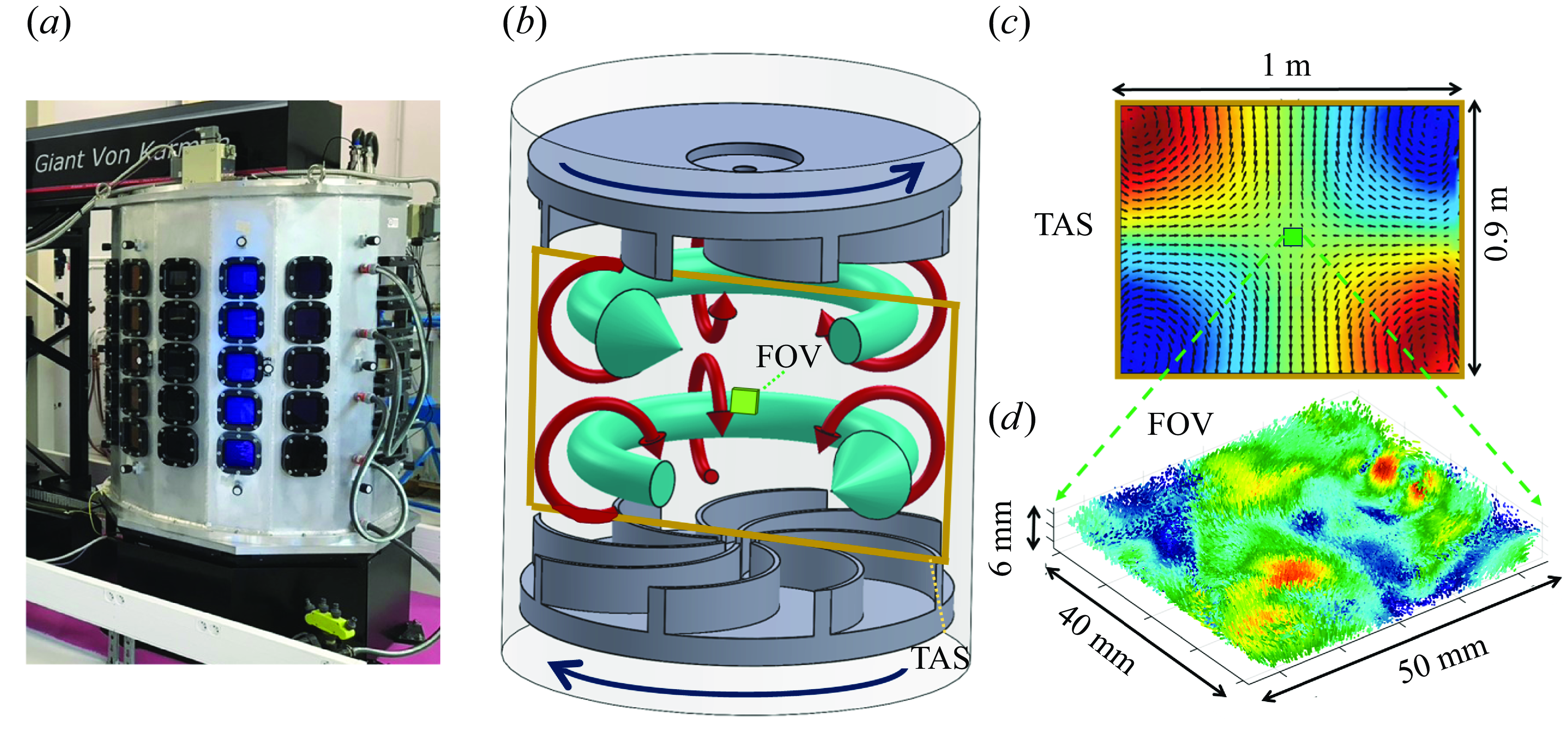
Figure 2. (a) Photo of the GvK experimental facility. (b) Schematic of the facility showing the direction of impeller rotation and time-averaged flow. Two tori revolve in the same direction as their nearest impeller, which induce counter-rotating vortices that create the turbulent shear layer where the field of view (FOV) is located. (c) Time-averaged slice (TAS) shows the steady-state velocity field in the meridional plane and the relative size and position of the FOV (Cortet et al. Reference Cortet, Chiffaudel, Daviaud and Dubrulle2010). The arrows show the velocity vectors in the axial–radial plane, while colour maps to the azimuthal velocity from negative (blue) to positive (red). (d) One instant of the 80 000 particle trajectories found in the FOV. Colour indicates velocity magnitude normalised by the impeller tip velocity (0 = blue, 1 = red).
Time-resolved 3-D velocity fields are obtained using 4-D particle tracking velocimetry, whereby a high-speed laser (
 $30$
mJ pulse Nd-YLG) illuminates a volume (
$30$
mJ pulse Nd-YLG) illuminates a volume (
 $V = 50 \times 40 \times 6\, \textrm{mm}^{3}$
) at the centred FOV, which is recorded using four cameras (Phantom Miro m340: 4.1 Megapixel CMOS sensors, with
$V = 50 \times 40 \times 6\, \textrm{mm}^{3}$
) at the centred FOV, which is recorded using four cameras (Phantom Miro m340: 4.1 Megapixel CMOS sensors, with
 $10\,\unicode{x03BC} m$
square pixels). The particles used are spherical polystyrene particles of 5
$10\,\unicode{x03BC} m$
square pixels). The particles used are spherical polystyrene particles of 5
 $\unicode{x03BC}$
m diameter (Stokes number of
$\unicode{x03BC}$
m diameter (Stokes number of
 $S_{t_{\tau _{\eta }}} \leqslant 8.1 \times 10^{-5}$
for all cases). Particle tracks are obtained using the Davis10 ‘shake-the-box’ algorithm (Schanz, Gesemann & Schröder Reference Schanz, Gesemann and Schröder2016). In house codes are then used to go from Lagrangian particle trajectories to Eulerian velocity fields. This process has been validated and described previously by Cheminet et al. (Reference Cheminet, Ostovan, Valori, Cuvier, Daviaud, Debue, Dubrulle, Foucaut and Laval2021). In short, a regularised B-spline filter is first applied on the Lagrangian trajectories to smooth out temporal noise on the tracks. Then a second regularised B-spline interpolation scheme (Gesemann et al. Reference Gesemann, Huhn, Schanz and Schröder2016) is used to project the velocity field onto a regular Eulerian grid.
$S_{t_{\tau _{\eta }}} \leqslant 8.1 \times 10^{-5}$
for all cases). Particle tracks are obtained using the Davis10 ‘shake-the-box’ algorithm (Schanz, Gesemann & Schröder Reference Schanz, Gesemann and Schröder2016). In house codes are then used to go from Lagrangian particle trajectories to Eulerian velocity fields. This process has been validated and described previously by Cheminet et al. (Reference Cheminet, Ostovan, Valori, Cuvier, Daviaud, Debue, Dubrulle, Foucaut and Laval2021). In short, a regularised B-spline filter is first applied on the Lagrangian trajectories to smooth out temporal noise on the tracks. Then a second regularised B-spline interpolation scheme (Gesemann et al. Reference Gesemann, Huhn, Schanz and Schröder2016) is used to project the velocity field onto a regular Eulerian grid.
The spatial resolution of our data is in turn determined by the number of particles in the FOV (
 $N_p \approx$
80 000 on average) where the mean inter-particle distance is:
$N_p \approx$
80 000 on average) where the mean inter-particle distance is:
 $\Delta x_p = (V / N_p)^{1/3}$
. When keeping constant flow and diagnostic parameters, increasing/decreasing the rotation frequency has the effect of physically decreasing/increasing the Kolmogorov length (
$\Delta x_p = (V / N_p)^{1/3}$
. When keeping constant flow and diagnostic parameters, increasing/decreasing the rotation frequency has the effect of physically decreasing/increasing the Kolmogorov length (
 $\eta$
) and time (
$\eta$
) and time (
 $\tau _\eta$
) scales, and thus the effective resolution:
$\tau _\eta$
) scales, and thus the effective resolution:
 $\Delta x_p / \eta$
. The simultaneous high
$\Delta x_p / \eta$
. The simultaneous high
 $Re$
, high resolution nature of these data can be seen in table 1, made notable by the fact that previous works on the morphology of 3D HIT turbulent data have typically been numerical (Buaria & Pumir Reference Buaria and Pumir2022). Other relevant experimental parameters displayed in table 1 are defined below. Here,
$Re$
, high resolution nature of these data can be seen in table 1, made notable by the fact that previous works on the morphology of 3D HIT turbulent data have typically been numerical (Buaria & Pumir Reference Buaria and Pumir2022). Other relevant experimental parameters displayed in table 1 are defined below. Here,
 $\langle \epsilon \rangle$
is an estimate for the average dissipation rate, found using torque meters located on the impeller shafts (Kuzzay, Faranda & Dubrulle Reference Kuzzay, Faranda and Dubrulle2015). The integral time scale is
$\langle \epsilon \rangle$
is an estimate for the average dissipation rate, found using torque meters located on the impeller shafts (Kuzzay, Faranda & Dubrulle Reference Kuzzay, Faranda and Dubrulle2015). The integral time scale is
 $T_i$
, while the Taylor Reynolds number (
$T_i$
, while the Taylor Reynolds number (
 $Re_{\lambda }$
) was computed from the measured root-mean-square (r.m.s.) velocity, assuming homogeneity. The relevant frequencies shown are the data acquisition frequency and impeller rotation frequency,
$Re_{\lambda }$
) was computed from the measured root-mean-square (r.m.s.) velocity, assuming homogeneity. The relevant frequencies shown are the data acquisition frequency and impeller rotation frequency,
 $F_a$
and
$F_a$
and
 $F$
, respectively.
$F$
, respectively.
Table 1. Table of experimental parameters for the three GvK data sets. The colours indicate the datasets used later in the conditioning analysis. When compared against each other, the two datasets will be differentiated by bounding boxes of their corresponding colour.

The ratio of
 $\tau _{d} / \tau _{\eta }$
is the mean de-correlation time of the time-resolved velocity fields relative to the Kolmogorov time scale. As this work is statistical and the data acquisition is time resolved, we sample our velocity fields to produce snapshots that are statistically independent temporally. The time step between independent snapshots is determined by
$\tau _{d} / \tau _{\eta }$
is the mean de-correlation time of the time-resolved velocity fields relative to the Kolmogorov time scale. As this work is statistical and the data acquisition is time resolved, we sample our velocity fields to produce snapshots that are statistically independent temporally. The time step between independent snapshots is determined by
 $\tau _{d}$
, and the resulting number of statistically independent flow fields for each case is
$\tau _{d}$
, and the resulting number of statistically independent flow fields for each case is
 $N$
. To find
$N$
. To find
 $N$
, the autocorrelation function (
$N$
, the autocorrelation function (
 $ACF_{ii}(\tau ) = \langle v_i(t) v_i(t+\tau ) \rangle / \langle v_i^2(t) \rangle$
) is first computed at an array of points in the measurement volume for each, mean subtracted, Eulerian velocity component,
$ACF_{ii}(\tau ) = \langle v_i(t) v_i(t+\tau ) \rangle / \langle v_i^2(t) \rangle$
) is first computed at an array of points in the measurement volume for each, mean subtracted, Eulerian velocity component,
 $v_i$
. The de-correlation time
$v_i$
. The de-correlation time
 $\tau _{d}$
is then found via
$\tau _{d}$
is then found via
 $\tau _{d} = \langle ACF(\tau ) = 0.025 \rangle$
, or in other words the average de-correlation time of the velocity
$\tau _{d} = \langle ACF(\tau ) = 0.025 \rangle$
, or in other words the average de-correlation time of the velocity
 $ACF$
. Then,
$ACF$
. Then,
 $N$
is set using the necessary spacing provided by
$N$
is set using the necessary spacing provided by
 $\tau _d$
. As this parameter controls the sampling of the experimental results, we have tested the sensitivity to this parameter. We have increased
$\tau _d$
. As this parameter controls the sampling of the experimental results, we have tested the sensitivity to this parameter. We have increased
 $\tau _d$
up to a factor of five (thereby decreasing the number of statistical snapshots), and have observed that the trends and results presented below do not show any notable change.
$\tau _d$
up to a factor of five (thereby decreasing the number of statistical snapshots), and have observed that the trends and results presented below do not show any notable change.
Finally, we note that, in order to present results which are statistically converged, this work focuses on results only from the two highest
 $Re$
cases of table 1, with a particular focus on the highest
$Re$
cases of table 1, with a particular focus on the highest
 $Re$
case. This is done to take advantage of the large
$Re$
case. This is done to take advantage of the large
 $N$
for this case, as noted in table 1. However, this raises the question as to whether the most extreme velocity gradients are properly resolved, since this case is also the one with the poorest resolution. In order to evaluate whether the gradients are properly resolved the authors have run the same analysis for all
$N$
for this case, as noted in table 1. However, this raises the question as to whether the most extreme velocity gradients are properly resolved, since this case is also the one with the poorest resolution. In order to evaluate whether the gradients are properly resolved the authors have run the same analysis for all
 $Re$
cases. Aside from obvious convergence issues at the lowest
$Re$
cases. Aside from obvious convergence issues at the lowest
 $Re$
, we have confirmed that the trends and results discussed in § 4 are very similar for the highest and middle
$Re$
, we have confirmed that the trends and results discussed in § 4 are very similar for the highest and middle
 $Re$
cases. In fact, we will only present results from the middle
$Re$
cases. In fact, we will only present results from the middle
 $Re$
case when there is a notable difference in results as compared with the highest
$Re$
case when there is a notable difference in results as compared with the highest
 $Re$
case. When this is done, the results will be respectively bounded in a blue box and orange box for the middle and largest
$Re$
case. When this is done, the results will be respectively bounded in a blue box and orange box for the middle and largest
 $Re$
case, as indicated in table 1. Thus, if not explicitly shown, one should assume that results for the largest case (
$Re$
case, as indicated in table 1. Thus, if not explicitly shown, one should assume that results for the largest case (
 $Re$
= 1 56 719) are the same as those for the middle case (
$Re$
= 1 56 719) are the same as those for the middle case (
 $Re$
= 39 180). Unfortunately, the conditioned results from the lowest
$Re$
= 39 180). Unfortunately, the conditioned results from the lowest
 $Re$
case suffer greatly from a lack of statistical convergence and they are largely not included in this work. In addition to issues of convergence, there also exists error arising from the diagnostics and algorithms used to convert 2-D particle images to a Eulerian velocity field. Unfortunately, explicitly quantifying this error is challenging and would likely require DNS. In light of this, we reference the directly relevant work of Sciacchitano, Leclaire & Schröder (Reference Sciacchitano, Leclaire and Schröder2025) to estimate the measurement errors associated with this work. This work studied the effect of the algorithms and diagnostic set-up used in the present paper using relevant synthetic data. Their results show that one should expect velocity and velocity-gradient errors of the order of 3 %–10
$Re$
case suffer greatly from a lack of statistical convergence and they are largely not included in this work. In addition to issues of convergence, there also exists error arising from the diagnostics and algorithms used to convert 2-D particle images to a Eulerian velocity field. Unfortunately, explicitly quantifying this error is challenging and would likely require DNS. In light of this, we reference the directly relevant work of Sciacchitano, Leclaire & Schröder (Reference Sciacchitano, Leclaire and Schröder2025) to estimate the measurement errors associated with this work. This work studied the effect of the algorithms and diagnostic set-up used in the present paper using relevant synthetic data. Their results show that one should expect velocity and velocity-gradient errors of the order of 3 %–10
 $\, \%$
and 10 %–15
$\, \%$
and 10 %–15
 $\, \%$
, respectively. Due to the specific algorithm and the high seeding density (
$\, \%$
, respectively. Due to the specific algorithm and the high seeding density (
 $\approx$
0.1 particle per pixel) used here, one expects the error in this work to be on the lower end of these ranges.
$\approx$
0.1 particle per pixel) used here, one expects the error in this work to be on the lower end of these ranges.
3. Quantities of interest
The analysis of the experimental data revolves primarily around three quantities and their products. These are the strain-rate tensor
 $\unicode{x1D64E}$
, the vorticity vector
$\unicode{x1D64E}$
, the vorticity vector
 $\boldsymbol{\omega }$
and the scalar parameter ‘
$\boldsymbol{\omega }$
and the scalar parameter ‘
 $\mathcal{D}_\ell$
’ (defined below in (3.3)). Again, note that we have sampled the time-resolved data to obtain statistically independent data.
$\mathcal{D}_\ell$
’ (defined below in (3.3)). Again, note that we have sampled the time-resolved data to obtain statistically independent data.
Due to their importance in the production of vortex stretching and dissipation, the alignment of
 $\boldsymbol{\omega }$
and the principal axes of
$\boldsymbol{\omega }$
and the principal axes of
 $\unicode{x1D64E}$
are of interest. The eigenvectors of
$\unicode{x1D64E}$
are of interest. The eigenvectors of
 $\unicode{x1D64E}$
(
$\unicode{x1D64E}$
(
 $\boldsymbol{e}_1 \,$
,
$\boldsymbol{e}_1 \,$
,
 $\boldsymbol{e}_2 \,$
,
$\boldsymbol{e}_2 \,$
,
 $\boldsymbol{e}_3 \,$
) have three corresponding eigenvalues which are defined such that
$\boldsymbol{e}_3 \,$
) have three corresponding eigenvalues which are defined such that
 $\lambda _1 \,$
 $\, \geqslant$
 $\lambda _2 \,$
 $\, \geqslant$
 $\lambda _3 \,$
. To find the degree of
$\lambda _3 \,$
. To find the degree of
 $\boldsymbol{\omega }$
 $\unicode{x1D64E}$
alignment, we consider the alignment cosine,
$\unicode{x1D64E}$
alignment, we consider the alignment cosine,
 $C_i$
, between the vorticity unit vector,
$C_i$
, between the vorticity unit vector,
 $\hat {\boldsymbol{\omega }}$
, and the three principal axes of
$\hat {\boldsymbol{\omega }}$
, and the three principal axes of
 $\unicode{x1D64E}$
such that
$\unicode{x1D64E}$
such that
 \begin{equation} C_i = |\! \cos ( \boldsymbol{e_i \cdot \hat {\omega }} ) | . \end{equation}
Then,
 $C_i$
is bounded between 0 and 1 for each principal direction, with
$C_i$
is bounded between 0 and 1 for each principal direction, with
 $\boldsymbol{\omega }$
being perpendicular or parallel to
$\boldsymbol{\omega }$
being perpendicular or parallel to
 $\boldsymbol{e_i}$
for values of 0 and 1, respectively.
$\boldsymbol{e_i}$
for values of 0 and 1, respectively.
Incompressible continuity (
 $\boldsymbol{\nabla \cdot u}$
= 0) imposes an additional constraint on the eigenvalues of
$\boldsymbol{\nabla \cdot u}$
= 0) imposes an additional constraint on the eigenvalues of
 $\unicode{x1D64E}$
such that
$\unicode{x1D64E}$
such that
 $\lambda _1 \,$
+
$\lambda _1 \,$
+
 $\lambda _2 \,$
+
$\lambda _2 \,$
+
 $\lambda _3 \,$
= 0. Thus, as the most extensive strain eigenvector
$\lambda _3 \,$
= 0. Thus, as the most extensive strain eigenvector
 $\boldsymbol{e}_1 \,$
is always positive (
$\boldsymbol{e}_1 \,$
is always positive (
 $\lambda _1 \;\gt\; 0$
) and the most compressive strain eigenvector
$\lambda _1 \;\gt\; 0$
) and the most compressive strain eigenvector
 $\boldsymbol{e}_3 \,$
is always negative (
$\boldsymbol{e}_3 \,$
is always negative (
 $\lambda _3 \;\lt\; 0$
), the value of
$\lambda _3 \;\lt\; 0$
), the value of
 $\lambda _2 \,$
will change sign depending on the local flow behaviour. We quantify the sign and relative amplitude of
$\lambda _2 \,$
will change sign depending on the local flow behaviour. We quantify the sign and relative amplitude of
 $\lambda _2 \,$
using
$\lambda _2 \,$
using
 \begin{equation} \beta = \sqrt {6}\lambda _2 \, / \sqrt {\lambda _1^2 + \lambda _2^2 + \lambda _3^2} . \end{equation}
We will also report statistics on the second and third invariants of the velocity-gradient tensor,
 $Q$
and
$Q$
and
 $R$
, respectively. Here,
$R$
, respectively. Here,
 $Q= ({1}/{4}) \omega _i \omega _i - ({1}/{2}) S_{ij}S_{ij}$
and
$Q= ({1}/{4}) \omega _i \omega _i - ({1}/{2}) S_{ij}S_{ij}$
and
 $R= -({1}/{3}) S_{ij}S_{jk}S_{ki} - ({1}/{4}) \omega _i S_{ij} \omega _j$
– the quantities whose joint distributions make up the aforementioned QR plot. Note that velocity derivatives are computed from the Eulerian field using a second-order central-differencing scheme.
$R= -({1}/{3}) S_{ij}S_{jk}S_{ki} - ({1}/{4}) \omega _i S_{ij} \omega _j$
– the quantities whose joint distributions make up the aforementioned QR plot. Note that velocity derivatives are computed from the Eulerian field using a second-order central-differencing scheme.
Finally, as we are interested in determining the morphology of the flow field around events which transfer large amounts of energy, we measure this energy transfer using the
 $\mathcal{D}_\ell$
parameter, a term generated in the ‘weak Kármán–Howarth–Monin equation’ (Dubrulle Reference Dubrulle2019). This is a scale- and space-dependent energy balance for the point-split kinetic energy,
$\mathcal{D}_\ell$
parameter, a term generated in the ‘weak Kármán–Howarth–Monin equation’ (Dubrulle Reference Dubrulle2019). This is a scale- and space-dependent energy balance for the point-split kinetic energy,
 $E^{\mathrm{\ell }}(\boldsymbol{x}) \equiv u_i u_i^\ell /2$
, developed in previous works by Onsager (Reference Onsager1949), Duchon & Robert (Reference Duchon and Robert2000), Dubrulle (Reference Dubrulle2019). The value of
$E^{\mathrm{\ell }}(\boldsymbol{x}) \equiv u_i u_i^\ell /2$
, developed in previous works by Onsager (Reference Onsager1949), Duchon & Robert (Reference Duchon and Robert2000), Dubrulle (Reference Dubrulle2019). The value of
 $E^\ell (x)$
changes across time, space and scale (
$E^\ell (x)$
changes across time, space and scale (
 $\ell$
) due to the transport of energy within the flow. In this work we are only interested in one term from the evolution equation of
$\ell$
) due to the transport of energy within the flow. In this work we are only interested in one term from the evolution equation of
 $E^\ell (x)$
, the inter-scale energy flux
$E^\ell (x)$
, the inter-scale energy flux
 \begin{equation} \mathcal{D}_\ell = \tfrac {1}{4}\int \nabla \phi ^\ell (\xi )\cdot \delta \boldsymbol{u} (\delta \boldsymbol{u})^2 \; d^3\boldsymbol{\xi }\, . \end{equation}
Here, the velocity increment, dependent on space (
 $\boldsymbol{x}$
) and increment distance (
$\boldsymbol{x}$
) and increment distance (
 $\boldsymbol{\xi }$
), is
$\boldsymbol{\xi }$
), is
 $\delta \boldsymbol{u} = \boldsymbol{u}(\boldsymbol{x}+\boldsymbol{\xi }) - \boldsymbol{u}(\boldsymbol{x})$
and
$\delta \boldsymbol{u} = \boldsymbol{u}(\boldsymbol{x}+\boldsymbol{\xi }) - \boldsymbol{u}(\boldsymbol{x})$
and
 $\phi ^\ell$
is a smooth, even, non-negative and spatially localised smoothing operator which effectively removes fluctuations on scales smaller than
$\phi ^\ell$
is a smooth, even, non-negative and spatially localised smoothing operator which effectively removes fluctuations on scales smaller than
 $\ell$
, meaning smaller
$\ell$
, meaning smaller
 $\ell$
results in less smoothing. In our case it is the following Gaussian function:
$\ell$
results in less smoothing. In our case it is the following Gaussian function:
 $\phi ^\ell (x) = \exp ( - {30x^2}/{2\ell ^2} ) / ( {2\pi \ell ^2}/{30} )^{1.5}.$
The scalar
$\phi ^\ell (x) = \exp ( - {30x^2}/{2\ell ^2} ) / ( {2\pi \ell ^2}/{30} )^{1.5}.$
The scalar
 $\mathcal{D}_\ell$
is the non-viscous inter-scale transfer term, i.e. the local (in space and time) rate of energy transfer from scales larger than
$\mathcal{D}_\ell$
is the non-viscous inter-scale transfer term, i.e. the local (in space and time) rate of energy transfer from scales larger than
 $\ell$
to scales smaller than
$\ell$
to scales smaller than
 $\ell$
. It adopts the convection that positive
$\ell$
. It adopts the convection that positive
 $\mathcal{D}_\ell$
values indicate energy transfer to scales below
$\mathcal{D}_\ell$
values indicate energy transfer to scales below
 $\ell$
and vice versa (Dubrulle Reference Dubrulle2019; Debue et al. Reference Debue, Valori, Cuvier, Daviaud, Foucaut, Laval, Wiertel, Padilla and Dubrulle2021). In the limit of
$\ell$
and vice versa (Dubrulle Reference Dubrulle2019; Debue et al. Reference Debue, Valori, Cuvier, Daviaud, Foucaut, Laval, Wiertel, Padilla and Dubrulle2021). In the limit of
 $\ell \to 0$
,
$\ell \to 0$
,
 $\mathcal{D}_\ell$
can also be thought of as an inertial dissipation arising from the irregularity of the velocity field, or in other words, the non-viscous contribution to dissipation due to velocity roughness (Duchon & Robert Reference Duchon and Robert2000).
$\mathcal{D}_\ell$
can also be thought of as an inertial dissipation arising from the irregularity of the velocity field, or in other words, the non-viscous contribution to dissipation due to velocity roughness (Duchon & Robert Reference Duchon and Robert2000).
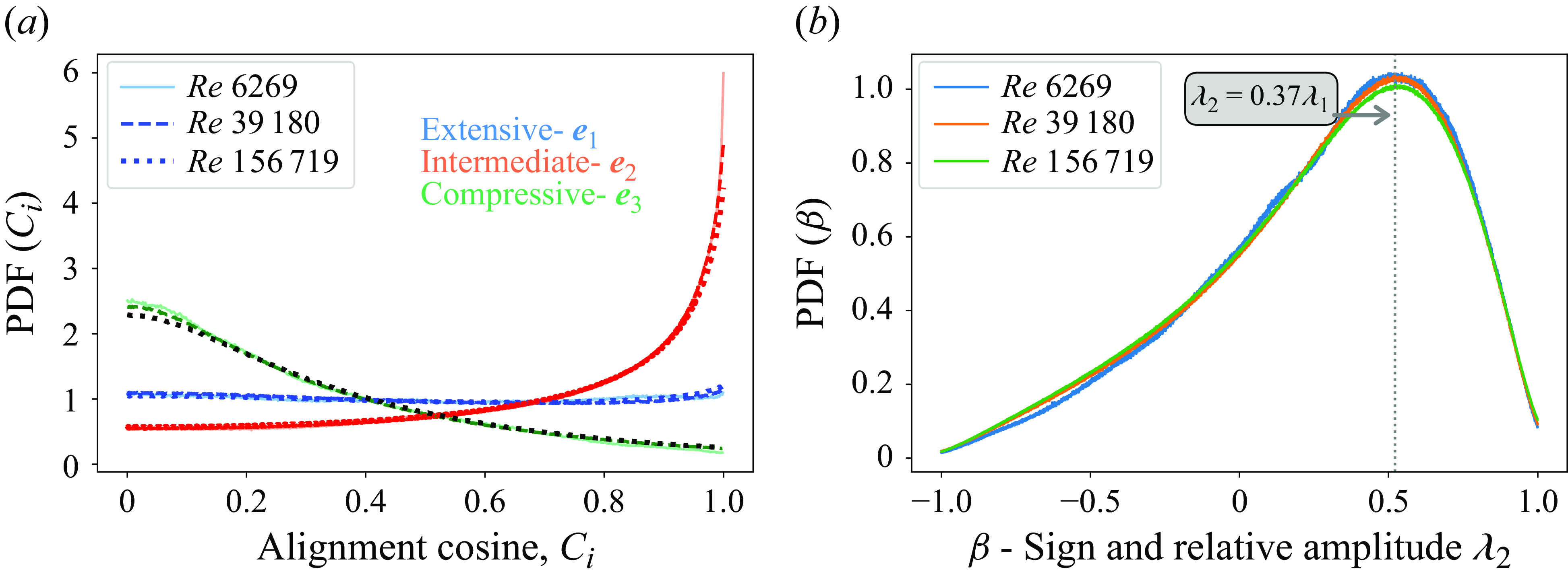
Figure 3. Distributions of
 $C_i$
and
$C_i$
and
 $\beta$
for a range of
$\beta$
for a range of
 $Re$
. (a) Alignment cosine (
$Re$
. (a) Alignment cosine (
 $C_i$
) distributions of the strain-rate tensor eigenvectors and the vorticity vector. For each eigenvector, different
$C_i$
) distributions of the strain-rate tensor eigenvectors and the vorticity vector. For each eigenvector, different
 $Re$
are indicated by shades of the same colour. (b) Distributions of the relative amplitude of the intermediate
$Re$
are indicated by shades of the same colour. (b) Distributions of the relative amplitude of the intermediate
 $\unicode{x1D64E}$
eigenvector (
$\unicode{x1D64E}$
eigenvector (
 $\beta$
) for different
$\beta$
) for different
 $Re$
. The value of
$Re$
. The value of
 $\lambda _2 \,$
(relative to
$\lambda _2 \,$
(relative to
 $\lambda _1 \,$
) corresponding to the most probable
$\lambda _1 \,$
) corresponding to the most probable
 $\beta$
value is shown in the grey box.
$\beta$
value is shown in the grey box.
4. Results
4.1. Unconditioned statistics
Figure 3 shows the unconditioned probability density functions (PDFs) of the alignment cosine (
 $C_i$
-(3.1)) and the intermediate eigenvector sign and amplitude (
$C_i$
-(3.1)) and the intermediate eigenvector sign and amplitude (
 $\beta$
-(3.2)) for a range of
$\beta$
-(3.2)) for a range of
 $Re$
. The results agree well with the vast amount of previous work, the majority of which was done using DNS on HIT flows. We observe the common trend of
$Re$
. The results agree well with the vast amount of previous work, the majority of which was done using DNS on HIT flows. We observe the common trend of
 $\boldsymbol{\omega }$
alignment with the intermediate
$\boldsymbol{\omega }$
alignment with the intermediate
 $\unicode{x1D64E}$
eigenvector, which is generally positive (extensive). We also observe the lack of any preferential alignment with the extensive eigenvector (
$\unicode{x1D64E}$
eigenvector, which is generally positive (extensive). We also observe the lack of any preferential alignment with the extensive eigenvector (
 $\boldsymbol{e}_1 \,$
) and a preference for perpendicularity between
$\boldsymbol{e}_1 \,$
) and a preference for perpendicularity between
 $\boldsymbol{\omega }$
and
$\boldsymbol{\omega }$
and
 $\boldsymbol{e}_3 \,$
, the principal compressive axis of
$\boldsymbol{e}_3 \,$
, the principal compressive axis of
 $\unicode{x1D64E}$
. See figure 1(a) for a schematic showing this preferred nominal alignment of an idealised vortex in a strain field. While the preference for
$\unicode{x1D64E}$
. See figure 1(a) for a schematic showing this preferred nominal alignment of an idealised vortex in a strain field. While the preference for
 $\lambda _2\;\gt\; 0$
was shown by Betchov (Reference Betchov1956) to be necessary for net enstrophy production in a turbulent flow, the predominant
$\lambda _2\;\gt\; 0$
was shown by Betchov (Reference Betchov1956) to be necessary for net enstrophy production in a turbulent flow, the predominant
 $\boldsymbol{\omega }$
–
$\boldsymbol{\omega }$
–
 $\boldsymbol{e}_2 \,$
alignment has been used to explain the limited vorticity growth rates, as compared with those of passive scalars, observed in turbulence (Elsinga & Marusic Reference Elsinga and Marusic2010).
$\boldsymbol{e}_2 \,$
alignment has been used to explain the limited vorticity growth rates, as compared with those of passive scalars, observed in turbulence (Elsinga & Marusic Reference Elsinga and Marusic2010).
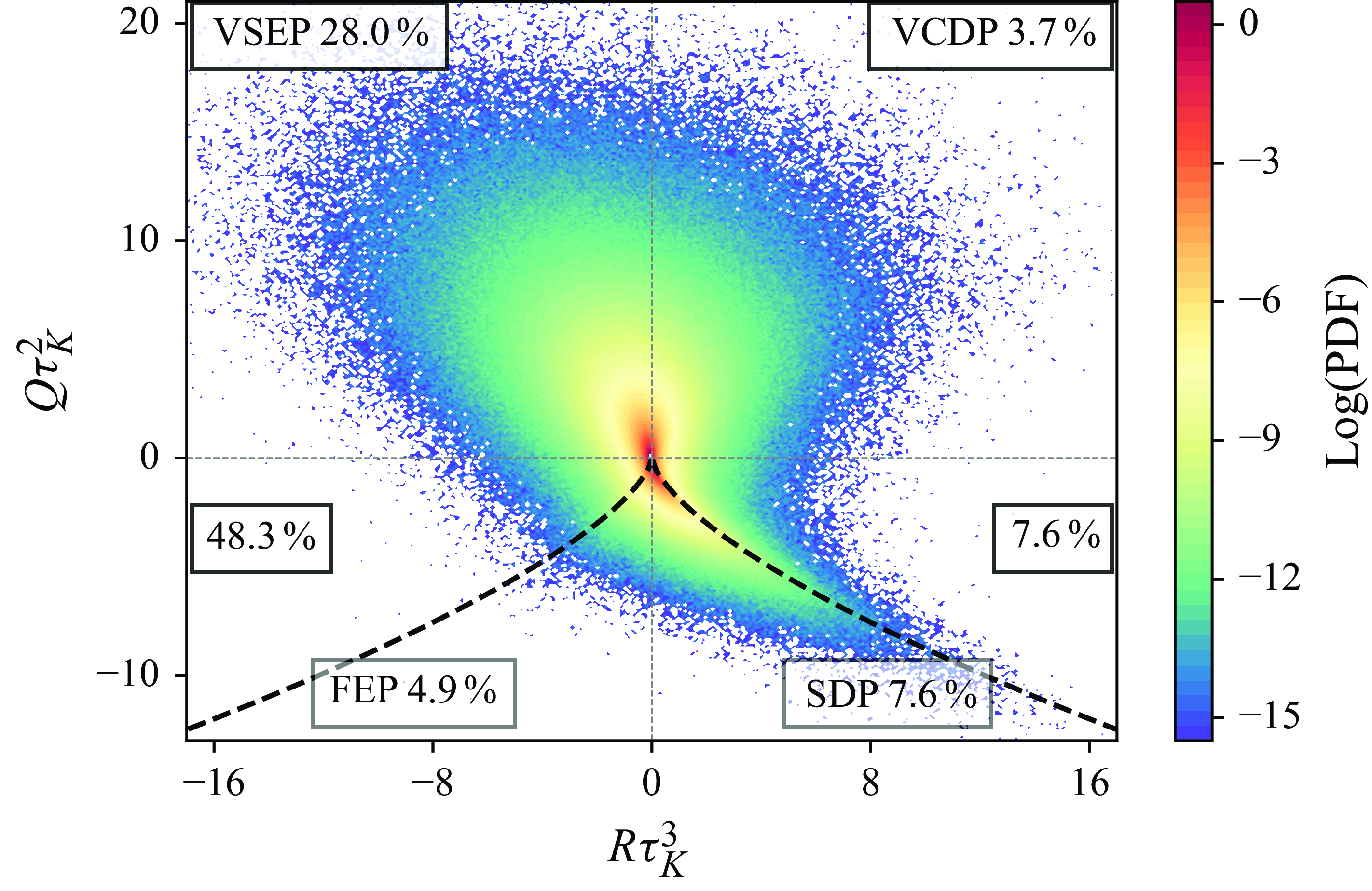
Figure 4. A QR plot of the non-conditioned turbulent flow at
 $Re$
= 156 719. The dashed line is the Vieillefosse line: VSEP (vortex-stretching enstrophy production), VCDP (vortex-compressing dissipation production), SDP (sheet dissipation production) and FDP (filament enstrophy production) indicate different topological regions of QR space. The percentage of total events in each region is also indicated by the text boxes. The plot is non-dimensionalised by the appropriate powers of
$Re$
= 156 719. The dashed line is the Vieillefosse line: VSEP (vortex-stretching enstrophy production), VCDP (vortex-compressing dissipation production), SDP (sheet dissipation production) and FDP (filament enstrophy production) indicate different topological regions of QR space. The percentage of total events in each region is also indicated by the text boxes. The plot is non-dimensionalised by the appropriate powers of
 $\tau _K$
, the Kolmogorov time scale.
$\tau _K$
, the Kolmogorov time scale.
The unconditioned joint PDF of the velocity-gradient invariants
 $Q$
and
$Q$
and
 $R$
for the case of
$R$
for the case of
 $Re = 156\ 719$
is shown in the QR plot of figure 4. The other two
$Re = 156\ 719$
is shown in the QR plot of figure 4. The other two
 $Re$
cases exhibit unconditioned QR plots of very similar shape, and are thus not shown. Again due to incompressibility, the first invariant,
$Re$
cases exhibit unconditioned QR plots of very similar shape, and are thus not shown. Again due to incompressibility, the first invariant,
 $P$
, of the velocity gradient is zero. As such, one can define a line (
$P$
, of the velocity gradient is zero. As such, one can define a line (
 $D$
) which separates the real and complex roots of the velocity-gradient tensor as:
$D$
) which separates the real and complex roots of the velocity-gradient tensor as:
 $D = Q^3 +(27/4)R^2$
. Meaning that
$D = Q^3 +(27/4)R^2$
. Meaning that
 $D\gt 0$
represents swirling flow topology, while regions with
$D\gt 0$
represents swirling flow topology, while regions with
 $D\lt 0$
are strain dominated. This is shown as the dashed line in figure 4 and is better known as the ‘Vieillefosse line/tail’ (Vieillefosse Reference Vieillefosse1984). The QR plot can be further partitioned based on the sign of
$D\lt 0$
are strain dominated. This is shown as the dashed line in figure 4 and is better known as the ‘Vieillefosse line/tail’ (Vieillefosse Reference Vieillefosse1984). The QR plot can be further partitioned based on the sign of
 $R$
and
$R$
and
 $Q$
, where positive and negative
$Q$
, where positive and negative
 $R$
indicate unstable and stable solutions, respectively, while positive and negative
$R$
indicate unstable and stable solutions, respectively, while positive and negative
 $Q$
indicate enstrophy-dominated and strain-dominated regions, respectively (Chevillard & Meneveau Reference Chevillard and Meneveau2006; Chevillard et al. Reference Chevillard, Meneveau, Biferale and Toschi2008; Elsinga & Marusic Reference Elsinga and Marusic2010). One can also interpret the sign of
$Q$
indicate enstrophy-dominated and strain-dominated regions, respectively (Chevillard & Meneveau Reference Chevillard and Meneveau2006; Chevillard et al. Reference Chevillard, Meneveau, Biferale and Toschi2008; Elsinga & Marusic Reference Elsinga and Marusic2010). One can also interpret the sign of
 $R$
morphologically, where
$R$
morphologically, where
 $R \lt 0$
indicates a stretching principal direction (i.e. vortex stretching) and
$R \lt 0$
indicates a stretching principal direction (i.e. vortex stretching) and
 $R \gt 0$
indicates a compressive principal direction (strain self-amplification or vortex compression).
$R \gt 0$
indicates a compressive principal direction (strain self-amplification or vortex compression).
The QR plot can therefore be divided into four (or six) regions, each corresponding to a solution type of the characteristic equation of the velocity-gradient tensor’s eigenvalues, which correspond to different flow topologies. The top left region of the QR plot in figure 4 labelled VSEP (V
 $R \lt 0,\; Q \gt D$
) is characterised by enstrophy-producing regions of the flow driven by stable vortex-stretching topologies. The top right region labelled VCDP (
$R \lt 0,\; Q \gt D$
) is characterised by enstrophy-producing regions of the flow driven by stable vortex-stretching topologies. The top right region labelled VCDP (
 $R \gt 0,\; Q \gt D$
) contains regions of the flow that produce dissipation via unstable vortex-compression topologies. Correspondingly, the bottom right region labelled SDP (
$R \gt 0,\; Q \gt D$
) contains regions of the flow that produce dissipation via unstable vortex-compression topologies. Correspondingly, the bottom right region labelled SDP (
 $R \gt 0,\; Q \lt D$
) pertains to unstable saddle-node, or sheet, topologies which tend to produce dissipation. Finally, the bottom left region labelled FEP (
$R \gt 0,\; Q \lt D$
) pertains to unstable saddle-node, or sheet, topologies which tend to produce dissipation. Finally, the bottom left region labelled FEP (
 $R \lt 0,\; Q \lt D$
) produces enstrophy via stable node, or filament topologies (Chong, Perry & Cantwell Reference Chong, Perry and Cantwell1990; Chevillard & Meneveau Reference Chevillard and Meneveau2006; Chevillard et al. Reference Chevillard, Meneveau, Biferale and Toschi2008; Elsinga & Marusic Reference Elsinga and Marusic2010; Danish & Meneveau Reference Danish and Meneveau2018; Debue et al. Reference Debue, Valori, Cuvier, Daviaud, Foucaut, Laval, Wiertel, Padilla and Dubrulle2021). We direct the reader to the work of Suman & Girimaji (Reference Suman and Girimaji2010) for a more nuanced explanation of stability/instability in the QR plot. One can additionally split the VSEP and VCDP regions into
$R \lt 0,\; Q \lt D$
) produces enstrophy via stable node, or filament topologies (Chong, Perry & Cantwell Reference Chong, Perry and Cantwell1990; Chevillard & Meneveau Reference Chevillard and Meneveau2006; Chevillard et al. Reference Chevillard, Meneveau, Biferale and Toschi2008; Elsinga & Marusic Reference Elsinga and Marusic2010; Danish & Meneveau Reference Danish and Meneveau2018; Debue et al. Reference Debue, Valori, Cuvier, Daviaud, Foucaut, Laval, Wiertel, Padilla and Dubrulle2021). We direct the reader to the work of Suman & Girimaji (Reference Suman and Girimaji2010) for a more nuanced explanation of stability/instability in the QR plot. One can additionally split the VSEP and VCDP regions into
 $Q \gt 0$
and
$Q \gt 0$
and
 $0 \gt Q \gt D$
where the former contains swirling topologies in regions dominated by enstrophy, and the latter, while still containing swirling topologies, are regions where strain is more prevalent (Danish & Meneveau Reference Danish and Meneveau2018).
$0 \gt Q \gt D$
where the former contains swirling topologies in regions dominated by enstrophy, and the latter, while still containing swirling topologies, are regions where strain is more prevalent (Danish & Meneveau Reference Danish and Meneveau2018).

Figure 5. The PDFs of mean-normalised energy transfer (
 $\mathcal{D}_\ell$
) to and from scale
$\mathcal{D}_\ell$
) to and from scale
 $\ell$
for a range of scales at (a)
$\ell$
for a range of scales at (a)
 $Re$
= 156 719 and (b)
$Re$
= 156 719 and (b)
 $Re$
= 39 180. The insets are a zoom of the distributions near the peak, showing the collapse of the distributions and the positive skewness.
$Re$
= 39 180. The insets are a zoom of the distributions near the peak, showing the collapse of the distributions and the positive skewness.
The resulting tear-drop shape of the QR plot (with the pointed portion along the positive/right Vieillefosse tail) in figure 4 is now one of the most notable features in a turbulent flow (Elsinga & Marusic Reference Elsinga and Marusic2010). This familiar shape indicates that, on average, turbulent flows generate enstrophy via vortex stretching and produce dissipation via sheets and compressive vortices in strain-dominated regions. The ubiquity of the results shown in figures 3 and 4 may be interpreted as universal statistical manifestations of the structure of turbulent flows (Tsinober Reference Tsinober2009). Additionally, one should note that a random, divergence-free flow field would result in a shape symmetric about the R axis (Elsinga & Marusic Reference Elsinga and Marusic2010), which is of course not the case here, highlighting the very non-Gaussian nature of turbulence. One should note that, for the quantities shown in figures 3 and 4, and all subsequent velocity-gradient data, we estimate an error of
 $\approx\! 10\, \%$
as discussed in § 2 (Sciacchitano et al. Reference Sciacchitano, Leclaire and Schröder2025).
$\approx\! 10\, \%$
as discussed in § 2 (Sciacchitano et al. Reference Sciacchitano, Leclaire and Schröder2025).
Finally, we quantify the scale-to-scale energy transfer in our flow using
 $\mathcal{D}_\ell$
, previously defined in (3.3). Again referencing the work of Sciacchitano et al. (Reference Sciacchitano, Leclaire and Schröder2025), we estimate the error on
$\mathcal{D}_\ell$
, previously defined in (3.3). Again referencing the work of Sciacchitano et al. (Reference Sciacchitano, Leclaire and Schröder2025), we estimate the error on
 $\mathcal{D}_\ell$
data to be
$\mathcal{D}_\ell$
data to be
 $\approx\! 5\, \%$
as it is derived directly from the velocity increments. The distribution of
$\approx\! 5\, \%$
as it is derived directly from the velocity increments. The distribution of
 $\mathcal{D}_\ell$
is shown in figure 5
a for a range of scales at the highest
$\mathcal{D}_\ell$
is shown in figure 5
a for a range of scales at the highest
 $Re$
(1 56 719), and likewise for the lower
$Re$
(1 56 719), and likewise for the lower
 $Re$
case in figure 5(b). The insets in figure 5 show zooms of the distributions near the peak and display more clearly the asymmetry toward positive values and the collapse across scales for the most probable events. One can see the highly non-Gaussian nature of the distribution, as the long tails indicate energy transfer events up to three orders of magnitude higher than the mean. These wide tails are known to be quite characteristic of
$Re$
case in figure 5(b). The insets in figure 5 show zooms of the distributions near the peak and display more clearly the asymmetry toward positive values and the collapse across scales for the most probable events. One can see the highly non-Gaussian nature of the distribution, as the long tails indicate energy transfer events up to three orders of magnitude higher than the mean. These wide tails are known to be quite characteristic of
 $\mathcal{D}_\ell$
distributions and have been found to be independent of the normalising factor (mean, standard deviation or global dissipation). Table 2 is also included to further characterise the distribution of
$\mathcal{D}_\ell$
distributions and have been found to be independent of the normalising factor (mean, standard deviation or global dissipation). Table 2 is also included to further characterise the distribution of
 $\mathcal{D}_\ell$
across scale. The ratio of r.m.s. value to the mean is shown, along with the skewness, S, and excess kurtosis, K. The table also displays the probability of the occurrence of events 10 or 100 times the mean, which were computed using the Cumulative Distribution Function of the distributions displayed in figure 5. Additionally, previous works such as Debue et al. (Reference Debue, Shukla, Kuzzay, Faranda, Saw, Daviaud and Dubrulle2018b
, Reference Debue, Valori, Cuvier, Daviaud, Foucaut, Laval, Wiertel, Padilla and Dubrulle2021) have shown that
$\mathcal{D}_\ell$
across scale. The ratio of r.m.s. value to the mean is shown, along with the skewness, S, and excess kurtosis, K. The table also displays the probability of the occurrence of events 10 or 100 times the mean, which were computed using the Cumulative Distribution Function of the distributions displayed in figure 5. Additionally, previous works such as Debue et al. (Reference Debue, Shukla, Kuzzay, Faranda, Saw, Daviaud and Dubrulle2018b
, Reference Debue, Valori, Cuvier, Daviaud, Foucaut, Laval, Wiertel, Padilla and Dubrulle2021) have shown that
 $\mathcal{D}_\ell$
is largest in regions of the flow which display the smallest amounts of dissipation, while also being closely correlated with the most intermittent patches in a turbulent field. Other findings from these works indicate that
$\mathcal{D}_\ell$
is largest in regions of the flow which display the smallest amounts of dissipation, while also being closely correlated with the most intermittent patches in a turbulent field. Other findings from these works indicate that
 $\mathcal{D}_\ell$
behaves as intermittently in the dissipation range as it does in the inertial range.
$\mathcal{D}_\ell$
behaves as intermittently in the dissipation range as it does in the inertial range.
Table 2. Table of parameters characterising the distributions of
 $\mathcal{D}_\ell$
shown in figure 5. The highlighted scales indicate those which are used in the conditioned statistics later on. Orange and blue indicate the scale analysed at
$\mathcal{D}_\ell$
shown in figure 5. The highlighted scales indicate those which are used in the conditioned statistics later on. Orange and blue indicate the scale analysed at
 $Re$
= 156 719 and
$Re$
= 156 719 and
 $Re$
= 39 180, respectively.
$Re$
= 39 180, respectively.
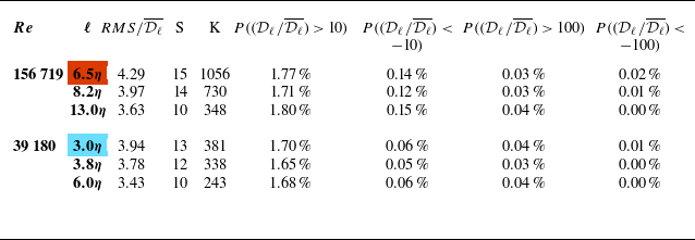
Three things should be noted regarding figure 5. The first is that the relative amplitudes of the largest events increase as the scale decreases. Second, positive values of
 $\mathcal{D}_\ell$
(which we will call
$\mathcal{D}_\ell$
(which we will call
 $\mathcal{D}_{\boldsymbol{\vee }}$
) indicate ‘direct’ cascade or downscale energy transfer events, while negative values (
$\mathcal{D}_{\boldsymbol{\vee }}$
) indicate ‘direct’ cascade or downscale energy transfer events, while negative values (
 $\mathcal{D}_{\boldsymbol{\wedge }}$
) indicate ‘inverse’ cascade or upscale energy transfer events. One should also note that the PDF of
$\mathcal{D}_{\boldsymbol{\wedge }}$
) indicate ‘inverse’ cascade or upscale energy transfer events. One should also note that the PDF of
 $\mathcal{D}_\ell$
is skewed towards positive values for each scale. This shows that
$\mathcal{D}_\ell$
is skewed towards positive values for each scale. This shows that
 $\langle \mathcal{D}_\ell \rangle \gt 0$
, which is of course a manifestation of the turbulent cascade – on average, energy flows from larger scales to smaller scales. Lastly, we highlight the scale size indicated in terms of
$\langle \mathcal{D}_\ell \rangle \gt 0$
, which is of course a manifestation of the turbulent cascade – on average, energy flows from larger scales to smaller scales. Lastly, we highlight the scale size indicated in terms of
 $\eta$
in the legend of figure 5. It is postulated that the transition between the inertial and viscous range occurs in the range of 10–20
$\eta$
in the legend of figure 5. It is postulated that the transition between the inertial and viscous range occurs in the range of 10–20
 $\eta$
, placing this work likely below this regime (Danish & Meneveau Reference Danish and Meneveau2018).
$\eta$
, placing this work likely below this regime (Danish & Meneveau Reference Danish and Meneveau2018).
4.2. Statistics conditioned on extreme energy transfer
The results presented in figures 3–5 were produced by sampling the whole flow field. As such, they do not distinguish between intermittent and quiescent regions, or areas of upscale and downscale energy transfer. To determine the morphology of the flow during the largest amplitude energy transfers, we bin the flow field by decades of positive/negative
 $\mathcal{D}_\ell ,$
and then calculate the local
$\mathcal{D}_\ell ,$
and then calculate the local
 $\boldsymbol{\omega }$
-
$\boldsymbol{\omega }$
-
 $\unicode{x1D64E}$
alignment at all points in each respective
$\unicode{x1D64E}$
alignment at all points in each respective
 $\mathcal{D}_\ell$
bin. Here, we consider extreme/large energy transfer events to be those with amplitudes between 100 and 1000 times the respective means of
$\mathcal{D}_\ell$
bin. Here, we consider extreme/large energy transfer events to be those with amplitudes between 100 and 1000 times the respective means of
 $\mathcal{D}_{\boldsymbol{\wedge }}$
and
$\mathcal{D}_{\boldsymbol{\wedge }}$
and
 $\mathcal{D}_{\boldsymbol{\vee }}$
. Note again that the conditioning was done for the two cases highlighted in table 2:
$\mathcal{D}_{\boldsymbol{\vee }}$
. Note again that the conditioning was done for the two cases highlighted in table 2:
 $Re =$
1 56 719 at scale
$Re =$
1 56 719 at scale
 $\ell = 6.5\, \eta$
and
$\ell = 6.5\, \eta$
and
 $Re =$
39 180 at
$Re =$
39 180 at
 $\ell = 3.0\, \eta$
. When the results from both cases are shown, they are denoted by a coloured border box, otherwise the results are just shown for the case of
$\ell = 3.0\, \eta$
. When the results from both cases are shown, they are denoted by a coloured border box, otherwise the results are just shown for the case of
 $Re =$
156 719 at
$Re =$
156 719 at
 $\ell = 6.5\, \eta$
as this case provided the most converged statistics, and the lower
$\ell = 6.5\, \eta$
as this case provided the most converged statistics, and the lower
 $Re$
case did not yield notable changes.
$Re$
case did not yield notable changes.
Figures 6(a) and 7(a) show the alignment cosine
 $C_i$
conditioned on downscale energy events satisfying 100–1000
$C_i$
conditioned on downscale energy events satisfying 100–1000
 $\overline {\mathcal{D}_{\boldsymbol{\vee }}}$
for both
$\overline {\mathcal{D}_{\boldsymbol{\vee }}}$
for both
 $Re$
cases. The conditioned probabilities of
$Re$
cases. The conditioned probabilities of
 $C_i$
(solid-bold lines) are shown along with the respective unconditioned alignments (dashed-thin lines). For both scales/
$C_i$
(solid-bold lines) are shown along with the respective unconditioned alignments (dashed-thin lines). For both scales/
 $Re$
, one can see that, for large magnitude direct cascade events, the unconditioned
$Re$
, one can see that, for large magnitude direct cascade events, the unconditioned
 $\boldsymbol{\omega }$
-
$\boldsymbol{\omega }$
-
 $\unicode{x1D64E}$
alignment is enhanced. That is to say,
$\unicode{x1D64E}$
alignment is enhanced. That is to say,
 $\boldsymbol{\omega }$
aligns more strongly with
$\boldsymbol{\omega }$
aligns more strongly with
 $\boldsymbol{e}_2 \,$
and has a larger preference for perpendicularity with
$\boldsymbol{e}_2 \,$
and has a larger preference for perpendicularity with
 $\boldsymbol{e}_3 \,$
. Although there is a slight increase in the propensity for
$\boldsymbol{e}_3 \,$
. Although there is a slight increase in the propensity for
 $\boldsymbol{e}_1 \,$
to align with
$\boldsymbol{e}_1 \,$
to align with
 $\boldsymbol{\omega }$
, by and large it remains preferentially unaligned. It is particularly notable that the propensity for perpendicular alignment of
$\boldsymbol{\omega }$
, by and large it remains preferentially unaligned. It is particularly notable that the propensity for perpendicular alignment of
 $\boldsymbol{\omega }$
-
$\boldsymbol{\omega }$
-
 $\boldsymbol{e}_3 \,$
nearly doubles for the largest direct cascade events. Perhaps more noteworthy is the further enhancement of alignment when scales closer to the Kolmogorov scale are probed, as shown in figure 7(a).
$\boldsymbol{e}_3 \,$
nearly doubles for the largest direct cascade events. Perhaps more noteworthy is the further enhancement of alignment when scales closer to the Kolmogorov scale are probed, as shown in figure 7(a).

Figure 6. Alignment cosine,
 $C_i$
, conditioned on large magnitude events of downscale and upscale energy transfer at
$C_i$
, conditioned on large magnitude events of downscale and upscale energy transfer at
 $Re$
= 156 719,
$Re$
= 156 719,
 $\ell =6.5\, \eta$
. Panels show (a)
$\ell =6.5\, \eta$
. Panels show (a)
 $C_i$
of
$C_i$
of
 $\boldsymbol{\omega }$
 $\unicode{x1D64E}$
at areas of the flow field with large (
$\unicode{x1D64E}$
at areas of the flow field with large (
 $ {\gt } 100 \overline {\mathcal{D}_{\boldsymbol{\vee }}}$
) downscale transfer and (b)
$ {\gt } 100 \overline {\mathcal{D}_{\boldsymbol{\vee }}}$
) downscale transfer and (b)
 $C_i$
for regions with large (
$C_i$
for regions with large (
 $ {\gt } 100 \overline {\mathcal{D}_{\boldsymbol{\wedge }}}$
) upscale transfer. Conditioned probabilities for each eigenvector (solid-bold lines) are shown compared with their respective unconditioned alignments (dashed-thin lines).
$ {\gt } 100 \overline {\mathcal{D}_{\boldsymbol{\wedge }}}$
) upscale transfer. Conditioned probabilities for each eigenvector (solid-bold lines) are shown compared with their respective unconditioned alignments (dashed-thin lines).
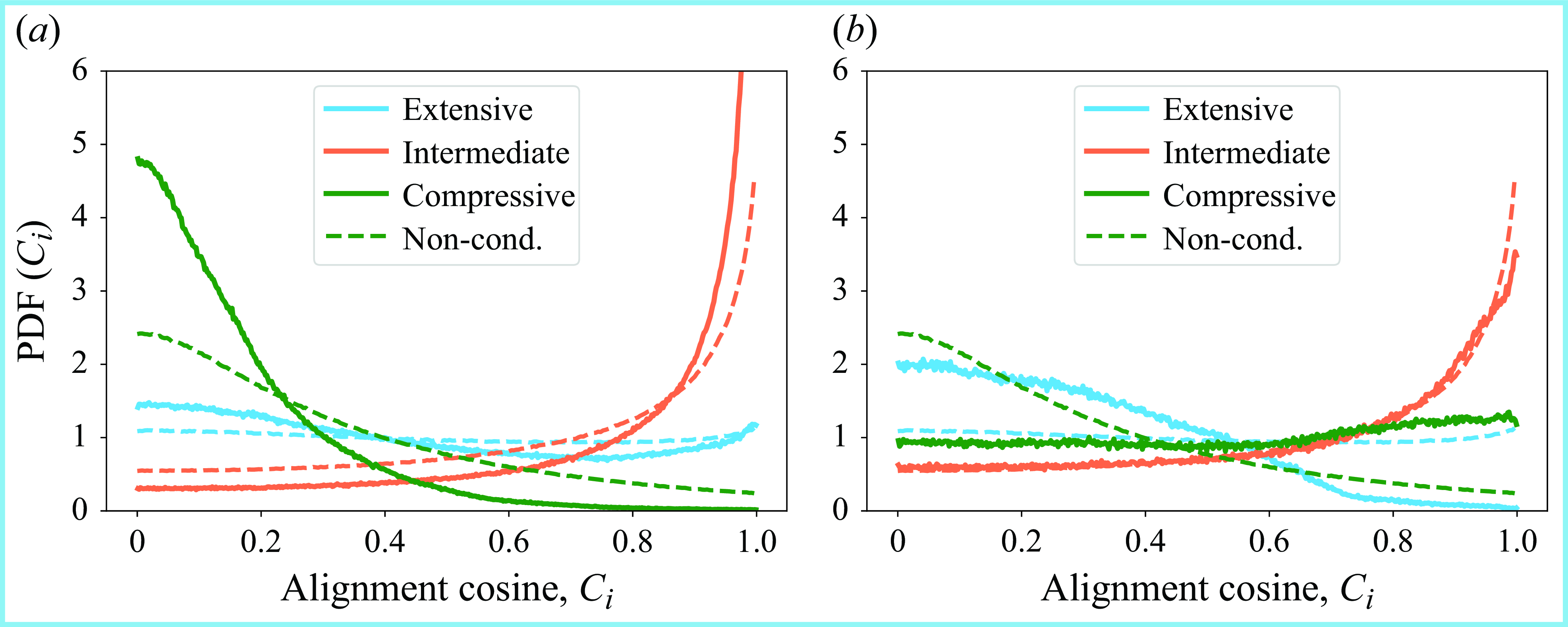
Figure 7. The same as in figure 6, but for
 $Re$
= 39 180,
$Re$
= 39 180,
 $\ell =3.0\, \eta$
.
$\ell =3.0\, \eta$
.
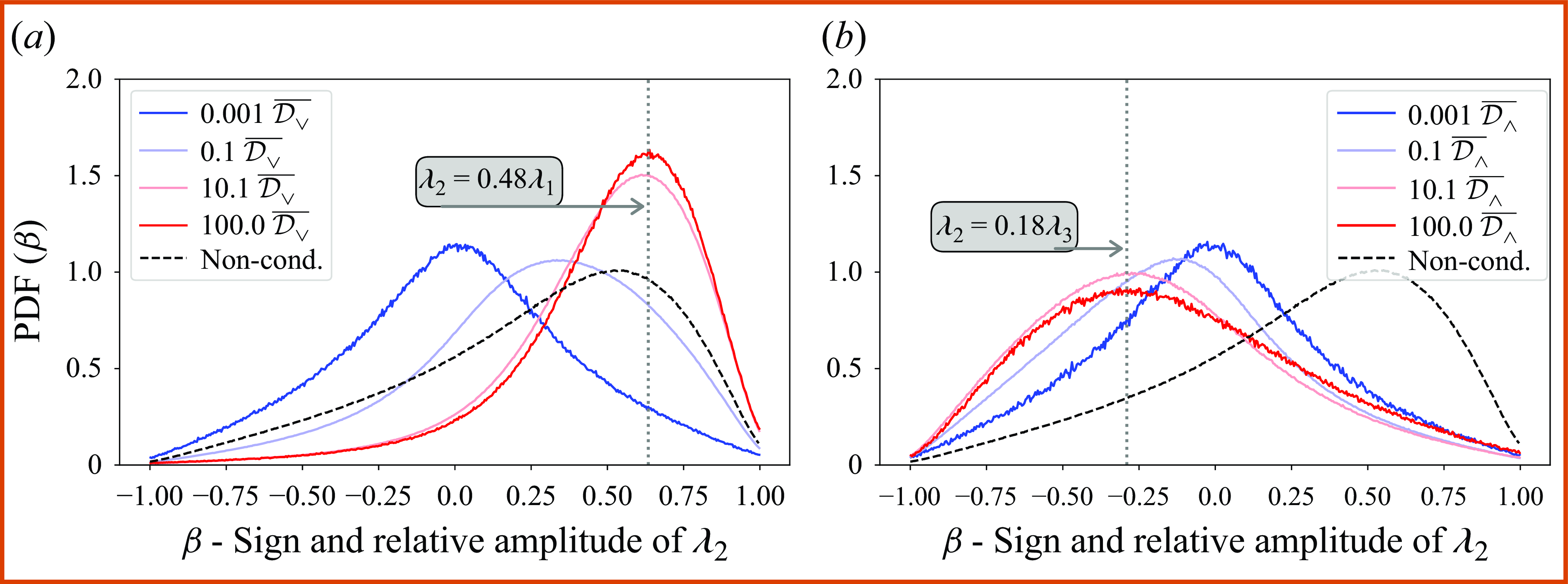
Figure 8. Evolution of the
 $\beta$
distribution when conditioned on varying levels of downscale (a) and upscale (b) energy transfer at
$\beta$
distribution when conditioned on varying levels of downscale (a) and upscale (b) energy transfer at
 $Re$
= 156 719,
$Re$
= 156 719,
 $\ell =6.5\, \eta$
. Conditioning level varies between events of (a) 0.001–100
$\ell =6.5\, \eta$
. Conditioning level varies between events of (a) 0.001–100
 $\overline {\mathcal{D}_{\boldsymbol{\vee }}}$
and (b) 0.001–100
$\overline {\mathcal{D}_{\boldsymbol{\vee }}}$
and (b) 0.001–100
 $\overline {\mathcal{D}_{\boldsymbol{\wedge }}}$
, from smallest (bold blue line) to largest (bold red line). The black dashed line is the non-conditioned result. The value of
$\overline {\mathcal{D}_{\boldsymbol{\wedge }}}$
, from smallest (bold blue line) to largest (bold red line). The black dashed line is the non-conditioned result. The value of
 $\lambda _2 \,$
(relative to
$\lambda _2 \,$
(relative to
 $\lambda _1 \,$
(a) or
$\lambda _1 \,$
(a) or
 $\lambda _3 \,$
(b)) corresponding to the most probable
$\lambda _3 \,$
(b)) corresponding to the most probable
 $\beta$
is shown in the grey text box.
$\beta$
is shown in the grey text box.
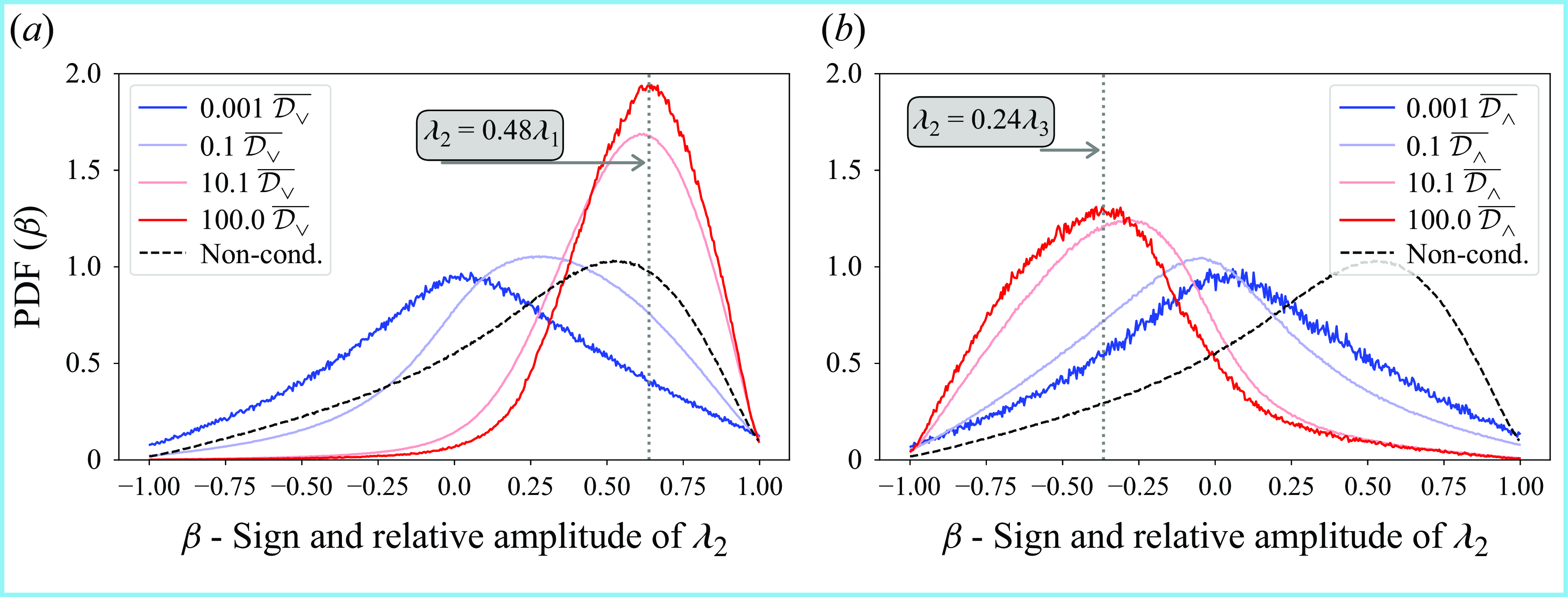
Figure 9. The same as in figure 8, but at
 $Re$
= 39 180,
$Re$
= 39 180,
 $\ell =3.0\eta$
.
$\ell =3.0\eta$
.
Additionally, figures 8(a) and 9(a) show the distribution of
 $\beta$
for a range of conditioning levels, from 0.001 to 100
$\beta$
for a range of conditioning levels, from 0.001 to 100
 $\overline {\mathcal{D}_{\boldsymbol{\vee }}}$
for both
$\overline {\mathcal{D}_{\boldsymbol{\vee }}}$
for both
 $Re$
/scales. The lowest magnitude downscale energy transfer produces a normal-like distribution in
$Re$
/scales. The lowest magnitude downscale energy transfer produces a normal-like distribution in
 $\beta$
with no preference for compressive or extensional
$\beta$
with no preference for compressive or extensional
 $\boldsymbol{e}_2 \,$
. The distribution of
$\boldsymbol{e}_2 \,$
. The distribution of
 $\beta$
gradually shifts rightward as the level of conditioning on
$\beta$
gradually shifts rightward as the level of conditioning on
 $\mathcal{D}_{\boldsymbol{\vee }}$
increases, such that at the largest downscale transfer (
$\mathcal{D}_{\boldsymbol{\vee }}$
increases, such that at the largest downscale transfer (
 ${\gt } 100$
 $\overline {\mathcal{D}_{\boldsymbol{\vee }}}$
)
$\overline {\mathcal{D}_{\boldsymbol{\vee }}}$
)
 $\boldsymbol{e}_2 \,$
is almost entirely extensional. There is also a notable increase in the most probable magnitude relative to
$\boldsymbol{e}_2 \,$
is almost entirely extensional. There is also a notable increase in the most probable magnitude relative to
 $\lambda _1 \,$
(from 0.37
$\lambda _1 \,$
(from 0.37
 $\lambda _1 \,$
to 0.48
$\lambda _1 \,$
to 0.48
 $\lambda _1 \,$
), as indicated by the grey text boxes in figures 3(b), 8(a) and 9(a). When comparing the conditioned
$\lambda _1 \,$
), as indicated by the grey text boxes in figures 3(b), 8(a) and 9(a). When comparing the conditioned
 $\beta$
distributions across scale, we again see that, as we go to smaller scales, the trends are enhanced. That is, for the largest direct cascade events, there is an even greater share of positive
$\beta$
distributions across scale, we again see that, as we go to smaller scales, the trends are enhanced. That is, for the largest direct cascade events, there is an even greater share of positive
 $\beta$
values at
$\beta$
values at
 $\ell = 3.0\eta$
(figure 8
a vs 9
a).
$\ell = 3.0\eta$
(figure 8
a vs 9
a).
The alignment statistics conditioned on upscale energy transfer,
 $\mathcal{D}_{\boldsymbol{\wedge }}$
, are likewise shown in figures 6(b), 7(b), 8(b) and 9(b). The
$\mathcal{D}_{\boldsymbol{\wedge }}$
, are likewise shown in figures 6(b), 7(b), 8(b) and 9(b). The
 $\boldsymbol{\omega }$
–
$\boldsymbol{\omega }$
–
 $\unicode{x1D64E}$
alignments are shown in figures 6(b) and 7(b), where the
$\unicode{x1D64E}$
alignments are shown in figures 6(b) and 7(b), where the
 $\boldsymbol{\omega }$
–
$\boldsymbol{\omega }$
–
 $\boldsymbol{e}_2 \,$
alignment is found to be effectively identical to the non-conditioned case for both scales. However, it notably displays a preference for orthogonality with the extensive
$\boldsymbol{e}_2 \,$
alignment is found to be effectively identical to the non-conditioned case for both scales. However, it notably displays a preference for orthogonality with the extensive
 $\boldsymbol{e}_1 \,$
, instead of the compressive
$\boldsymbol{e}_1 \,$
, instead of the compressive
 $\boldsymbol{e}_3 \,$
as in the non-conditioned case. There seems to be no difference when changing scale in this case, other than small changes likely due to statistical convergence issues.
$\boldsymbol{e}_3 \,$
as in the non-conditioned case. There seems to be no difference when changing scale in this case, other than small changes likely due to statistical convergence issues.
The evolution of the
 $\beta$
distribution is again shown, but for increasing upscale transfers (0.001–100
$\beta$
distribution is again shown, but for increasing upscale transfers (0.001–100
 $\overline {\mathcal{D}_{\boldsymbol{\wedge }}}$
) in figures 8(b) and 9(b). Once again, we note the effectively normal distribution of
$\overline {\mathcal{D}_{\boldsymbol{\wedge }}}$
) in figures 8(b) and 9(b). Once again, we note the effectively normal distribution of
 $\beta$
values for the smallest
$\beta$
values for the smallest
 $\mathcal{D}_{\boldsymbol{\wedge }}$
 $\,$
events. However, as the conditioning level increases, the distribution of
$\,$
events. However, as the conditioning level increases, the distribution of
 $\beta$
moves leftwards to negative values. At the largest upscale energy transfers, for both
$\beta$
moves leftwards to negative values. At the largest upscale energy transfers, for both
 $Re$
/scales,
$Re$
/scales,
 $\beta$
is primarily negative (compressive). However, the larger-scale case (figure 8
b) displays a wider distribution that includes a sizable amount of positive
$\beta$
is primarily negative (compressive). However, the larger-scale case (figure 8
b) displays a wider distribution that includes a sizable amount of positive
 $\lambda _2 \,$
, while for the smaller-scale case (figure 9
b), the trend is enhanced in that
$\lambda _2 \,$
, while for the smaller-scale case (figure 9
b), the trend is enhanced in that
 $\beta$
includes primarily negative values. The relative magnitude of the most probably value of
$\beta$
includes primarily negative values. The relative magnitude of the most probably value of
 $\lambda _2 \,$
as compared with its complimentary eigenvalue (
$\lambda _2 \,$
as compared with its complimentary eigenvalue (
 $\lambda _3 \,$
in this case) has also changed compared with the non-conditioned case – from 0.37
$\lambda _3 \,$
in this case) has also changed compared with the non-conditioned case – from 0.37
 $\lambda _1 \,$
to 0.18
$\lambda _1 \,$
to 0.18
 $\lambda _3 \,$
for the larger
$\lambda _3 \,$
for the larger
 $Re$
/scale, and again further to 0.24
$Re$
/scale, and again further to 0.24
 $\lambda _3 \,$
at the smaller scale.
$\lambda _3 \,$
at the smaller scale.
A notable feature that applies to both the direct and inverse cascade cases, is that
 $\boldsymbol{\omega }$
always shows a preferentially perpendicular alignment with the largest magnitude eigenvector, or the direction of highest amplitude strain. For
$\boldsymbol{\omega }$
always shows a preferentially perpendicular alignment with the largest magnitude eigenvector, or the direction of highest amplitude strain. For
 $\mathcal{D}_{\boldsymbol{\vee }}$
, as
$\mathcal{D}_{\boldsymbol{\vee }}$
, as
 $\lambda _2\;{\gt }\; 0$
,
$\lambda _2\;{\gt }\; 0$
,
 $\boldsymbol{\omega }$
is most perpendicular to
$\boldsymbol{\omega }$
is most perpendicular to
 $\boldsymbol{e}_3 \,$
(because
$\boldsymbol{e}_3 \,$
(because
 $\lambda _1 \,$
+
$\lambda _1 \,$
+
 $\lambda _2 \,$
=
$\lambda _2 \,$
=
 $\lambda _3$
). While for
$\lambda _3$
). While for
 $\,\mathcal{D}_{\boldsymbol{\wedge }}$
,
$\,\mathcal{D}_{\boldsymbol{\wedge }}$
,
 $\boldsymbol{\omega }$
is preferentially orthogonal to
$\boldsymbol{\omega }$
is preferentially orthogonal to
 $\boldsymbol{e}_1 \,$
in the inverse cascade as
$\boldsymbol{e}_1 \,$
in the inverse cascade as
 $\lambda _1 \,$
=
$\lambda _1 \,$
=
 $\lambda _2 \,$
+
$\lambda _2 \,$
+
 $\lambda _3 \,$
.
$\lambda _3 \,$
.
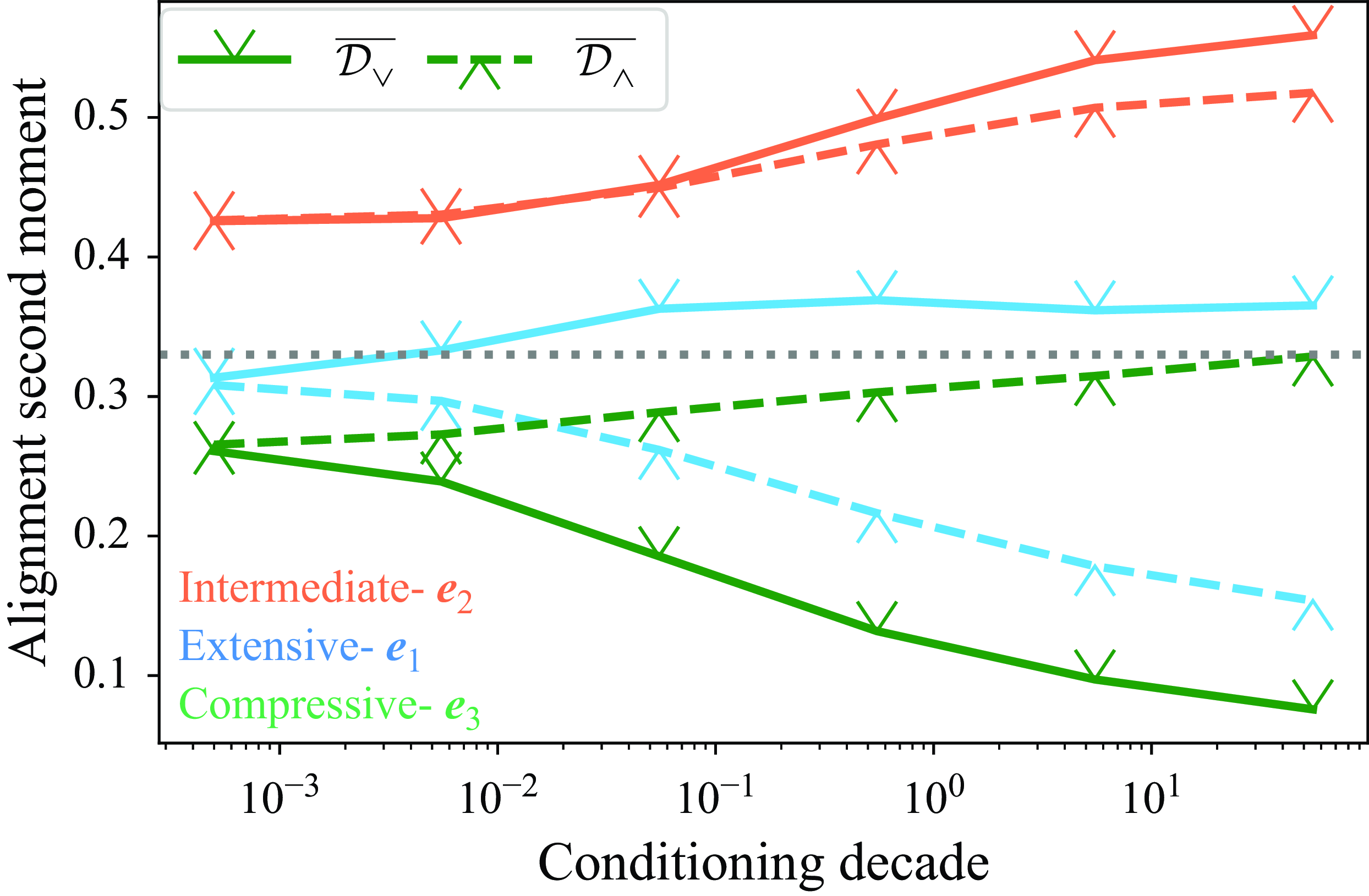
Figure 10. Average second moment of the alignment cosine across a range of increasing amplitude downscale (
 $\overline {\mathcal{D}_{\boldsymbol{\vee }}}$
- solid lines) and upscale (
$\overline {\mathcal{D}_{\boldsymbol{\vee }}}$
- solid lines) and upscale (
 $\overline {\mathcal{D}_{\boldsymbol{\wedge }}}$
- dashed lines) energy transfer conditioning levels. The faint, dotted grey line is at 1/3, which corresponds to uniform distributions of
$\overline {\mathcal{D}_{\boldsymbol{\wedge }}}$
- dashed lines) energy transfer conditioning levels. The faint, dotted grey line is at 1/3, which corresponds to uniform distributions of
 $C_i$
. Values closer to 0 or 1 indicate average perpendicular or parallel
$C_i$
. Values closer to 0 or 1 indicate average perpendicular or parallel
 $\boldsymbol{\omega }$
-
$\boldsymbol{\omega }$
-
 $\boldsymbol{e_i}$
alignment, respectively.
$\boldsymbol{e_i}$
alignment, respectively.
In order to gauge how the alignment might change across different energy amplitudes we investigate the average second moment of the alignment cosine,
 $\langle (\boldsymbol{e}_i \cdot \hat {\boldsymbol{\omega }})^2 \rangle$
. This variable is useful in that it is bounded between 0 and 1, and the sum of the three contributing directions will also sum to 1. The value for each eigenvector gives an idea of the average alignment for the distribution of
$\langle (\boldsymbol{e}_i \cdot \hat {\boldsymbol{\omega }})^2 \rangle$
. This variable is useful in that it is bounded between 0 and 1, and the sum of the three contributing directions will also sum to 1. The value for each eigenvector gives an idea of the average alignment for the distribution of
 $C_i$
at each conditioning level. Its average value conditioned on varying levels of up/downscale energy transfer is shown in figure 10. One can see that, at the highest conditioning levels, we recover the results of figures 6 and 7, where there is greatest preference for
$C_i$
at each conditioning level. Its average value conditioned on varying levels of up/downscale energy transfer is shown in figure 10. One can see that, at the highest conditioning levels, we recover the results of figures 6 and 7, where there is greatest preference for
 $\boldsymbol{\omega }$
-
$\boldsymbol{\omega }$
-
 $\boldsymbol{e}_2 \,$
alignment and a orthogonal preference which swaps between
$\boldsymbol{e}_2 \,$
alignment and a orthogonal preference which swaps between
 $\boldsymbol{e}_3 \,$
for
$\boldsymbol{e}_3 \,$
for
 $\overline {\mathcal{D}_{\boldsymbol{\vee }}}$
events (downscale-solid lines) and
$\overline {\mathcal{D}_{\boldsymbol{\vee }}}$
events (downscale-solid lines) and
 $\boldsymbol{e}_1 \,$
for
$\boldsymbol{e}_1 \,$
for
 $\overline {\mathcal{D}_{\boldsymbol{\wedge }}}$
events (upscale-dashed line). If we note that a eigenvector with no alignment preference (uniformly distributed) will have a value
$\overline {\mathcal{D}_{\boldsymbol{\wedge }}}$
events (upscale-dashed line). If we note that a eigenvector with no alignment preference (uniformly distributed) will have a value
 $\langle (\boldsymbol{e}_i \cdot \hat {\boldsymbol{\omega }})^2 \rangle$
= 1/3 we can make a surprising observation. This is the fact that at the lowest energy transfer levels, the average
$\langle (\boldsymbol{e}_i \cdot \hat {\boldsymbol{\omega }})^2 \rangle$
= 1/3 we can make a surprising observation. This is the fact that at the lowest energy transfer levels, the average
 $\boldsymbol{\omega }$
-
$\boldsymbol{\omega }$
-
 $\unicode{x1D64E}$
alignment seems to maintain a morphological structure. This is surprising as several works have found that
$\unicode{x1D64E}$
alignment seems to maintain a morphological structure. This is surprising as several works have found that
 $\langle (\boldsymbol{e}_i \cdot \hat {\boldsymbol{\omega }})^2 \rangle$
conditioned on the lowest levels of enstrophy or strain will converge to 1/3 for all eigenvectors (Buaria et al. Reference Buaria, Bodenschatz and Pumir2020). This perhaps points to the fact that energy transfer is more inherently linked to morphological structure.
$\langle (\boldsymbol{e}_i \cdot \hat {\boldsymbol{\omega }})^2 \rangle$
conditioned on the lowest levels of enstrophy or strain will converge to 1/3 for all eigenvectors (Buaria et al. Reference Buaria, Bodenschatz and Pumir2020). This perhaps points to the fact that energy transfer is more inherently linked to morphological structure.
We next use the conditioned statistics to generate QR plots for the largest upscale and downscale energy transfer. Figures 11(a) and 12(a) show the QR plots for downscale energy transfers
 ${\gt } 100 \overline {\mathcal{D}_{\boldsymbol{\vee }}}$
 $\,$
at both
$\,$
at both
 $Re$
/scales. While the resulting tear drop is similar to the non-conditioned case, it is considerably more elongated along the Vieillefosse line, especially for the smaller
$Re$
/scales. While the resulting tear drop is similar to the non-conditioned case, it is considerably more elongated along the Vieillefosse line, especially for the smaller
 $Re$
/scale case. Thus, a vast majority of its events are in the VSEP region, where vortex stretching is prominent, and in the sheet forming dissipation-producing regions, SDP. The large downscale energy transfer events also pull the pointed portion of the tear drop further down the right Vieillefosse tail, particularly for the most probable events. In regards to the non-conditioned QR plots the greatest changes are in the SDP region (from non-conditioned to larger scale to smaller scale: 8
$Re$
/scale case. Thus, a vast majority of its events are in the VSEP region, where vortex stretching is prominent, and in the sheet forming dissipation-producing regions, SDP. The large downscale energy transfer events also pull the pointed portion of the tear drop further down the right Vieillefosse tail, particularly for the most probable events. In regards to the non-conditioned QR plots the greatest changes are in the SDP region (from non-conditioned to larger scale to smaller scale: 8
 $\, \%$
to 42
$\, \%$
to 42
 $\, \%$
to 44
$\, \%$
to 44
 $\, \%$
) and the enstrophy-producing non-swirling region (
$\, \%$
) and the enstrophy-producing non-swirling region (
 $48\, \%$
to 7
$48\, \%$
to 7
 $\, \%$
to 6
$\, \%$
to 6
 $\, \%$
).
$\, \%$
).
Alternatively, figures 11(b) and 12(b) shows the QR plots for upscale energy transfers
 ${\gt } 100 \overline {\mathcal{D}_{\boldsymbol{\wedge }}}$
. The tear drop for the inverse cascade is shown beginning to tilt along the opposite Vieillefosse left tail. In this case there are proportionately many more events in the VCDP region, corresponding to vortex-compression topology. Additionally, the most probable events are oriented along the left Vieillefosse tail, a feature that is again enhanced at the smaller scale. In regards to the non-conditioned QR plot the greatest changes occur in the VCDP region (4
${\gt } 100 \overline {\mathcal{D}_{\boldsymbol{\wedge }}}$
. The tear drop for the inverse cascade is shown beginning to tilt along the opposite Vieillefosse left tail. In this case there are proportionately many more events in the VCDP region, corresponding to vortex-compression topology. Additionally, the most probable events are oriented along the left Vieillefosse tail, a feature that is again enhanced at the smaller scale. In regards to the non-conditioned QR plot the greatest changes occur in the VCDP region (4
 $\, \%$
to 49
$\, \%$
to 49
 $\, \%$
to 55
$\, \%$
to 55
 $\, \%$
), the two regions around the right Vieillefosse tail (totals of 15
$\, \%$
), the two regions around the right Vieillefosse tail (totals of 15
 $\, \%$
to 12
$\, \%$
to 12
 $\, \%$
to 6
$\, \%$
to 6
 $\, \%$
) and again in the enstrophy-producing non-swirling region above the left Vieillefosse tail (
$\, \%$
) and again in the enstrophy-producing non-swirling region above the left Vieillefosse tail (
 $48\, \%$
to 8
$48\, \%$
to 8
 $\, \%$
to 11
$\, \%$
to 11
 $\, \%$
). One also observes a large decrease in enstrophy production due to vortex stretching as the smaller scales are reached (VSEP of
$\, \%$
). One also observes a large decrease in enstrophy production due to vortex stretching as the smaller scales are reached (VSEP of
 $28\, \%$
to 20
$28\, \%$
to 20
 $\, \%$
to 11
$\, \%$
to 11
 $\, \%$
). It should be noted that, because net energy transfer is downward, there are fewer statistics for both the inverse cascade as a whole and for large amplitude upscale events, as compared with their downscale counterparts. Thus we have found that the
$\, \%$
). It should be noted that, because net energy transfer is downward, there are fewer statistics for both the inverse cascade as a whole and for large amplitude upscale events, as compared with their downscale counterparts. Thus we have found that the
 $\overline {\mathcal{D}_{\boldsymbol{\vee }}}$
is typically 2.5 times larger than the amplitude of
$\overline {\mathcal{D}_{\boldsymbol{\vee }}}$
is typically 2.5 times larger than the amplitude of
 $\overline {\mathcal{D}_{\boldsymbol{\wedge }}}$
.
$\overline {\mathcal{D}_{\boldsymbol{\wedge }}}$
.
Comparatively, in the downscale case most events are in the regions of enstrophy production via vorticity (VSEP) and dissipation production via strain (SDP). However, in the upscale case, while there is still vortex stretching producing enstrophy, there is also a notable amount of enstrophy production via straining and filaments (FEP). Interestingly, dissipation production is now primarily due to vortex compression (VCDP). Furthermore, as noted previously there exists a much higher degree of nonlinearity in the direct cascade as opposed to the inverse cascade (Tsinober Reference Tsinober1998, Reference Tsinober2009). As these nonlinearities are highly correlated with strain-dominated (
 $2S_{ik}S_{ik} \gt \omega ^2$
), and strain-producing regions (
$2S_{ik}S_{ik} \gt \omega ^2$
), and strain-producing regions (
 $-S_{ik}S_{km}S_{mi} \gt 3/4 \omega _i \omega _k S_{ik}$
) the largest downscale energy transfer may be highly nonlinear due to the preponderance of events along the right tails of figures 11(a) and 12(a).
$-S_{ik}S_{km}S_{mi} \gt 3/4 \omega _i \omega _k S_{ik}$
) the largest downscale energy transfer may be highly nonlinear due to the preponderance of events along the right tails of figures 11(a) and 12(a).
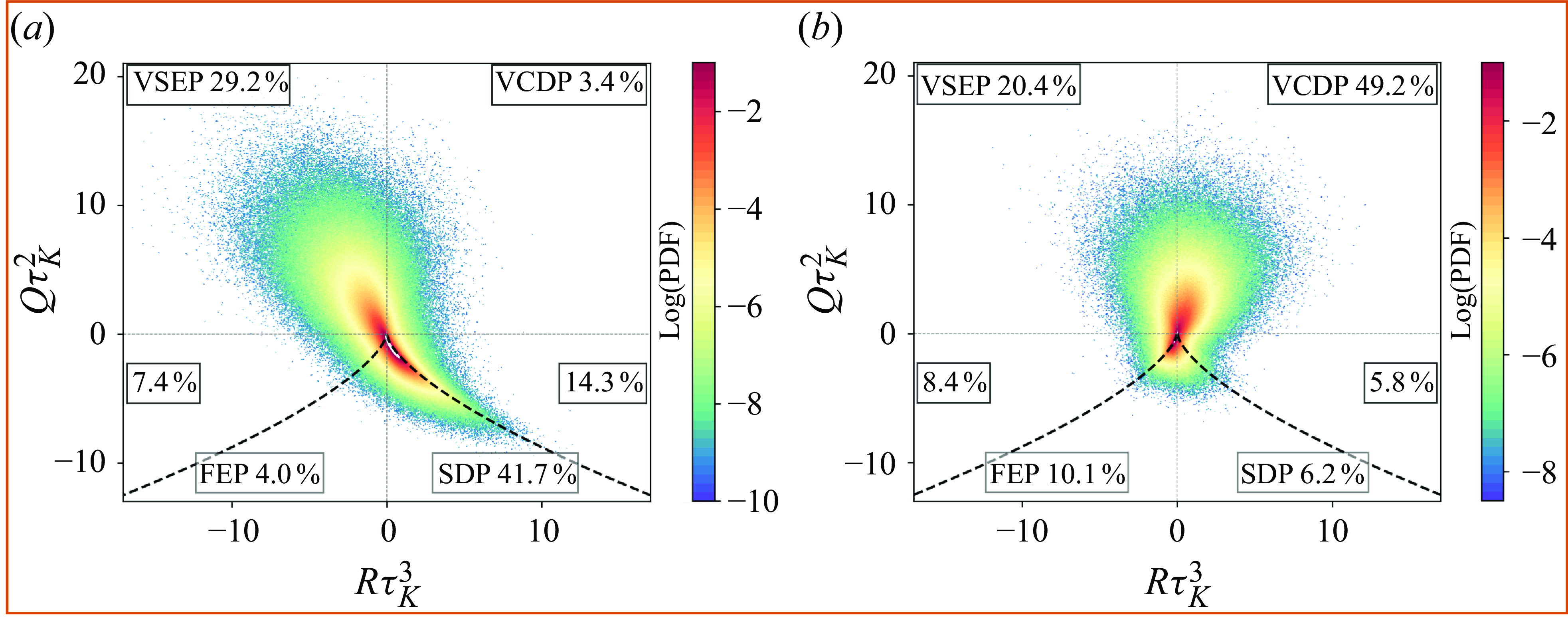
Figure 11. The QR plots conditioned on large magnitude (a) downscale (
 ${\gt } 100 \overline {\mathcal{D}_{\boldsymbol{\vee }}}$
) and (b) upscale (
${\gt } 100 \overline {\mathcal{D}_{\boldsymbol{\vee }}}$
) and (b) upscale (
 ${\gt } 100 \overline {\mathcal{D}_{\boldsymbol{\wedge }}}$
) energy transfer events at
${\gt } 100 \overline {\mathcal{D}_{\boldsymbol{\wedge }}}$
) energy transfer events at
 $Re$
= 156 719,
$Re$
= 156 719,
 $\ell =6.5\, \eta$
. The percentage of events located in each labelled region (acronyms defined previously in the text and figure 4) are indicated in the text boxes. The dashed line is the Vieillefosse line. The plots have been non-dimensionalised using the appropriate powers of
$\ell =6.5\, \eta$
. The percentage of events located in each labelled region (acronyms defined previously in the text and figure 4) are indicated in the text boxes. The dashed line is the Vieillefosse line. The plots have been non-dimensionalised using the appropriate powers of
 $\tau _{K}$
.
$\tau _{K}$
.

Figure 12. The same as in figure 11, but at
 $Re$
= 39 180,
$Re$
= 39 180,
 $\ell =3.0\eta$
.
$\ell =3.0\eta$
.
4.3. Contribution of individual eigenvectors
Understanding the amplitude and direction of each eigenvector is crucial for delineating the contributions of vortex stretching and strain-rate to large amplitude energy transfer. These contributions can be better understood by examining the governing equations for the enstrophy,
 $\Omega$
, and an estimate of the dissipation rate,
$\Omega$
, and an estimate of the dissipation rate,
 $\Sigma$
, (where
$\Sigma$
, (where
 $\Sigma = 2 S_{ij}S_{ij}$
and the local dissipation rate is
$\Sigma = 2 S_{ij}S_{ij}$
and the local dissipation rate is
 $\epsilon = \nu \Sigma$
), both shown here
$\epsilon = \nu \Sigma$
), both shown here
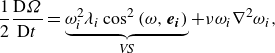 \begin{align} \frac {1}{2} \frac {{\rm D}\Omega }{{\rm D}t} & = \underbrace {\omega _i^2 \lambda _i \cos ^2{(\omega ,\boldsymbol{e_i})}}_{\textit{VS}} + \nu \omega _i \nabla ^2 \omega _i ,\end{align}
 \begin{align} \frac {1}{2}\frac {{\rm D} \Sigma }{{\rm D}t} & = -\underbrace {(\lambda _1^3 +\lambda _2^3 +\lambda _3^3)}_{\textit{SSA}} - \frac {1}{4} \underbrace {\omega _i^2 \lambda _i \cos ^2{(\omega ,\boldsymbol{e_i})}}_{\textit{VS}} - S_{ij} \frac {\partial ^2 p} {\partial x_i \partial x_j} + \nu S_{ij} \nabla ^2 S_{ij} .\end{align}
Above, we have neglected external forcing and replaced the vortex-stretching (VS =
 $\omega _i \omega _j S_{ij}$
) and strain-self-amplification terms (SSA =
$\omega _i \omega _j S_{ij}$
) and strain-self-amplification terms (SSA =
 $S_{ij}S_{jk}S_{ki}$
) with equivalent terms based on the eigenvalues of
$S_{ij}S_{jk}S_{ki}$
) with equivalent terms based on the eigenvalues of
 $\unicode{x1D64E}$
(Tsinober Reference Tsinober2009; Buaria & Pumir Reference Buaria and Pumir2021).
$\unicode{x1D64E}$
(Tsinober Reference Tsinober2009; Buaria & Pumir Reference Buaria and Pumir2021).
From (4.1) we can see that only the first term on the right-hand side (the vortex-stretching term) is a source of
 $\Omega$
production, and this is only the case when
$\Omega$
production, and this is only the case when
 $\lambda _i \gt 0$
. Additionally, the contribution from each eigenvector depends on both the alignment and the magnitude. The vortex-stretching (VS) term also occurs in (4.2) as a sink, albeit with three quarters less effect. Thus, in this case when
$\lambda _i \gt 0$
. Additionally, the contribution from each eigenvector depends on both the alignment and the magnitude. The vortex-stretching (VS) term also occurs in (4.2) as a sink, albeit with three quarters less effect. Thus, in this case when
 $\lambda _i \gt 0$
, the VS term opposes dissipation production, while it creates dissipation when
$\lambda _i \gt 0$
, the VS term opposes dissipation production, while it creates dissipation when
 $\lambda _i \lt 0$
.
$\lambda _i \lt 0$
.
Alternatively, the first term on the right-hand side of (4.2) is the strain-self-amplification term, which produces dissipation only if two eigenvalues are positive. This has two important implications, the first being that due to incompressibility
 $\lambda _1 \,$
+
$\lambda _1 \,$
+
 $\lambda _2 \,$
+
$\lambda _2 \,$
+
 $\lambda _3 \,$
= 0, and in the situation where
$\lambda _3 \,$
= 0, and in the situation where
 $\lambda _1 \,$
,
$\lambda _1 \,$
,
 $\lambda _2 \;\gt\; 0$
, the only term contributing to the production of dissipation through SSA is the compressive strain eigenvector
$\lambda _2 \;\gt\; 0$
, the only term contributing to the production of dissipation through SSA is the compressive strain eigenvector
 $\boldsymbol{e}_3 \,$
(Gulitski et al. Reference Gulitski, Kholmyansky, Kinzelbach, Lüthi, Tsinober and Yorish2007). One should also note that, in this case (
$\boldsymbol{e}_3 \,$
(Gulitski et al. Reference Gulitski, Kholmyansky, Kinzelbach, Lüthi, Tsinober and Yorish2007). One should also note that, in this case (
 $\lambda _2 \, {\gt } 0$
), the larger the magnitude of
$\lambda _2 \, {\gt } 0$
), the larger the magnitude of
 $\lambda _2 \,$
, the larger the SSA, as
$\lambda _2 \,$
, the larger the SSA, as
 $\lambda _1 \, \approx \lambda _2 \,$
minimises their respective negative contributions, due to the cubed powers in (4.2). Second, it is not possible to produce dissipation through the SSA term when
$\lambda _1 \, \approx \lambda _2 \,$
minimises their respective negative contributions, due to the cubed powers in (4.2). Second, it is not possible to produce dissipation through the SSA term when
 $\lambda _2 \;\lt\; 0$
as only two positive eigenvalues yield a positive number, and by definition
$\lambda _2 \;\lt\; 0$
as only two positive eigenvalues yield a positive number, and by definition
 $\lambda _1 \;\gt\; 0$
and
$\lambda _1 \;\gt\; 0$
and
 $\lambda _3 \;\lt\; 0$
. This can be observed in our data in figure 13, as the SSA term conditioned on the inverse cascade (SSA
$\lambda _3 \;\lt\; 0$
. This can be observed in our data in figure 13, as the SSA term conditioned on the inverse cascade (SSA
 $| \overline {\mathcal{D}_{\boldsymbol{\wedge }}}$
) begins to destroy dissipation once the upscale energy amplitude reaches a level where the distribution of
$| \overline {\mathcal{D}_{\boldsymbol{\wedge }}}$
) begins to destroy dissipation once the upscale energy amplitude reaches a level where the distribution of
 $\lambda _2 \,$
skews negative (see
$\lambda _2 \,$
skews negative (see
 $\beta$
in figures 8
b, 9
b). This fact demonstrates that the compressive action of
$\beta$
in figures 8
b, 9
b). This fact demonstrates that the compressive action of
 $\boldsymbol{e}_3 \,$
alone is what skews
$\boldsymbol{e}_3 \,$
alone is what skews
 $\langle S_{ij}S_{jk}S_{ki}\rangle$
negative, and because this term is proportional to the distribution of velocity derivatives, it’s also responsible for their negative skewness. In other words, the compression of
$\langle S_{ij}S_{jk}S_{ki}\rangle$
negative, and because this term is proportional to the distribution of velocity derivatives, it’s also responsible for their negative skewness. In other words, the compression of
 $\boldsymbol{e}_3 \,$
results in the negative skewness of longitudinal velocity increments, a hallmark of the intrinsic non-Gaussian structure of turbulent statistics, and an exact result of the Kolmogorov 4/5th law (Rosales & Meneveau Reference Rosales and Meneveau2006). This suggests that, because we observe a generally negative
$\boldsymbol{e}_3 \,$
results in the negative skewness of longitudinal velocity increments, a hallmark of the intrinsic non-Gaussian structure of turbulent statistics, and an exact result of the Kolmogorov 4/5th law (Rosales & Meneveau Reference Rosales and Meneveau2006). This suggests that, because we observe a generally negative
 $\lambda _2 \,$
(figures 8
b and 9
b) in the inverse cascade case, longitudinal velocity increments should skew less negatively for large upscale energy transfer.
$\lambda _2 \,$
(figures 8
b and 9
b) in the inverse cascade case, longitudinal velocity increments should skew less negatively for large upscale energy transfer.

Figure 13. Average VS (in (4.1)) and strain-self-amplification (SSA in (4.2)) terms conditioned on increasing amplitudes of direct (
 $\overline {\mathcal{D}_{\boldsymbol{\vee }}}$
– orange hues) and inverse (
$\overline {\mathcal{D}_{\boldsymbol{\vee }}}$
– orange hues) and inverse (
 $\overline {\mathcal{D}_{\boldsymbol{\wedge }}}$
– green hues) cascade events. Dashed portions of the lines represent destruction of the respective quantity. Pale hues show VS, while deeper colours are SSA.
$\overline {\mathcal{D}_{\boldsymbol{\wedge }}}$
– green hues) cascade events. Dashed portions of the lines represent destruction of the respective quantity. Pale hues show VS, while deeper colours are SSA.
The average values of the VS and SSA terms in (4.1) and (4.2) are shown for different levels of direct and inverse cascade conditioning in figure 13. For the direct cascade case, both VS and SSA increase as a power law dependent on the energy transfer amplitude. However, in the case of inverse cascade, these terms both decrease as upscale amplitude increases, until the point where they actually become net sinks of enstrophy and dissipation (as indicated by the dotted lines in figure 13). Note that in this analysis we have neglected the pressure Hessian term (the third component on the right-hand side of (4.2)) as we are not able to measure pressure. This non-local term is also neglected in the restricted Euler formulation, and as such is thought to play a role in preventing finite time singularities (Chevillard et al. Reference Chevillard, Meneveau, Biferale and Toschi2008; Wilczek & Meneveau Reference Wilczek and Meneveau2014).
Understanding the contributions to the VS term is more complicated due to the simultaneous dependence on alignment, sign and amplitude. Thus we show the average individual contributions of each eigenvector to enstrophy production via the normalised VS term in figure 14. One can see that in the direct cascade case of figure 14(a), the
 $\boldsymbol{e}_2 \,$
contribution grows steadily with increasing energy transfer amplitude until the largest events where it nearly matches the contribution from
$\boldsymbol{e}_2 \,$
contribution grows steadily with increasing energy transfer amplitude until the largest events where it nearly matches the contribution from
 $\boldsymbol{e}_1 \,$
. Notably,
$\boldsymbol{e}_1 \,$
. Notably,
 $\boldsymbol{e}_1 \,$
is shown to still contribute majorly despite the preference of
$\boldsymbol{e}_1 \,$
is shown to still contribute majorly despite the preference of
 $\boldsymbol{\omega }$
-
$\boldsymbol{\omega }$
-
 $\boldsymbol{e}_2 \,$
alignment, at least in the average sense.
$\boldsymbol{e}_2 \,$
alignment, at least in the average sense.

Figure 14. Normalised contributions of each
 $\unicode{x1D64E}$
eigenvector towards the VS term in (4.1) conditioned on increasing amplitudes of (a)
$\unicode{x1D64E}$
eigenvector towards the VS term in (4.1) conditioned on increasing amplitudes of (a)
 $\overline {\mathcal{D}_{\boldsymbol{\vee }}}$
– downscale and (b)
$\overline {\mathcal{D}_{\boldsymbol{\vee }}}$
– downscale and (b)
 $\overline {\mathcal{D}_{\boldsymbol{\wedge }}}$
– upscale energy transfer. The bars shown are all the same normalised height, and the size/contribution of each eigenvector is found by dividing the absolute value of the eigenvalue contribution by the absolute value sum of all the contributions. The eigenvalue contributions which contribute negatively are shown below the dashed line at 0 on the
$\overline {\mathcal{D}_{\boldsymbol{\wedge }}}$
– upscale energy transfer. The bars shown are all the same normalised height, and the size/contribution of each eigenvector is found by dividing the absolute value of the eigenvalue contribution by the absolute value sum of all the contributions. The eigenvalue contributions which contribute negatively are shown below the dashed line at 0 on the
 $y$
axis. The white dot signifies the net normalised sum of the contributions.
$y$
axis. The white dot signifies the net normalised sum of the contributions.
Concerning the inverse cascade (figure 14
b), we see that once the mean conditioning level is reached, there is actually a net destruction of enstrophy due to VS (as the negative contributions crosses the white
 $50\, \%$
line). Further, the relative contribution of
$50\, \%$
line). Further, the relative contribution of
 $\boldsymbol{e}_2 \,$
remains small for all conditioning levels and the VS term in the inverse cascade is dominated by the most extensive and compressive eigenvectors, despite the preference for
$\boldsymbol{e}_2 \,$
remains small for all conditioning levels and the VS term in the inverse cascade is dominated by the most extensive and compressive eigenvectors, despite the preference for
 $\boldsymbol{\omega }$
-
$\boldsymbol{\omega }$
-
 $\boldsymbol{e}_2 \,$
alignment.
$\boldsymbol{e}_2 \,$
alignment.
5. Discussion
5.1. Importance of strain vs. Vortex stretching
If we return to the conditioned
 $\beta$
statistics (figures 8 and 9), during the largest direct cascade events the relative magnitude of
$\beta$
statistics (figures 8 and 9), during the largest direct cascade events the relative magnitude of
 $\lambda _2 \,$
increases from 37
$\lambda _2 \,$
increases from 37
 $\, \%$
of
$\, \%$
of
 $\lambda _1 \,$
in the non-conditioned statistics to nearly 50
$\lambda _1 \,$
in the non-conditioned statistics to nearly 50
 $\, \%$
for both
$\, \%$
for both
 $Re$
/scales. Coupled with the stronger degree of
$Re$
/scales. Coupled with the stronger degree of
 $\boldsymbol{\omega }$
-
$\boldsymbol{\omega }$
-
 $\boldsymbol{e}_2 \,$
alignment, especially at the smallest scale, this indicates a very large contribution from
$\boldsymbol{e}_2 \,$
alignment, especially at the smallest scale, this indicates a very large contribution from
 $\boldsymbol{e}_2 \,$
to the velocity-gradient dynamics, as we have already remarked in figure 14(a). One can also see the near total absence of negative (compressive)
$\boldsymbol{e}_2 \,$
to the velocity-gradient dynamics, as we have already remarked in figure 14(a). One can also see the near total absence of negative (compressive)
 $\lambda _2 \,$
for the largest direct cascade events (figures 8
a and 9
a), which can also be observed in the corresponding QR plots of figure 11(a) and 12(a). Notably, both trends seems to strengthen as our scale approaches
$\lambda _2 \,$
for the largest direct cascade events (figures 8
a and 9
a), which can also be observed in the corresponding QR plots of figure 11(a) and 12(a). Notably, both trends seems to strengthen as our scale approaches
 $\eta$
. This manifests such that there are merely 1 %–3
$\eta$
. This manifests such that there are merely 1 %–3
 $\, \%$
of all events located in the vortex-compressing region VCDP. Additionally, simultaneous
$\, \%$
of all events located in the vortex-compressing region VCDP. Additionally, simultaneous
 $\boldsymbol{\omega }$
alignment with
$\boldsymbol{\omega }$
alignment with
 $\boldsymbol{e}_2 \,$
and orthogonality with a large magnitude compressive
$\boldsymbol{e}_2 \,$
and orthogonality with a large magnitude compressive
 $\boldsymbol{e}_3 \,$
indicates morphology that is more akin to strain self-amplification (i.e. figure 1
b) than VS. This is indeed observed in the QR plot as nearly 50
$\boldsymbol{e}_3 \,$
indicates morphology that is more akin to strain self-amplification (i.e. figure 1
b) than VS. This is indeed observed in the QR plot as nearly 50
 $\, \%$
of events are found along the right Vieillefosse tail for both
$\, \%$
of events are found along the right Vieillefosse tail for both
 $Re$
/scales.
$Re$
/scales.
In figures 8(b) and 9(b), for the largest inverse cascade events,
 $\beta$
has the reverse trend, where the relative amplitude of
$\beta$
has the reverse trend, where the relative amplitude of
 $\lambda _2 \,$
decreases from 37
$\lambda _2 \,$
decreases from 37
 $\, \%$
of
$\, \%$
of
 $\lambda _1 \,$
to 18 %–24
$\lambda _1 \,$
to 18 %–24
 $\, \%$
of
$\, \%$
of
 $\lambda _3 \,$
. This means that for the largest upscale events the compressive and extensive eigenvectors have large relative amplitudes and dominate the strain magnitude, despite the persistence of
$\lambda _3 \,$
. This means that for the largest upscale events the compressive and extensive eigenvectors have large relative amplitudes and dominate the strain magnitude, despite the persistence of
 $\boldsymbol{\omega }$
-
$\boldsymbol{\omega }$
-
 $\boldsymbol{e}_2 \,$
alignment. One can see the link between the inverse cascade QR plots (figures 11
b and 12
b) and figures 8(b) and 9(b) by noting the relatively wide distribution of
$\boldsymbol{e}_2 \,$
alignment. One can see the link between the inverse cascade QR plots (figures 11
b and 12
b) and figures 8(b) and 9(b) by noting the relatively wide distribution of
 $\beta$
during the largest events. Because there is a large number of positive and negative values of
$\beta$
during the largest events. Because there is a large number of positive and negative values of
 $\lambda _2 \,$
, this manifests in the QR plot as a plethora of events in both the vortex-stretching (VSEP) and compressing (VCDP) regions. However, at the smallest scale we see this effect diminish, as the strongly peaked
$\lambda _2 \,$
, this manifests in the QR plot as a plethora of events in both the vortex-stretching (VSEP) and compressing (VCDP) regions. However, at the smallest scale we see this effect diminish, as the strongly peaked
 $\beta$
distribution in figure 9(b) shows very few positive
$\beta$
distribution in figure 9(b) shows very few positive
 $\lambda _2 \,$
values while figure 12(b) simultaneously shows a halving of the amount of events located in the VSEP region.
$\lambda _2 \,$
values while figure 12(b) simultaneously shows a halving of the amount of events located in the VSEP region.
Therefore we posit that, at larger scales, because there is a comparable number of VS topologies in the VSEP region for both the direct (29
 $\, \%$
in figure 11
a) and inverse (20
$\, \%$
in figure 11
a) and inverse (20
 $\, \%$
in figure 11
b) cascade, VS is perhaps not the primary factor in determining cascade direction. Although as mentioned, VS topologies may be capable of serving as a diagnostic for cascade direction at scales closer to
$\, \%$
in figure 11
b) cascade, VS is perhaps not the primary factor in determining cascade direction. Although as mentioned, VS topologies may be capable of serving as a diagnostic for cascade direction at scales closer to
 $\eta$
. However, for both
$\eta$
. However, for both
 $Re$
/scales, it is the number of vortex-compressing events (only 3 %–1
$Re$
/scales, it is the number of vortex-compressing events (only 3 %–1
 $\, \%$
in downscale vs 49 %–55
$\, \%$
in downscale vs 49 %–55
 $\, \%$
in upscale) and strain-self-amplification events (over 50
$\, \%$
in upscale) and strain-self-amplification events (over 50
 $\, \%$
for both scales in direct cascade and under 10
$\, \%$
for both scales in direct cascade and under 10
 $\, \%$
in inverse cascade) that mark the key phenomenological differences in cascade direction. Additionally, one can see the most probable values of the large amplitude inverse cascade beginning to orient along the left Vieillefosse tail in figures 11(b) and 12(b).
$\, \%$
in inverse cascade) that mark the key phenomenological differences in cascade direction. Additionally, one can see the most probable values of the large amplitude inverse cascade beginning to orient along the left Vieillefosse tail in figures 11(b) and 12(b).
More generally, these results seem to add credence to the idea that the role of vorticity in the energy cascade is overblown (Tsinober Reference Tsinober1998; Carbone & Bragg Reference Carbone and Bragg2020; Johnson Reference Johnson2020; Vela-Martín & Jiménez Reference Vela-Martín and Jiménez2021). The most obvious sign of this is seen in figures 11 and 12, as was just discussed above. The eigenvector directionality for the inverse (
 $\lambda _3$
,
$\lambda _3$
,
 $\lambda _2 \;\lt\; 0$
) and direct (
$\lambda _2 \;\lt\; 0$
) and direct (
 $\lambda _1 $
,
$\lambda _1 $
,
 $\lambda _2 \;\gt \; 0$
) cascades found in this work also agree with that found in Vela-Martín & Jiménez (Reference Vela-Martín and Jiménez2021). This result shows that downscale energy transfer is much more likely to have self-strain amplification due to its single negative eigenvector. With our scale comparison showing that the likelihood of SSA should increase for large direct cascade events at scales closer to
$\lambda _2 \;\gt \; 0$
) cascades found in this work also agree with that found in Vela-Martín & Jiménez (Reference Vela-Martín and Jiménez2021). This result shows that downscale energy transfer is much more likely to have self-strain amplification due to its single negative eigenvector. With our scale comparison showing that the likelihood of SSA should increase for large direct cascade events at scales closer to
 $\eta$
. While the largest upscale energy transfer events show a repulsion for straining topologies – for both
$\eta$
. While the largest upscale energy transfer events show a repulsion for straining topologies – for both
 $Re$
/scales only approximately
$Re$
/scales only approximately
 $15\, \%$
of all events exist below the Vieillefosse lines in figures 11(b) and 12(b). However, a notable departure between this work and that of Vela-Martín & Jiménez (Reference Vela-Martín and Jiménez2021) is our observation that the number of vortex-compressing events varies drastically between the large amplitude direct and inverse cascade. The aforementioned numerical work (large eddy simulation) showed vortex compression to exist in large quantities for both directions. We posit that this difference is primarily due to two factors, the first being that our statistics concern scales (6.5
$15\, \%$
of all events exist below the Vieillefosse lines in figures 11(b) and 12(b). However, a notable departure between this work and that of Vela-Martín & Jiménez (Reference Vela-Martín and Jiménez2021) is our observation that the number of vortex-compressing events varies drastically between the large amplitude direct and inverse cascade. The aforementioned numerical work (large eddy simulation) showed vortex compression to exist in large quantities for both directions. We posit that this difference is primarily due to two factors, the first being that our statistics concern scales (6.5
 $\eta$
–3.0
$\eta$
–3.0
 $\eta$
) much smaller than the large scales explicitly resolved in their work. Additionally the departure from their results increases for our smallest-scale results, strengthening this argument. Second, our statistics are conditioned on the largest energy transfer events, whereas their work artificially forced the average flow of energy to be up or down scale.
$\eta$
) much smaller than the large scales explicitly resolved in their work. Additionally the departure from their results increases for our smallest-scale results, strengthening this argument. Second, our statistics are conditioned on the largest energy transfer events, whereas their work artificially forced the average flow of energy to be up or down scale.
5.2. Morphology and singularity aspects
Recalling aspects of the discussion above can give us an idea on the vortex morphology during large amplitude energy transfer events. Considering that during the largest downscale events, we observe (i) high positivity of
 $\lambda _2 \,$
, (ii) relatively large magnitude
$\lambda _2 \,$
, (ii) relatively large magnitude
 $\lambda _2 \,$
as compared with
$\lambda _2 \,$
as compared with
 $\lambda _1 \,$
and (iii) a strong preference for orthogonality between
$\lambda _1 \,$
and (iii) a strong preference for orthogonality between
 $\boldsymbol{\omega }$
and
$\boldsymbol{\omega }$
and
 $\boldsymbol{e}_3 \,$
we see a mechanism for the formation of sheet-like structures. Noting, of course, that our results show this mechanism to be enhanced for scales closer to
$\boldsymbol{e}_3 \,$
we see a mechanism for the formation of sheet-like structures. Noting, of course, that our results show this mechanism to be enhanced for scales closer to
 $\eta$
. The vortex, being well aligned with a large amplitude
$\eta$
. The vortex, being well aligned with a large amplitude
 $\boldsymbol{e}_2 \,$
, is compressed strongly by the largest amplitude eigenvector
$\boldsymbol{e}_2 \,$
, is compressed strongly by the largest amplitude eigenvector
 $\boldsymbol{e}_3 \,$
, and simultaneously pulled strongly by
$\boldsymbol{e}_3 \,$
, and simultaneously pulled strongly by
 $\boldsymbol{e}_2 \,$
and
$\boldsymbol{e}_2 \,$
and
 $\boldsymbol{e}_1 \,$
. This bi-axial straining configuration has been observed to be responsible for the maintenance of intense shear layers in turbulent flows (Watanabe, Tanaka & Nagata Reference Watanabe, Tanaka and Nagata2020), while other works (Arun & Colonius Reference Arun and Colonius2024) have found extreme velocity gradients to be most associated with pure shearing regions of the flow. This straining mechanism, illustrated in figure 1(b), is associated with the squeezing of fluid elements into sheet-like structures and has been observed in previous works in flow regions with high vorticity (Vincent & Meneguzzi Reference Vincent and Meneguzzi1994; Rosales & Meneveau Reference Rosales and Meneveau2006). The formation of these sheets can then induce shearing instabilities that in turn cause roll-up of the compressed vortex sheets. In fact this has been found to be the case using the triple decomposition of the velocity-gradient tensor in previous works, which have shown that the generation of vortex tubes is due to the Kelvin–Helmholtz instability acting on vortex sheets, or layers of intense shear (Watanabe et al. Reference Watanabe, Tanaka and Nagata2020). The fact that the most populous region of the QR plot in this work is along the Vieillefosse right tail perhaps signals that quasi-singularities may be associated with vortex-sheet morphology and pure shearing motions more so than those of vortex tubes supports recent works which have come to similar conclusions (Watanabe et al. Reference Watanabe, Tanaka and Nagata2020; Nagata et al. Reference Nagata, Watanabe, Nagata and da Silva2020; Arun & Colonius Reference Arun and Colonius2024.
$\boldsymbol{e}_1 \,$
. This bi-axial straining configuration has been observed to be responsible for the maintenance of intense shear layers in turbulent flows (Watanabe, Tanaka & Nagata Reference Watanabe, Tanaka and Nagata2020), while other works (Arun & Colonius Reference Arun and Colonius2024) have found extreme velocity gradients to be most associated with pure shearing regions of the flow. This straining mechanism, illustrated in figure 1(b), is associated with the squeezing of fluid elements into sheet-like structures and has been observed in previous works in flow regions with high vorticity (Vincent & Meneguzzi Reference Vincent and Meneguzzi1994; Rosales & Meneveau Reference Rosales and Meneveau2006). The formation of these sheets can then induce shearing instabilities that in turn cause roll-up of the compressed vortex sheets. In fact this has been found to be the case using the triple decomposition of the velocity-gradient tensor in previous works, which have shown that the generation of vortex tubes is due to the Kelvin–Helmholtz instability acting on vortex sheets, or layers of intense shear (Watanabe et al. Reference Watanabe, Tanaka and Nagata2020). The fact that the most populous region of the QR plot in this work is along the Vieillefosse right tail perhaps signals that quasi-singularities may be associated with vortex-sheet morphology and pure shearing motions more so than those of vortex tubes supports recent works which have come to similar conclusions (Watanabe et al. Reference Watanabe, Tanaka and Nagata2020; Nagata et al. Reference Nagata, Watanabe, Nagata and da Silva2020; Arun & Colonius Reference Arun and Colonius2024.
More generally, our work supports the ideas that for extreme events in downscale inter-scale energy transfer are associated with coherent structures. This is true at least compared with the unconditioned case, as the alignments of
 $C_i$
show a preference for more enhanced alignment with
$C_i$
show a preference for more enhanced alignment with
 $\boldsymbol{\omega }$
. These findings support previous works which demonstrated that a handful of large magnitude
$\boldsymbol{\omega }$
. These findings support previous works which demonstrated that a handful of large magnitude
 $\mathcal{D}_{\boldsymbol{\vee }}$
 $\,$
events were located within coherent flow structures (Saw et al. Reference Saw, Kuzzay, Faranda, Guittonneau, Daviaud, Wiertel-Gasquet, Padilla and Dubrulle2016; Debue et al. Reference Debue, Shukla, Kuzzay, Faranda, Saw, Daviaud and Dubrulle2018b
, Reference Debue, Valori, Cuvier, Daviaud, Foucaut, Laval, Wiertel, Padilla and Dubrulle2021). Coherent structures, which we can now show to exchange large amounts of energy at least down to
$\,$
events were located within coherent flow structures (Saw et al. Reference Saw, Kuzzay, Faranda, Guittonneau, Daviaud, Wiertel-Gasquet, Padilla and Dubrulle2016; Debue et al. Reference Debue, Shukla, Kuzzay, Faranda, Saw, Daviaud and Dubrulle2018b
, Reference Debue, Valori, Cuvier, Daviaud, Foucaut, Laval, Wiertel, Padilla and Dubrulle2021). Coherent structures, which we can now show to exchange large amounts of energy at least down to
 $3\eta$
. Conversely, while we cannot say the alignment is enhanced for cases of extreme upscale energy transfer, we can at least state that if this is associated with coherent structures, they will be different than those occurring during the direct cascade. However, the previously established link between
$3\eta$
. Conversely, while we cannot say the alignment is enhanced for cases of extreme upscale energy transfer, we can at least state that if this is associated with coherent structures, they will be different than those occurring during the direct cascade. However, the previously established link between
 $\mathcal{D}_\ell$
and regions of the flow with either low dissipation or high intermittency, allow us to in turn associate the morphologies (for extremes in both
$\mathcal{D}_\ell$
and regions of the flow with either low dissipation or high intermittency, allow us to in turn associate the morphologies (for extremes in both
 $\mathcal{D}_{\boldsymbol{\wedge }}$
and
$\mathcal{D}_{\boldsymbol{\wedge }}$
and
 $\mathcal{D}_{\boldsymbol{\vee }}$
) found in this work with those phenomena.
$\mathcal{D}_{\boldsymbol{\vee }}$
) found in this work with those phenomena.
We must also consider that this dominant alignment in the direct cascade case was shown by Vieillefosse (Reference Vieillefosse1982), Cantwell (Reference Cantwell1992) to cause restricted Euler singularities in the velocity gradient along the right Vieillefosse tail. Notably, we not only see this form accentuated for the largest downscale energy transfer events, but also an elongation of the tear-drop shape along the right Vieillefosse tail in figure 11(a) and even more so in figure 12(a) as we probe smaller scales. Similar tear-drop elongation has been previously found for increases in
 $Re$
(Chevillard & Meneveau Reference Chevillard and Meneveau2006). For the largest amplitude direct cascade transfers, a majority of events are clustered in this region where singularities are expected to occur. This may lend credence to the idea that quasi-singularities, or large nonlinear events in the velocity field (shown to occur in greater proportions in this area (Tsinober Reference Tsinober1998, Reference Tsinober2009)), might be associated with the largest downscale energy transfer events. Our results also support the prediction of Vieillefosse (Reference Vieillefosse1982) that this region along the right tail should have large negative strain skewness. One can see this in two ways, first by observing the power-law increase of SSA for increasing amplitude of direct cascade in figure 13. Second, by recalling the increase of
$Re$
(Chevillard & Meneveau Reference Chevillard and Meneveau2006). For the largest amplitude direct cascade transfers, a majority of events are clustered in this region where singularities are expected to occur. This may lend credence to the idea that quasi-singularities, or large nonlinear events in the velocity field (shown to occur in greater proportions in this area (Tsinober Reference Tsinober1998, Reference Tsinober2009)), might be associated with the largest downscale energy transfer events. Our results also support the prediction of Vieillefosse (Reference Vieillefosse1982) that this region along the right tail should have large negative strain skewness. One can see this in two ways, first by observing the power-law increase of SSA for increasing amplitude of direct cascade in figure 13. Second, by recalling the increase of
 $\lambda _2 \,$
relative to
$\lambda _2 \,$
relative to
 $\lambda _1 \,$
for the largest downscale energy transfer events in figures 8(a) and 9(a). Which, because of incompressibility (
$\lambda _1 \,$
for the largest downscale energy transfer events in figures 8(a) and 9(a). Which, because of incompressibility (
 $\lambda _3 \,$
=
$\lambda _3 \,$
=
 $\lambda _1 \,$
+
$\lambda _1 \,$
+
 $\lambda _2 \,$
 $\approx$
1.5
$\approx$
1.5
 $\lambda _1 \,$
 $\approx$
3
$\approx$
3
 $\lambda _2$
) and the cubed powers in the SSA term of 4.2 (as already explained in § 4.3), causes the increasing dominance of the negative contribution to strain coming from
$\lambda _2$
) and the cubed powers in the SSA term of 4.2 (as already explained in § 4.3), causes the increasing dominance of the negative contribution to strain coming from
 $\lambda _3 \,$
. This further associates strain skewness with energy transfer. Additionally, the increasing number of events along the Vieillefosse tail for increasingly large downscale transfer events, at increasingly small scales, perhaps signals that the energy cascade is partially piloted by a Euler restricted (singular) dynamics.
$\lambda _3 \,$
. This further associates strain skewness with energy transfer. Additionally, the increasing number of events along the Vieillefosse tail for increasingly large downscale transfer events, at increasingly small scales, perhaps signals that the energy cascade is partially piloted by a Euler restricted (singular) dynamics.
However, while an increase of events along the Vieillefosse tail points to an increase in the velocity-field nonlinearities, the dominant morphology may simultaneously point towards the opposite conclusion. For the largest downscale transfer events we noted the enhanced parallel and perpendicular alignment between
 $\boldsymbol{\omega }$
-
$\boldsymbol{\omega }$
-
 $\boldsymbol{e}_2 \,$
and
$\boldsymbol{e}_2 \,$
and
 $\boldsymbol{\omega }$
-
$\boldsymbol{\omega }$
-
 $\boldsymbol{e}_3 \,$
, respectively. In other words,
$\boldsymbol{e}_3 \,$
, respectively. In other words,
 $\boldsymbol{\omega }$
is increasingly parallel to the intermediate strain direction while the other two eigenvectors lie in the equatorial plane. This behaviour has also been observed previously, but for extreme events in enstrophy, not energy cascade (Jiménez Reference Jiménez1992; Buaria et al. Reference Buaria, Bodenschatz and Pumir2020), and argued to cause a reduction in the nonlinearity, due to a diminution of the
$\boldsymbol{\omega }$
is increasingly parallel to the intermediate strain direction while the other two eigenvectors lie in the equatorial plane. This behaviour has also been observed previously, but for extreme events in enstrophy, not energy cascade (Jiménez Reference Jiménez1992; Buaria et al. Reference Buaria, Bodenschatz and Pumir2020), and argued to cause a reduction in the nonlinearity, due to a diminution of the
 $\omega _i \omega _j S_{ij}$
and
$\omega _i \omega _j S_{ij}$
and
 $\omega _i S_{ij}$
terms (Tsinober Reference Tsinober2009). However, one could argue that, although this orientation may inhibit nonlinearities induced by the interaction of velocity and vorticity, nonlinearities existing due to the so called ‘turbulent pressure’ can still exist and even increase. One can see this if the nonlinearities are roughly estimated as:
$\omega _i S_{ij}$
terms (Tsinober Reference Tsinober2009). However, one could argue that, although this orientation may inhibit nonlinearities induced by the interaction of velocity and vorticity, nonlinearities existing due to the so called ‘turbulent pressure’ can still exist and even increase. One can see this if the nonlinearities are roughly estimated as:
 $u \nabla u = u \times \omega + \nabla u^2 / 2$
, where the second right-hand side term would be independent on the orientation of vorticity and velocity gradient. Clearly, further work is needed to more explicitly quantify and investigate nonlinearities in the velocity field.
$u \nabla u = u \times \omega + \nabla u^2 / 2$
, where the second right-hand side term would be independent on the orientation of vorticity and velocity gradient. Clearly, further work is needed to more explicitly quantify and investigate nonlinearities in the velocity field.
We close by discussing perhaps the most interesting finding of this work. If we return our attention one last time to figures 11 and 12, one should focus on the red portion of the contour plots indicating the location of the most probable events. It is notable that these events hug the left (figures 11
b and 12
b) and right (figures 11
a and 12
a) Vieillefosse tails for the inverse and direct cascade cases, respectively. In other words, most large magnitude upscale and downscale energy transfer events are approximately symmetric about the Raxis; a signature of symmetry under time reversal (
 $ t \rightarrow -t, \; \boldsymbol{u}\rightarrow -\boldsymbol{u}$
). This is noteworthy because the governing Navier–Stokes equations (NSE) should only be invariant in the inviscid limit (Dubrulle Reference Dubrulle2019). While the same R-axis symmetry has been observed in the aforementioned work of Vela-Martín & Jiménez (Reference Vela-Martín and Jiménez2021), it was at large scales, where viscosity can be more readily neglected. However, in the current work, we are presenting results just above Kolmogorov’s dissipative scale (3.0–6.5
$ t \rightarrow -t, \; \boldsymbol{u}\rightarrow -\boldsymbol{u}$
). This is noteworthy because the governing Navier–Stokes equations (NSE) should only be invariant in the inviscid limit (Dubrulle Reference Dubrulle2019). While the same R-axis symmetry has been observed in the aforementioned work of Vela-Martín & Jiménez (Reference Vela-Martín and Jiménez2021), it was at large scales, where viscosity can be more readily neglected. However, in the current work, we are presenting results just above Kolmogorov’s dissipative scale (3.0–6.5
 $\eta$
); clearly close enough that viscosity ought to break symmetry in the NSE. Yet not only do we see a clustering of events around the Vieillefosse tail, but we see this to be enhanced as we go closer to
$\eta$
); clearly close enough that viscosity ought to break symmetry in the NSE. Yet not only do we see a clustering of events around the Vieillefosse tail, but we see this to be enhanced as we go closer to
 $\eta$
. Thus, around events which transfer large amounts of energy up and down scale, we observe evidence of time reversal symmetry. It is hypothesised that this is because the flow is inertially dominated in the local space surrounding these events, allowing for the assumption of inviscid-ness even at such small scales. Alternatively, our findings of these enhanced trends so close to the scales of viscous dissipation could point to evidence that it is indeed the action of the pressure Hessian, and not viscosity, which inhibits singular behaviour in real flows (Wilczek & Meneveau Reference Wilczek and Meneveau2014). In the very least, our results at least show that extreme events are a) present, b) still transferring energy downscale and c) likely possess coherent structure at or near the dissipative scale. Furthermore, the preponderance for alignments that form intense shear layers or vortex sheets in our results supports previous works which argued quasi-singularities are associated with front-like structures (Saw et al. Reference Saw, Kuzzay, Faranda, Guittonneau, Daviaud, Wiertel-Gasquet, Padilla and Dubrulle2016; Debue et al. Reference Debue, Shukla, Kuzzay, Faranda, Saw, Daviaud and Dubrulle2018b
, Reference Debue, Valori, Cuvier, Daviaud, Foucaut, Laval, Wiertel, Padilla and Dubrulle2021).
$\eta$
. Thus, around events which transfer large amounts of energy up and down scale, we observe evidence of time reversal symmetry. It is hypothesised that this is because the flow is inertially dominated in the local space surrounding these events, allowing for the assumption of inviscid-ness even at such small scales. Alternatively, our findings of these enhanced trends so close to the scales of viscous dissipation could point to evidence that it is indeed the action of the pressure Hessian, and not viscosity, which inhibits singular behaviour in real flows (Wilczek & Meneveau Reference Wilczek and Meneveau2014). In the very least, our results at least show that extreme events are a) present, b) still transferring energy downscale and c) likely possess coherent structure at or near the dissipative scale. Furthermore, the preponderance for alignments that form intense shear layers or vortex sheets in our results supports previous works which argued quasi-singularities are associated with front-like structures (Saw et al. Reference Saw, Kuzzay, Faranda, Guittonneau, Daviaud, Wiertel-Gasquet, Padilla and Dubrulle2016; Debue et al. Reference Debue, Shukla, Kuzzay, Faranda, Saw, Daviaud and Dubrulle2018b
, Reference Debue, Valori, Cuvier, Daviaud, Foucaut, Laval, Wiertel, Padilla and Dubrulle2021).
5.3. Conclusions and future work
This work took well-resolved experimental data (
 $\,{\lt}\,10\, \eta$
) from different
$\,{\lt}\,10\, \eta$
) from different
 $Re$
/scales in a self-similar turbulent flow, and investigated how aspects of the velocity-gradient tensor, vorticity vector and strain-rate tensor behave during events of large magnitude energy transfer. When not conditioned on these extreme events, this flow demonstrates the established universal turbulence behaviour in terms of the alignment cosine and QR plots.
$Re$
/scales in a self-similar turbulent flow, and investigated how aspects of the velocity-gradient tensor, vorticity vector and strain-rate tensor behave during events of large magnitude energy transfer. When not conditioned on these extreme events, this flow demonstrates the established universal turbulence behaviour in terms of the alignment cosine and QR plots.
We find that, for the largest direct cascade events, these behaviours are enhanced. Meaning, higher positivity in
 $\beta$
, higher propensity for the simultaneous alignment of
$\beta$
, higher propensity for the simultaneous alignment of
 $\boldsymbol{\omega }$
-
$\boldsymbol{\omega }$
-
 $\boldsymbol{e}_2 \,$
and orthogonality between
$\boldsymbol{e}_2 \,$
and orthogonality between
 $\boldsymbol{\omega }$
-
$\boldsymbol{\omega }$
-
 $\boldsymbol{e}_3 \,$
and the elongation of the classic QR tear drop along the diagonal of the right Vieillefosse tail. Therefore, most events are in the VSEP and SDP regions, with a near total absence of vortex compression. Interestingly, we found that all these characteristics are enhanced when we probed scales closer to
$\boldsymbol{e}_3 \,$
and the elongation of the classic QR tear drop along the diagonal of the right Vieillefosse tail. Therefore, most events are in the VSEP and SDP regions, with a near total absence of vortex compression. Interestingly, we found that all these characteristics are enhanced when we probed scales closer to
 $\eta$
. Further, the contribution to enstrophy production via VS was found to be due to
$\eta$
. Further, the contribution to enstrophy production via VS was found to be due to
 $\boldsymbol{e}_2 \,$
thanks to it’s large alignment preference with
$\boldsymbol{e}_2 \,$
thanks to it’s large alignment preference with
 $\boldsymbol{\omega }$
, but also still due to
$\boldsymbol{\omega }$
, but also still due to
 $\boldsymbol{e}_1 \,$
despite its low preference for alignment with
$\boldsymbol{e}_1 \,$
despite its low preference for alignment with
 $\boldsymbol{\omega }$
. Although, in the end we showed that self-strain amplification seems to have a larger role in large direct cascade events than VS. Especially considering that we observed the dominant morphology during large direct cascade events to be bi-axial straining and sheet forming.
$\boldsymbol{\omega }$
. Although, in the end we showed that self-strain amplification seems to have a larger role in large direct cascade events than VS. Especially considering that we observed the dominant morphology during large direct cascade events to be bi-axial straining and sheet forming.
In contrast, during the largest inverse cascade events we found a different behaviour. The sign of
 $\beta$
shifted towards negative values, while the relative amplitude of
$\beta$
shifted towards negative values, while the relative amplitude of
 $\lambda _2 \,$
decreased, which likely indicates a reduction in the negative skewness of longitudinal velocity increments. We found the alignment of
$\lambda _2 \,$
decreased, which likely indicates a reduction in the negative skewness of longitudinal velocity increments. We found the alignment of
 $\boldsymbol{\omega }$
-
$\boldsymbol{\omega }$
-
 $\boldsymbol{e}_2 \,$
to match the unconditioned scenario, while the propensity for perpendicularity switches configuration from the compressive
$\boldsymbol{e}_2 \,$
to match the unconditioned scenario, while the propensity for perpendicularity switches configuration from the compressive
 $\boldsymbol{\omega }$
-
$\boldsymbol{\omega }$
-
 $\boldsymbol{e}_3 \,$
to the extensive
$\boldsymbol{e}_3 \,$
to the extensive
 $\boldsymbol{\omega }$
-
$\boldsymbol{\omega }$
-
 $\boldsymbol{e}_1 \,$
. This in turn causes a net destruction of enstrophy for the largest inverse cascade events. However, the greatest departure from the direct cascade case was found in the QR plots, where the classic tear-drop shape becomes mirrored about the R axis, and is elongated along the left Vieillefosse tail with a majority of events now located in vortex-compressing regions. We again found a degree of enhancement as the scale was reduced, although not as strong as in the direct cascade direction. In both cascade directions, we found that
$\boldsymbol{e}_1 \,$
. This in turn causes a net destruction of enstrophy for the largest inverse cascade events. However, the greatest departure from the direct cascade case was found in the QR plots, where the classic tear-drop shape becomes mirrored about the R axis, and is elongated along the left Vieillefosse tail with a majority of events now located in vortex-compressing regions. We again found a degree of enhancement as the scale was reduced, although not as strong as in the direct cascade direction. In both cascade directions, we found that
 $\boldsymbol{\omega }$
always shows a preferentially perpendicular alignment with the direction of highest amplitude strain. We then used these results to identify the most effective characteristic for diagnosing cascade direction, which we showed to be strain self-amplification. Finally, comparing our results for the two cascade directions we noted a degree of R-axis symmetry, and thereby time reversal symmetry, that increased with decreasing scale despite being so close to
$\boldsymbol{\omega }$
always shows a preferentially perpendicular alignment with the direction of highest amplitude strain. We then used these results to identify the most effective characteristic for diagnosing cascade direction, which we showed to be strain self-amplification. Finally, comparing our results for the two cascade directions we noted a degree of R-axis symmetry, and thereby time reversal symmetry, that increased with decreasing scale despite being so close to
 $\eta$
and the symmetry breaking action of viscosity.
$\eta$
and the symmetry breaking action of viscosity.
Further work is needed to investigate whether there exists a type of universal scaling for extreme events in energy transfer, enstrophy and strain, such as in Buaria & Pumir (Reference Buaria and Pumir2022). An investigation such as this would be useful in determining the validity of the multi-fractal model of turbulence. It is also of interest to better determine how the cascade is linked to intermittency, and how morphologies of velocity gradients might change based on their location in or outside of intermittent regions. We have the ability to probe this as previous works have used the
 $\mathcal{D}_\ell$
parameter to spatially identify regions of high intermittency (Dubrulle Reference Dubrulle2019). Additionally, it is of great interest to incorporate diagnostic methods capable of measuring pressure in the experiment. This added capability would allow for a understanding of how the pressure Hessian term behaves in relation to the SSA and VS terms analysed above. Further, a study of the turbulent statistics for only upscale energy transfer regions is in order, as there are several properties worth investigating such as the change in skewness of the longitudinal velocity increments. We must also further address the issue of scale. We currently posses data which are resolved below the Kolmogorov scale, yet we currently do not have a sufficient amount to perform conditioned statistics on large magnitude energy events. Performing more experiments at the lower
$\mathcal{D}_\ell$
parameter to spatially identify regions of high intermittency (Dubrulle Reference Dubrulle2019). Additionally, it is of great interest to incorporate diagnostic methods capable of measuring pressure in the experiment. This added capability would allow for a understanding of how the pressure Hessian term behaves in relation to the SSA and VS terms analysed above. Further, a study of the turbulent statistics for only upscale energy transfer regions is in order, as there are several properties worth investigating such as the change in skewness of the longitudinal velocity increments. We must also further address the issue of scale. We currently posses data which are resolved below the Kolmogorov scale, yet we currently do not have a sufficient amount to perform conditioned statistics on large magnitude energy events. Performing more experiments at the lower
 $Re$
is needed to better understand how morphology may change as we approach and cross the Kolmogorov scale. Additionally, for an extreme energy transfer at one scale, it is important to know whether there are imprints of this event felt at scales above/below it, and how far in scale space this effect may extend. Finally, it is of great interest to know how the pertinent morphologies found in this work compare with those generated during vortex-reconnection, as this is another mechanism possibly linked to singularities and extreme energy transfer (Yao & Hussain Reference Yao and Hussain2020, Reference Yao and Hussain2021).
$Re$
is needed to better understand how morphology may change as we approach and cross the Kolmogorov scale. Additionally, for an extreme energy transfer at one scale, it is important to know whether there are imprints of this event felt at scales above/below it, and how far in scale space this effect may extend. Finally, it is of great interest to know how the pertinent morphologies found in this work compare with those generated during vortex-reconnection, as this is another mechanism possibly linked to singularities and extreme energy transfer (Yao & Hussain Reference Yao and Hussain2020, Reference Yao and Hussain2021).
Acknowledgements
The authors thank C. Wiertel-Gasquet for her countless efforts in the coordination and execution of the experiments, as well as her patience with the first author. They also thank V. Padilla for his practical wizardry and quick problem solving. Thanks are also due to A. Pumir for useful discussions on the interpretation of these results. E. Wilson also deserve thanks for her assistance with the schematics in this work. Finally, the authors are immensely thankful to M. Abella for his freight elevator rescue and enjoyable lunchtime discussions.
Funding
This work received support from the Ecole Polytechnique, CNRS, from ANR TILT (grant No. ANR-20-CE30-0035) and from ANR BANG (grant No. ANR-22-CE30-0025). This project has also received funding from the European Union’s Horizon 2020 research and innovation program under the Marie Sklodowska-Cure grant agreement No. 945298.
Declaration of interests
The authors report no conflict of interest.


 Open access