


1 Introduction
Water wave propagation is nonlinear due to the nature of the free surface boundary condition and the kinetic energy term in the governing equations. There is much interest in whether this ‘weak’ nonlinear physics (as opposed to the strong nonlinearity associated with wave breaking) can lead to abnormal waves in the ocean – sometimes called freak or rogue waves (Kharif & Pelinovsky Reference Kharif and Pelinovsky2003; Dysthe, Krogstad & Müller Reference Dysthe, Krogstad and Müller2008). In unidirectional waves, nonlinear instabilities, first described in the pioneering work of Benjamin & Feir (Reference Benjamin and Feir1967), with important developments by Janssen (Reference Janssen2003) and many others, will lead to waves of far higher amplitude than that expected in a linear model (Onorato et al. Reference Onorato, Osborne, Serio, Cavaleri, Brandini and Stansberg2006; Mori et al. Reference Mori, Onorato, Janssen, Osborne and Serio2007). However, most waves found in nature, and certainly those in severe ocean storms, are not unidirectional but have a significant directional distribution of energy. This directional distribution fundamentally changes the nature of the nonlinear interactions and the process by which extreme events form in random seas (see discussion in Adcock & Taylor (Reference Adcock and Taylor2014)).
In real directionally spread waves, nonlinear physics gives relatively little extra amplitude above that expected by a model based on linear propagation (with corrections for bound harmonics) (Onorato et al. Reference Onorato, Osborne, Serio and Bertone2001; Socquet-Juglard et al. Reference Socquet-Juglard, Dysthe, Trulsen, Krogstad and Liu2005; Fedele et al. Reference Fedele, Brennan, Ponce de León, Dudley and Dias2016). This appears to agree with the most extensive studies of wave statistics in the ocean (Christou & Ewans Reference Christou and Ewans2014). However, nonlinear physics is predicted to have the potential for making dramatic changes to the shape of the largest waves on deep water in directional spread seas relative to those predicted by linear theory. In linear theory, the expected shape of extreme waves is given by NewWave – the group is symmetrical in space and time, with the shape described by the autocorrelation function (Lindgren Reference Lindgren1970; Boccotti Reference Boccotti1983; Tromans, Anatruk & Hagemeijer Reference Tromans, Anatruk and Hagemeijer1991). Numerical (Gibbs & Taylor Reference Gibbs and Taylor2005; Adcock, Taylor & Draper Reference Adcock, Taylor and Draper2015) and analytical (Adcock, Gibbs & Taylor Reference Adcock, Gibbs and Taylor2012) work predicts that nonlinear physics would modify this so that, on average:
(i) the largest wave moves to the front of the wave group;
(ii) the group expands in the lateral direction relative to linear theory;
(iii) the group contracts in the mean wave direction relative to linear theory.
Experimental work at Imperial College (Latheef, Swan & Spinneken Reference Latheef, Swan and Spinneken2017) has found evidence of the second prediction in real water. However, it has proved difficult to test these predictions against ocean measurements, partly due to the limited amount of wave-by-wave data available in deep water, and also because these changes (particularly (i) and (iii)) only occur in very steep and relatively narrow-banded seas (Adcock, Taylor & Draper Reference Adcock, Taylor and Draper2016). Set against this, Fujimoto, Waseda & Webb (Reference Fujimoto, Waseda and Webb2019) found relatively small effects in their numerical simulations in which spectra were broader and closer to equilibrium (and more realistic) than in the aforementioned studies.
The first study to search explicitly for effect (i) in field measurements was by Gemmrich & Thomson (Reference Gemmrich and Thomson2017). They analysed buoy data in the Pacific Ocean as well as pressure measurements. The analysis methods they used are somewhat different from those used herein. Unfortunately, they provide no general information on the period or steepness of the sea states analysed. Our expectation, based on usual metocean behaviour, is that the sea states would be rather less steep than we consider in this study. If this is correct, then theory would predict little wave group asymmetry. Gemmrich & Thomson (Reference Gemmrich and Thomson2017) state that they found ‘no evidence for asymmetric wave envelopes for large waves’. However, when they consider steep waves (their figure 3d), there does appear to be a clear trend, which they note is consistent with the work of Adcock et al. (Reference Adcock, Taylor and Draper2015). As such, we agree with their conclusion that if you consider all groups – which are mainly not very steep – you will not see asymmetry. However, given the information available to us, their data appear to us to agree very well with theory, although this is not clear from their conclusions.
In this study, we analyse datasets from Lake George in Australia and the North Sea. The former are not open ocean measurements but these are records of environmentally generated real waves. Owing to the fetch-limited nature of the waves, many of the ‘sea states’ are steep and relatively narrow-banded, thus making nonlinear changes easier to identify. Unfortunately, we have an insufficient directional resolution for Lake George to draw any conclusion on the lateral expansion of the group, and no directional information is available for the North Sea. However, we are able to clearly identify the other nonlinear changes in the shape of extreme waves relative to the linear theory described above. Figure 1 presents an overview of the average shape of the top 20 largest crests and troughs from a typical elevation record considered in this study – the difference between the waves in front of and behind the crest is clear. At the end of the paper we discuss possible sources of error, consider other possible physical mechanisms that could produce these results, and examine some implications of the observations.
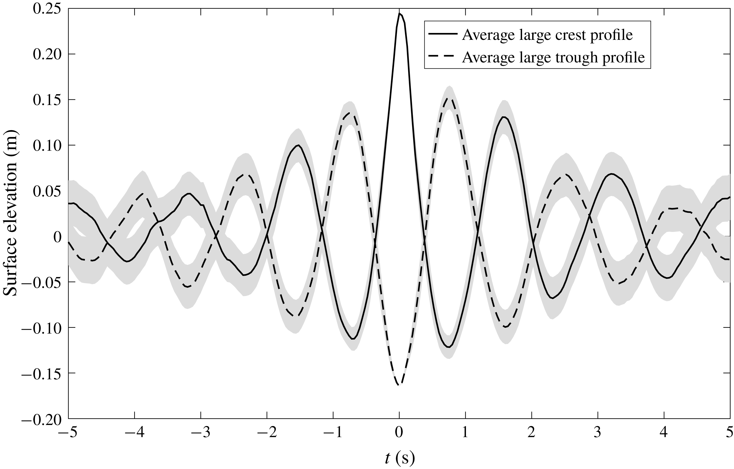
Figure 1. Average largest crest and trough profiles from the Lake George dataset with Lindgren variance shaded following the approach of Santo et al. (Reference Santo, Taylor, Eatock Taylor and Choo2013).
2 Data
In the paper, we examine extreme waves from two distinct datasets: Lake George and the North Sea. We present some background to these datasets in §§ 2.1 and 2.2 before considering the types of sea states present in each in § 2.3.
2.1 Description of the Lake George dataset
Surface elevation measurements taken from the Lake George field experiment site are a part of the integrated datasets obtained by Young et al. (Reference Young, Banner, Donelan, McCormick, Babanin, Melville and Veron2005). The measurement campaign lasted from September 1997 to May 1999. The geographical layout of Lake George is shown in figure 2, indicating a large lake with a fairly flat bed. Previous experiments at Lake George successfully determined the spectral evolution of wind-generated waves (Young & Verhagen Reference Young and Verhagen1996) and the directional spectrum with the implementation of wave arrays using the maximum likelihood method (MLM) (Young Reference Young1994; Young, Verhagen & Banner Reference Young, Verhagen and Banner1995). Based on prior experience, a project was established to investigate the physics behind the steep and narrow-banded waves at a new experimental site shown in figure 2. During this project, a spatial array consisting of eight capacitance probes was deployed to determine the surface elevation at a resolution of 25 Hz (Young et al.
Reference Young, Banner, Donelan, McCormick, Babanin, Melville and Veron2005). The detailed configuration is shown in figure 3: five probes were separated evenly in a 30 cm diameter circle and another three probes were placed in the middle. These probes measured high-quality wave records, with values of peak frequency
 $f_{p}$
ranging from 0.33 to 0.5 Hz and values of significant wave height
$f_{p}$
ranging from 0.33 to 0.5 Hz and values of significant wave height
 $H_{s}$
varying from 0.08 to 0.5 m.
$H_{s}$
varying from 0.08 to 0.5 m.
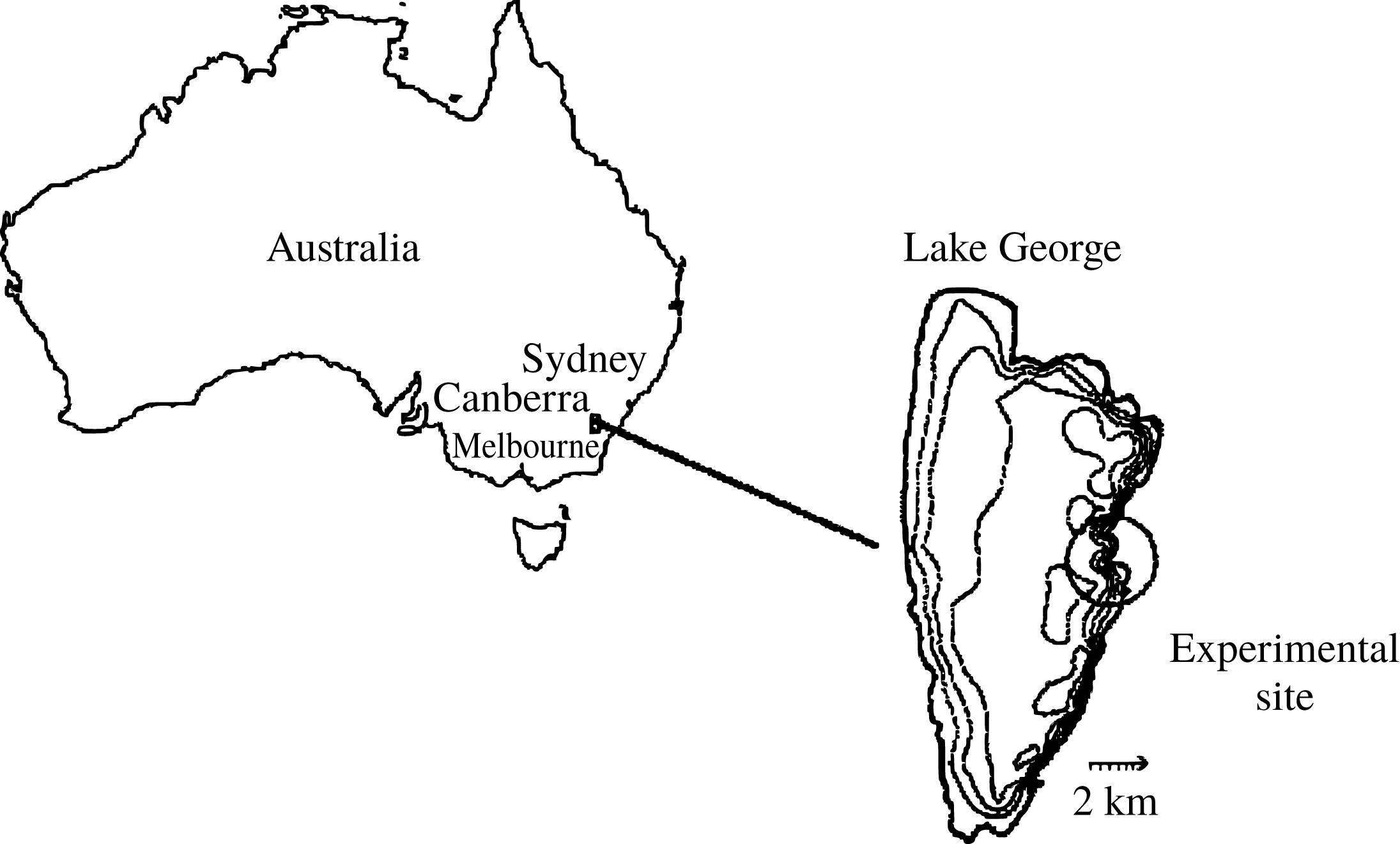
Figure 2. Location of the Lake George site (taken from Babanin, Young & Banner (Reference Babanin, Young and Banner2001)).

Figure 3. Configuration of the capacitance array.
As a part of the integrated dataset, the wave elevation records have been used for many purposes. Babanin et al. (Reference Babanin, Young and Banner2001) applied the data together with video records and acoustic signals to obtain the breaking probability at finite depth. They also used the spectral properties of wave elevation data as well as wind data to address the dependence of drag coefficient on wind speed, sea state and gustiness (Babanin & Makin Reference Babanin and Makin2008). In addition, Toffoli et al. (Reference Toffoli, Monbaliu, Onorato, Osborne, Babanin and Bitner-Gregersen2007) also analysed the statistical properties of wave crests to validate the numerical simulation of second-order wave theory.
During the measurement period, as part of natural hydrology cycles, the lake was drying out gradually, with the water depth dropping from 1.1 m in 1997 to 0.4 m in 1999. In this study, we use a pre-filtering process to exclude the time series with
 $H_{s}$
less than 0.1 m or the non-dimensional water depth
$H_{s}$
less than 0.1 m or the non-dimensional water depth
 $k_{p}d$
(where
$k_{p}d$
(where
 $k_{p}$
is the peak wavenumber and
$k_{p}$
is the peak wavenumber and
 $d$
is the water depth) less than 1.6. This confines the data to be more representative of developed wind-generated waves at deep and intermediate water depths. Additionally, a rigorous data quality control procedure is applied to each dataset to remove instrumental errors and to produce a reliable dataset following the approach of Christou & Ewans (Reference Christou and Ewans2014).
$d$
is the water depth) less than 1.6. This confines the data to be more representative of developed wind-generated waves at deep and intermediate water depths. Additionally, a rigorous data quality control procedure is applied to each dataset to remove instrumental errors and to produce a reliable dataset following the approach of Christou & Ewans (Reference Christou and Ewans2014).
2.2 Description of the North Sea dataset
The North Sea dataset contains a large amount of wave and wind data taken from several oil platforms in the North Sea (see figure 4 for detailed locations). The measurement period started on November 2013 and ran for four consecutive months. The collected data are then divided into 30 min time series, and over 43 000 wave records are analysed in the project. The large amount of wave records provide an insight into wave behaviour in the North Sea, with several storms observed.

Figure 4. North Sea data locations.
The data were measured by downward-looking SAAB radars installed at the side of the platforms. All the data were from fixed jacket structures and not from buoys. Measuring waves in the harsh maritime environment is very difficult. The accuracy of different measuring methods is not known definitively, but studies such as Forristall et al. (Reference Forristall, Barstow, Krogstad, Prevosto, Taylor and Tromans2004) suggest that radar measurements are not as accurate as a laser or a wave staff, but that the measurements from radars are still useful. Ewans, Jonathan & Feld (Reference Ewans, Jonathan and Feld2013) have looked in detail at the performances of wave radars, and their recent work (Ewans, Feld & Jonathan Reference Ewans, Feld and Jonathan2014) shows that the SAAB radars in the North Sea have no obvious bias.
Field measurement made by wave radars have been used by numerous authors, including Christou & Ewans’s (Reference Christou and Ewans2014) major study of rogue waves. Other examples of using radars for the analysis of extreme waves include Taylor & Williams (Reference Taylor and Williams2004) and Bell, Gray & Jones (Reference Bell, Gray and Jones2017), who examined the average properties of extreme waves. Whilst we think measurements made with wave radar are accurate enough for analysis, particularly where an average is taken over many records, some caution should be applied to any calculations drawn from wave radar data.
The measuring frequency is 2 Hz. Since there is no exact description of the rig for each platform, all the time series within the North Sea dataset are assumed to be free-field measurements, although wave–structure interactions can be significant for some platforms. Possible sources of error are considered further in the discussions.
After the initial inspection for missing entries, all the time series are filtered to remove any background noise over
 $4~\text{rad}~\text{s}^{-1}$
. The filtered time series are then processed using the same quality check approach as the one used for the Lake George dataset to obtain reliable wave records. The North Sea records have
$4~\text{rad}~\text{s}^{-1}$
. The filtered time series are then processed using the same quality check approach as the one used for the Lake George dataset to obtain reliable wave records. The North Sea records have
 $H_{s}$
varying from 0.38 m to 13.33 m and the zero-crossing frequency,
$H_{s}$
varying from 0.38 m to 13.33 m and the zero-crossing frequency,
 $f_{z}$
, between
$f_{z}$
, between
 $0.54~\text{rad}~\text{s}^{-1}$
and
$0.54~\text{rad}~\text{s}^{-1}$
and
 $1.95~\text{rad}~\text{s}^{-1}$
.
$1.95~\text{rad}~\text{s}^{-1}$
.
2.3 Comparison of two datasets
Owing to the location of the measurement and the instrumentation, there are several significant differences between the wave elevation records from the two datasets. The location of the Lake George dataset allows the deployment of high-quality elevation probes, which provides high-quality data with higher sampling frequency and less disturbance from the rig. Additionally, there is no swell or tidal variation for the Lake George dataset. However, the total amount of available records is significantly less than for the North Sea dataset, leading to more statistical variation in our analysis.
For comparison purposes, some basic parameters from both datasets are presented. In figure 5 the zero-crossing period
 $T_{z}$
is plotted against significant wave height
$T_{z}$
is plotted against significant wave height
 $H_{s}$
from both datasets. Additionally, lines of constant mean steepness of the sea state are also presented for comparison, as the steepness is a key measurement of nonlinearity. Steepness for deep water waves is given by
$H_{s}$
from both datasets. Additionally, lines of constant mean steepness of the sea state are also presented for comparison, as the steepness is a key measurement of nonlinearity. Steepness for deep water waves is given by
 $$\begin{eqnarray}\text{steepness}=\frac{2\unicode[STIX]{x03C0}}{g}\frac{H_{s}}{T_{z}^{2}},\end{eqnarray}$$
where
 $g$
is the gravitational acceleration. Although the wave height of the Lake George data is relatively small, these records are exceptionally steep.
$g$
is the gravitational acceleration. Although the wave height of the Lake George data is relatively small, these records are exceptionally steep.
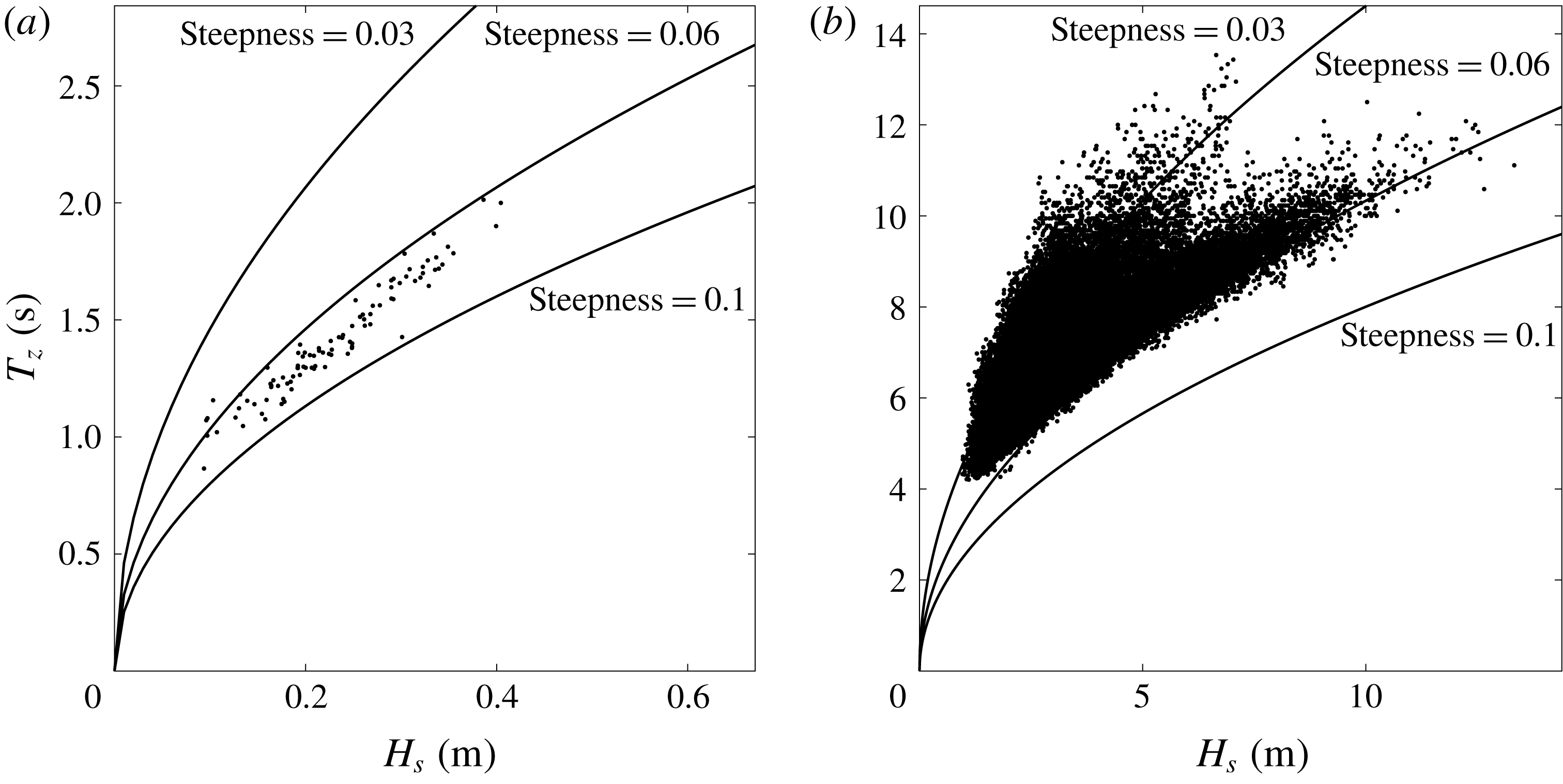
Figure 5. Scatterplot for
 $H_{s}$
and
$H_{s}$
and
 $T_{z}$
from (a) Lake George and (b) the North Sea.
$T_{z}$
from (a) Lake George and (b) the North Sea.
As well as steepness, another key parameter measuring the nonlinearity of wave recordings is the Benjamin–Feir index (BFI) proposed by Janssen (Reference Janssen2003). In this paper, the approach of Serio et al. (Reference Serio, Onorato, Osborne and Janssen2005) is adapted to compute the BFI from the time series:
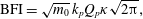 $$\begin{eqnarray}\text{BFI}=\sqrt{m_{0}}\,k_{p}Q_{p}\unicode[STIX]{x1D705}\sqrt{2\unicode[STIX]{x03C0}},\end{eqnarray}$$
where
 $m_{0}=H_{s}^{2}/16$
is the zeroth moment of the energy spectrum, and
$m_{0}=H_{s}^{2}/16$
is the zeroth moment of the energy spectrum, and
 $\unicode[STIX]{x1D705}$
is a depth correction factor, which is unity in deep water, and can be computed as
$\unicode[STIX]{x1D705}$
is a depth correction factor, which is unity in deep water, and can be computed as
 $$\begin{eqnarray}\unicode[STIX]{x1D705}=\unicode[STIX]{x1D707}\sqrt{\frac{|\unicode[STIX]{x1D70F}|}{\unicode[STIX]{x1D712}}},\end{eqnarray}$$
where
 $\unicode[STIX]{x1D707}$
,
$\unicode[STIX]{x1D707}$
,
 $\unicode[STIX]{x1D70F}$
and
$\unicode[STIX]{x1D70F}$
and
 $\unicode[STIX]{x1D712}$
are all dimensionless coefficients depending on relative water depth
$\unicode[STIX]{x1D712}$
are all dimensionless coefficients depending on relative water depth
 $k_{p}d$
. The general forms of
$k_{p}d$
. The general forms of
 $\unicode[STIX]{x1D707}$
,
$\unicode[STIX]{x1D707}$
,
 $\unicode[STIX]{x1D70F}$
and
$\unicode[STIX]{x1D70F}$
and
 $\unicode[STIX]{x1D712}$
are reported (see Mei (Reference Mei1989) for detailed derivation) as
$\unicode[STIX]{x1D712}$
are reported (see Mei (Reference Mei1989) for detailed derivation) as
 $$\begin{eqnarray}\displaystyle & \displaystyle \unicode[STIX]{x1D707}=1+2\frac{k_{p}d}{\sinh (2k_{p}d)}, & \displaystyle\end{eqnarray}$$
 $$\begin{eqnarray}\displaystyle & \displaystyle \unicode[STIX]{x1D70F}=-\unicode[STIX]{x1D707}^{2}+2+8(k_{p}d)^{2}\frac{\cosh (2k_{p}d)}{\sinh ^{2}(2k_{p}d)}, & \displaystyle\end{eqnarray}$$
 $$\begin{eqnarray}\displaystyle & \displaystyle \unicode[STIX]{x1D712}=\frac{\cosh (4k_{p}d)+8-2\tanh ^{2}(k_{p}d)}{8\sinh ^{4}(k_{p}d)}-\frac{(2\cosh ^{2}(k_{p}d)+0.5\unicode[STIX]{x1D707})^{2}}{\sinh ^{2}(2k_{p}d)\left[\displaystyle \frac{k_{p}d}{\tanh (k_{p}d)}-\left(\frac{\unicode[STIX]{x1D707}}{2}\right)^{2}\right]}. & \displaystyle\end{eqnarray}$$
Here
 $Q_{p}$
is the quality factor, introduced by Goda (Reference Goda2000);
$Q_{p}$
is the quality factor, introduced by Goda (Reference Goda2000);
 $Q_{p}$
is a dimensionless parameter that describes the spectral bandwidth. It has less sensitivity to the high-frequency tail of the spectrum (and cutoff frequency) than other bandwidth metrics (Prasada Rao Reference Prasada Rao1988; Serio et al.
Reference Serio, Onorato, Osborne and Janssen2005);
$Q_{p}$
is a dimensionless parameter that describes the spectral bandwidth. It has less sensitivity to the high-frequency tail of the spectrum (and cutoff frequency) than other bandwidth metrics (Prasada Rao Reference Prasada Rao1988; Serio et al.
Reference Serio, Onorato, Osborne and Janssen2005);
 $Q_{p}$
is given by
$Q_{p}$
is given by
 $$\begin{eqnarray}Q_{p}=\frac{2}{{m_{0}}^{2}}\int _{0}^{\infty }f\,S^{2}(f)\,\text{d}f,\end{eqnarray}$$
where
 $S(f)$
is the wave spectral density function.
$S(f)$
is the wave spectral density function.
Hence, the quality factor with depth correction and the steepness for each dataset are computed in figure 6 with constant lines of BFI. Although containing fewer records, the majority of the Lake George dataset have higher BFI value than the North Sea dataset. Although the BFI is not a perfect parameter for describing nonlinearity (it does not contain any information on directional spreading, which is known to be important), it is remarkable that several values are close to the critical
 $\text{BFI}=1$
line, yet no data exceed this with the depth correction factor.
$\text{BFI}=1$
line, yet no data exceed this with the depth correction factor.
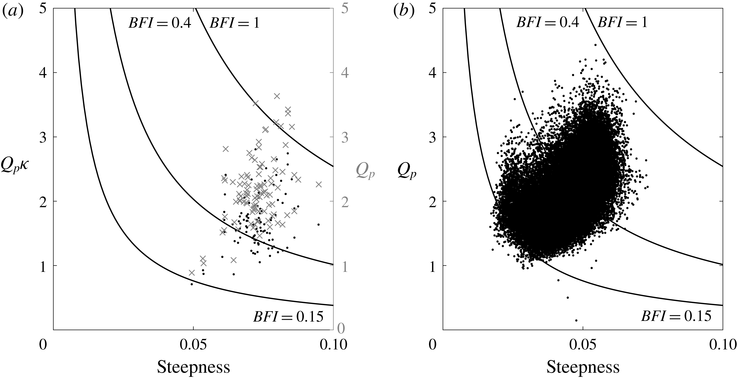
Figure 6. Scatterplot for steepness and quality factor from (a) Lake George (the secondary right-hand axis with ‘
 $\times$
’ markers shows the quality factor without depth correction) and (b) the North Sea (depth correction does not affect the quality factor in deep water).
$\times$
’ markers shows the quality factor without depth correction) and (b) the North Sea (depth correction does not affect the quality factor in deep water).
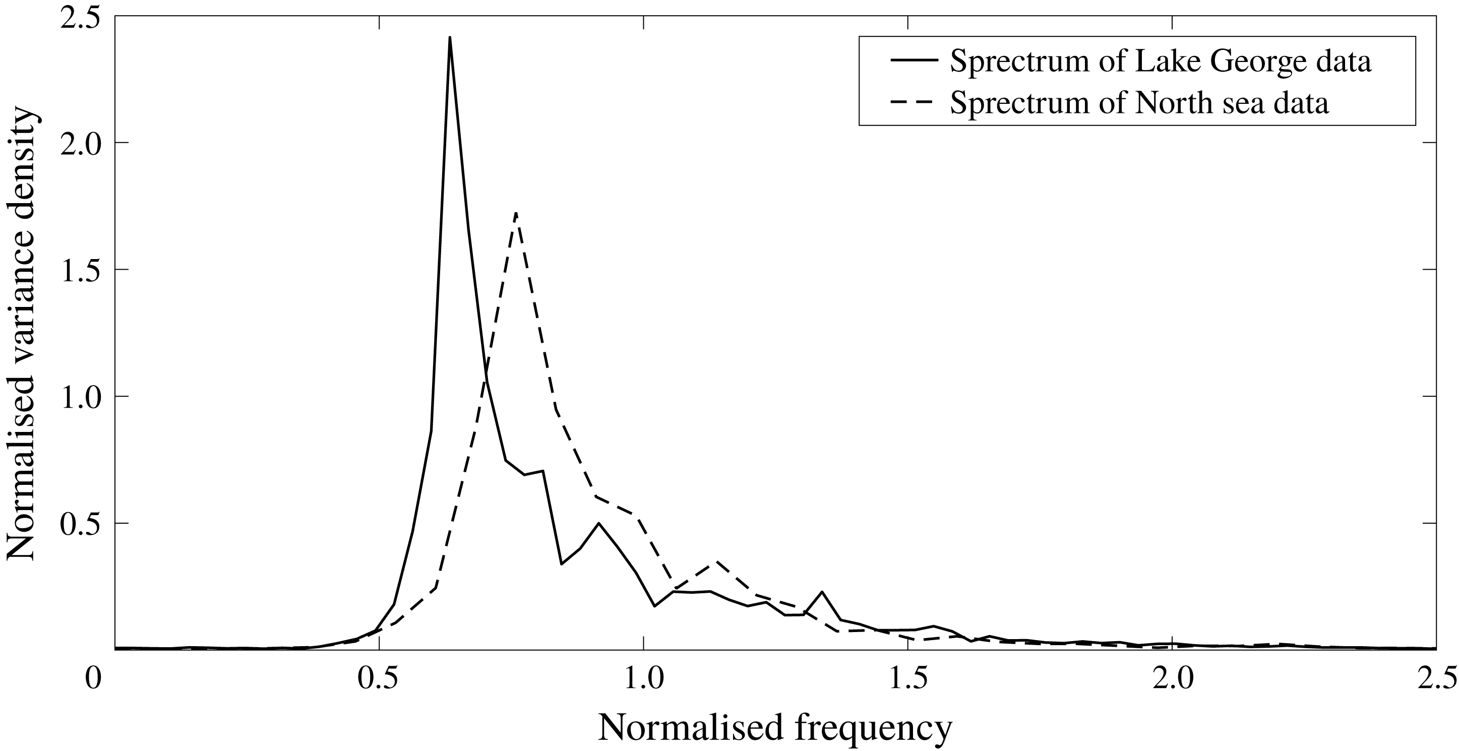
Figure 7. Comparison of typical Lake George spectrum with North Sea data normalised by the zeroth moment
 $m_{0}$
and zero-crossing frequency
$m_{0}$
and zero-crossing frequency
 $f_{z}$
of the individual wave record.
$f_{z}$
of the individual wave record.
2.4 Typical spectrum
The wave spectrum is the basic tool used to analyse a sea state. A sea state varies over time, so each time series has a different spectrum. Nonetheless, it is useful to present a typical omnidirectional spectrum for a wave record taken from the Lake George dataset and the North Sea dataset, respectively, which are shown in figure 7. A Tukey window is applied before the fast Fourier transform to prevent spectral leakage. The spectra are generated based on the average of 30 non-overlapping segments, which are then normalised by
 $m_{0}$
and
$m_{0}$
and
 $f_{z}$
of the wave record for comparison.
$f_{z}$
of the wave record for comparison.
One significant difference between the two spectra is that the Lake George dataset is more narrow-banded, which is probably due to the records in the North Sea dataset being well developed whereas there are quite a few relatively young waves in the Lake George dataset. This is consistent with figure 6, where the Lake George dataset tends to have a higher quality factor (over 5 % in the mean value) without the depth correction
 $\unicode[STIX]{x1D705}$
(i.e. low spectral bandwidth) on the secondary axis. However, the depth correction factor does not modify the quality factor in the North Sea dataset, as the water is rather deep at these oil platforms. Along with the steepness, spectral bandwidth and degree of directional spreading are key factors, which are expected to influence the nonlinear physics investigated by us in this paper (Adcock & Taylor Reference Adcock and Taylor2016).
$\unicode[STIX]{x1D705}$
(i.e. low spectral bandwidth) on the secondary axis. However, the depth correction factor does not modify the quality factor in the North Sea dataset, as the water is rather deep at these oil platforms. Along with the steepness, spectral bandwidth and degree of directional spreading are key factors, which are expected to influence the nonlinear physics investigated by us in this paper (Adcock & Taylor Reference Adcock and Taylor2016).
The directional spectrum for the Lake George dataset is also obtained using the MLM (Young Reference Young1994). The spreading parameters of these spectra indicate that the spreading angle is generally less than a broadly spread wind sea. However, we found our estimates of directional spread to be noisy and therefore these numbers are not reported in detail. Unfortunately, there was no directional spreading information available for the North Sea dataset, which consists of Eulerian point measurements from which it is challenging to estimate the exact directional spreading (Adcock & Taylor Reference Adcock and Taylor2009). Nevertheless, we would expect directional spreads to be mainly ‘following’ sea states with a small number of crossing seas. See for instance the North Sea data reported in McAllister, Venugopal & Borthwick (Reference McAllister, Venugopal and Borthwick2017).
3 Results
For the Lake George dataset, a total of 256 sets of data were collected in a fairly controlled environment (Young et al. Reference Young, Banner, Donelan, McCormick, Babanin, Melville and Veron2005), and 98 of them are within the scope of this paper after performing pre-filtering and data quality check. Each set of data contains eight 20 min time series, which were captured by eight capacitance probes (see figure 3) simultaneously. Owing to the probes in the array being quite close to each other compared to the typical wavelength (see figure 3), the measurements from one probe with the highest consistency (i.e. no significant departure in wave statistics from the measurements obtained by the probes nearby) are presented here. Meanwhile, the North Sea dataset has 43 000 usable 30 min time series. In the following subsections, the data will be processed to investigate horizontal asymmetry using three different parameters, as each gives a slightly different insight into the problem: the elevation difference between three successive large crests, the height difference between either side of the envelope, and the change in envelope width due to the sea state variation.
3.1 Analysis of raw time series
We start by analysing the relatively raw (although quality controlled) time series for both datasets. Our aim here is to demonstrate that the key phenomenon observed in the study does not result from some of the post-processing techniques used to obtain greater insight into the data in subsequent sections.
To assess the horizontal asymmetry properties of the raw wave records from the Lake George and the North Sea dataset, a robust data processing method is applied to find the difference between the preceding crest height and the following crest height of the largest waves. We analyse the largest five crests/waves in each time series – an example is shown in figure 8. This process is also restricted by a rule that the largest waves must be separated by a minimum distance of two zero-crossing periods to prevent selecting multiple waves from the same wave group. Afterwards, a parameter
 $\unicode[STIX]{x1D6FC}$
is defined to measure the relative ratio of adjacent crests to the largest one, which is similar to the measurement of unexpectedness established by Gemmrich & Thomson (Reference Gemmrich and Thomson2017). Here,
$\unicode[STIX]{x1D6FC}$
is defined to measure the relative ratio of adjacent crests to the largest one, which is similar to the measurement of unexpectedness established by Gemmrich & Thomson (Reference Gemmrich and Thomson2017). Here,
 $\unicode[STIX]{x1D6FC}$
is measured by the preceding wave crest
$\unicode[STIX]{x1D6FC}$
is measured by the preceding wave crest
 $\unicode[STIX]{x1D702}_{p}$
or following wave crest
$\unicode[STIX]{x1D702}_{p}$
or following wave crest
 $\unicode[STIX]{x1D702}_{f}$
in relation to the largest crest
$\unicode[STIX]{x1D702}_{f}$
in relation to the largest crest
 $\unicode[STIX]{x1D702}_{max}$
in this wave group (figure 8):
$\unicode[STIX]{x1D702}_{max}$
in this wave group (figure 8):
 $$\begin{eqnarray}\unicode[STIX]{x1D6FC}_{1}=\frac{\unicode[STIX]{x1D702}_{p}}{\unicode[STIX]{x1D702}_{max}},\quad \unicode[STIX]{x1D6FC}_{2}=\frac{\unicode[STIX]{x1D702}_{f}}{\unicode[STIX]{x1D702}_{max}}.\end{eqnarray}$$
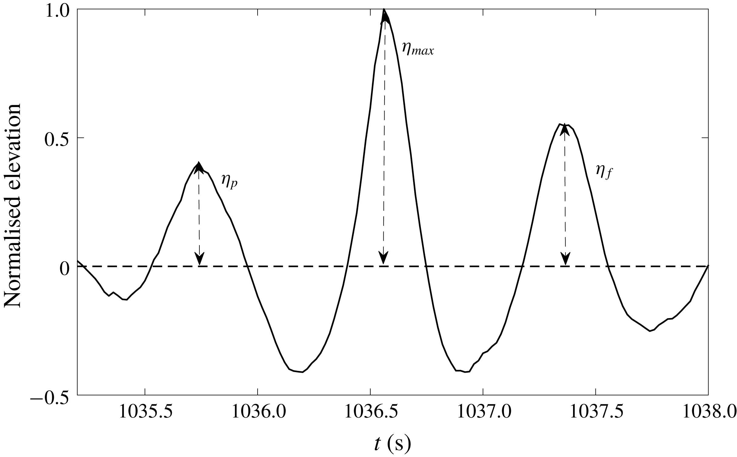
Figure 8. Illustration of the relative height of preceding and following crests.
After mass processing each wave record from the two pre-filtered datasets, the mean values of
 $\unicode[STIX]{x1D6FC}_{1}$
and
$\unicode[STIX]{x1D6FC}_{1}$
and
 $\unicode[STIX]{x1D6FC}_{2}$
are calculated by averaging the top five largest crests. The mean values are then categorised into different bins based on two sea state parameters: mean steepness, and the ratio between maximum crests
$\unicode[STIX]{x1D6FC}_{2}$
are calculated by averaging the top five largest crests. The mean values are then categorised into different bins based on two sea state parameters: mean steepness, and the ratio between maximum crests
 $\unicode[STIX]{x1D702}_{max}$
in each time series and significant wave height
$\unicode[STIX]{x1D702}_{max}$
in each time series and significant wave height
 $(H_{s})$
. The mean steepness is a key measurement for nonlinearity, whereas the ratio
$(H_{s})$
. The mean steepness is a key measurement for nonlinearity, whereas the ratio
 $\unicode[STIX]{x1D702}_{max}/H_{s}$
shows how big the largest waves are relative to the underlying sea state. The average mean values of
$\unicode[STIX]{x1D702}_{max}/H_{s}$
shows how big the largest waves are relative to the underlying sea state. The average mean values of
 $\unicode[STIX]{x1D6FC}_{1}$
and
$\unicode[STIX]{x1D6FC}_{1}$
and
 $\unicode[STIX]{x1D6FC}_{2}$
from each bin are presented in figure 9. To get a measure of the statistical validity, we use bootstrapping to give a 90 % confidence interval on the mean value of each bin (Efron & Tibshirani Reference Efron and Tibshirani1994).
$\unicode[STIX]{x1D6FC}_{2}$
from each bin are presented in figure 9. To get a measure of the statistical validity, we use bootstrapping to give a 90 % confidence interval on the mean value of each bin (Efron & Tibshirani Reference Efron and Tibshirani1994).
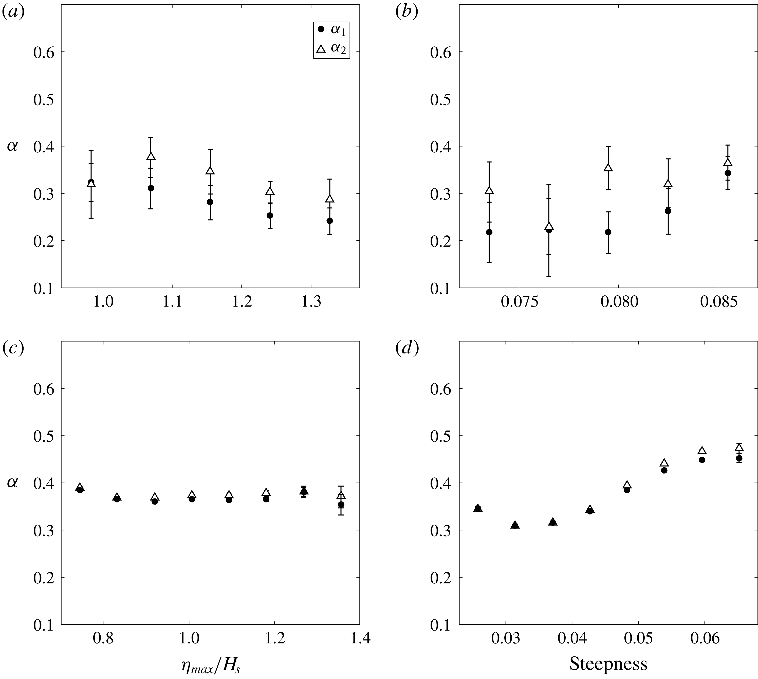
Figure 9. Relative height of preceding and following crests from (a,b) Lake George data and (c,d) North Sea data, for different (a,c) normalised maximum elevation and (b,d) mean steepness.
In figure 9(a,c), the
 $\unicode[STIX]{x1D6FC}$
values are divided into small bins based on the
$\unicode[STIX]{x1D6FC}$
values are divided into small bins based on the
 $\unicode[STIX]{x1D702}_{max}/H_{s}$
ratio, which shows a clear separation between
$\unicode[STIX]{x1D702}_{max}/H_{s}$
ratio, which shows a clear separation between
 $\unicode[STIX]{x1D6FC}_{1}$
and
$\unicode[STIX]{x1D6FC}_{1}$
and
 $\unicode[STIX]{x1D6FC}_{2}$
for the Lake George dataset. This indicates that the largest crests in the Lake George dataset tend to have a relatively smaller crest at the front and a larger crest at the back, which is consistent with the numerical simulation proposed by Lo & Mei (Reference Lo and Mei1985) in a unidirectional numerical wave tank and Adcock et al. (Reference Adcock, Taylor and Draper2015) for directional spread waves. However, for the open ocean data (figure 9
c),
$\unicode[STIX]{x1D6FC}_{2}$
for the Lake George dataset. This indicates that the largest crests in the Lake George dataset tend to have a relatively smaller crest at the front and a larger crest at the back, which is consistent with the numerical simulation proposed by Lo & Mei (Reference Lo and Mei1985) in a unidirectional numerical wave tank and Adcock et al. (Reference Adcock, Taylor and Draper2015) for directional spread waves. However, for the open ocean data (figure 9
c),
 $\unicode[STIX]{x1D6FC}_{1}$
and
$\unicode[STIX]{x1D6FC}_{1}$
and
 $\unicode[STIX]{x1D6FC}_{2}$
seem to be coincident with each other for a relatively small
$\unicode[STIX]{x1D6FC}_{2}$
seem to be coincident with each other for a relatively small
 $\unicode[STIX]{x1D702}_{max}/H_{s}$
ratio, but the difference becomes more evident for the wave records with the presence of rogue waves (defined as
$\unicode[STIX]{x1D702}_{max}/H_{s}$
ratio, but the difference becomes more evident for the wave records with the presence of rogue waves (defined as
 $\unicode[STIX]{x1D702}/H_{s}\geqslant 1.25$
).
$\unicode[STIX]{x1D702}/H_{s}\geqslant 1.25$
).
Additionally, both
 $\unicode[STIX]{x1D6FC}_{1}$
and
$\unicode[STIX]{x1D6FC}_{1}$
and
 $\unicode[STIX]{x1D6FC}_{2}$
seem to have a decreasing trend for the Lake George dataset, when the records contain larger waves. This phenomenon could be attributed to a nonlinear contraction to the wave group but could also be accounted for in different ways. For instance, bound harmonics would increase the size of the largest wave relative to the wave on either side. Based on the same reasons, it is not surprising to find that there is no clear overall trend for the North Sea dataset.
$\unicode[STIX]{x1D6FC}_{2}$
seem to have a decreasing trend for the Lake George dataset, when the records contain larger waves. This phenomenon could be attributed to a nonlinear contraction to the wave group but could also be accounted for in different ways. For instance, bound harmonics would increase the size of the largest wave relative to the wave on either side. Based on the same reasons, it is not surprising to find that there is no clear overall trend for the North Sea dataset.
In figure 9(b,d), the
 $\unicode[STIX]{x1D6FC}$
values are categorised by the steepness of the underlying sea state, which also shows a clear difference between the preceding crest height and the following crest height for the Lake George dataset. Although the separation shown in figure 9(d) for the North Sea dataset is not as significant as the previous one, this phenomenon can still be observed in the open ocean, especially for time series with a higher steepness value, which further confirms that there is some horizontal asymmetry in both datasets. However, a more detailed analysis is required to understand the trends involved.
$\unicode[STIX]{x1D6FC}$
values are categorised by the steepness of the underlying sea state, which also shows a clear difference between the preceding crest height and the following crest height for the Lake George dataset. Although the separation shown in figure 9(d) for the North Sea dataset is not as significant as the previous one, this phenomenon can still be observed in the open ocean, especially for time series with a higher steepness value, which further confirms that there is some horizontal asymmetry in both datasets. However, a more detailed analysis is required to understand the trends involved.
3.2 Analysis of envelope
To further analyse the horizontal asymmetry presented in § 3.1, a more delicate investigation into the envelope shape is conducted to demonstrate the horizontal asymmetry properties of the time series. The envelope
 $|U|$
is evaluated from the phase-resolved linearised free surface elevation to avoid the influence of bound harmonics (see appendix A for details) using
$|U|$
is evaluated from the phase-resolved linearised free surface elevation to avoid the influence of bound harmonics (see appendix A for details) using
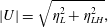 $$\begin{eqnarray}|U|=\sqrt{\unicode[STIX]{x1D702}_{L}^{2}+\unicode[STIX]{x1D702}_{LH}^{2}},\end{eqnarray}$$
where
 $\unicode[STIX]{x1D702}_{LH}$
is the Hilbert transform of the linearised elevation record.
$\unicode[STIX]{x1D702}_{LH}$
is the Hilbert transform of the linearised elevation record.
To examine the asymmetrical properties of the envelope, a parameter
 $\unicode[STIX]{x1D6FD}$
, which is similar to the
$\unicode[STIX]{x1D6FD}$
, which is similar to the
 $\unicode[STIX]{x1D701}$
introduced by Adcock et al. (Reference Adcock, Taylor and Draper2015), is defined (see figure 10 for details) as the ratio between the envelope height (
$\unicode[STIX]{x1D701}$
introduced by Adcock et al. (Reference Adcock, Taylor and Draper2015), is defined (see figure 10 for details) as the ratio between the envelope height (
 $|U_{p}|$
and
$|U_{p}|$
and
 $|U_{f}|$
respectively) at half zero-crossing period
$|U_{f}|$
respectively) at half zero-crossing period
 $T_{z}$
before and after the maximum envelope height
$T_{z}$
before and after the maximum envelope height
 $|U_{max}|$
:
$|U_{max}|$
:
 $$\begin{eqnarray}\unicode[STIX]{x1D6FD}_{1}=\frac{|U_{p}|}{|U_{max}|},\quad \unicode[STIX]{x1D6FD}_{2}=\frac{|U_{f}|}{|U_{max}|}.\end{eqnarray}$$
For a linear random time series, the value of
 $\unicode[STIX]{x1D6FD}$
should be dependent on the spectral width. Indeed, in the linear model, the expected shape of an extreme event with unit amplitude is given by unit NewWave (Lindgren Reference Lindgren1970; Boccotti Reference Boccotti1983; Tromans et al.
Reference Tromans, Anatruk and Hagemeijer1991):
$\unicode[STIX]{x1D6FD}$
should be dependent on the spectral width. Indeed, in the linear model, the expected shape of an extreme event with unit amplitude is given by unit NewWave (Lindgren Reference Lindgren1970; Boccotti Reference Boccotti1983; Tromans et al.
Reference Tromans, Anatruk and Hagemeijer1991):
 $$\begin{eqnarray}\unicode[STIX]{x1D702}(t)=\frac{1}{m_{0}}\int _{0}^{\infty }S(f)\cos (2\unicode[STIX]{x03C0}ft)\,\text{d}f.\end{eqnarray}$$
To ensure that any observed trend is not due to the correlations between steepness and bandwidth, we have also analysed the shape of NewWave groups derived from the underlying spectra of the entire linearised background sea state. Figures 11(a) and 11(b) shows the variation of
 $\unicode[STIX]{x1D6FD}$
values for different
$\unicode[STIX]{x1D6FD}$
values for different
 $\unicode[STIX]{x1D702}_{max}/H_{s}$
ratios, in terms of linearised real time series and the corresponding NewWave profile. As for the real data, which are described in figure 11(a), the relative envelope height before the envelope maximum (
$\unicode[STIX]{x1D702}_{max}/H_{s}$
ratios, in terms of linearised real time series and the corresponding NewWave profile. As for the real data, which are described in figure 11(a), the relative envelope height before the envelope maximum (
 $\unicode[STIX]{x1D6FD}_{1}$
) is significantly less than that after the peak (
$\unicode[STIX]{x1D6FD}_{1}$
) is significantly less than that after the peak (
 $\unicode[STIX]{x1D6FD}_{2}$
). Moreover, the difference between
$\unicode[STIX]{x1D6FD}_{2}$
). Moreover, the difference between
 $\unicode[STIX]{x1D6FD}_{1}$
and
$\unicode[STIX]{x1D6FD}_{1}$
and
 $\unicode[STIX]{x1D6FD}_{2}$
seems to be more significant when an extreme wave occurs within the wave record, which is captured by a higher
$\unicode[STIX]{x1D6FD}_{2}$
seems to be more significant when an extreme wave occurs within the wave record, which is captured by a higher
 $\unicode[STIX]{x1D702}_{max}/H_{s}$
ratio. This will also lead to a decrease in both
$\unicode[STIX]{x1D702}_{max}/H_{s}$
ratio. This will also lead to a decrease in both
 $\unicode[STIX]{x1D6FD}_{1}$
and
$\unicode[STIX]{x1D6FD}_{1}$
and
 $\unicode[STIX]{x1D6FD}_{2}$
, which we suggest is caused by the nonlinear contraction of the wave group, as predicted by theory (Adcock et al.
Reference Adcock, Gibbs and Taylor2012). However, these three main trends for real linearised time series are not found in NewWave (see figure 11
b). The distinct difference between the real time series and the NewWave indicates that the apparent contraction of wave group is not a linear effect but due to some nonlinear changes during the extreme events.
$\unicode[STIX]{x1D6FD}_{2}$
, which we suggest is caused by the nonlinear contraction of the wave group, as predicted by theory (Adcock et al.
Reference Adcock, Gibbs and Taylor2012). However, these three main trends for real linearised time series are not found in NewWave (see figure 11
b). The distinct difference between the real time series and the NewWave indicates that the apparent contraction of wave group is not a linear effect but due to some nonlinear changes during the extreme events.
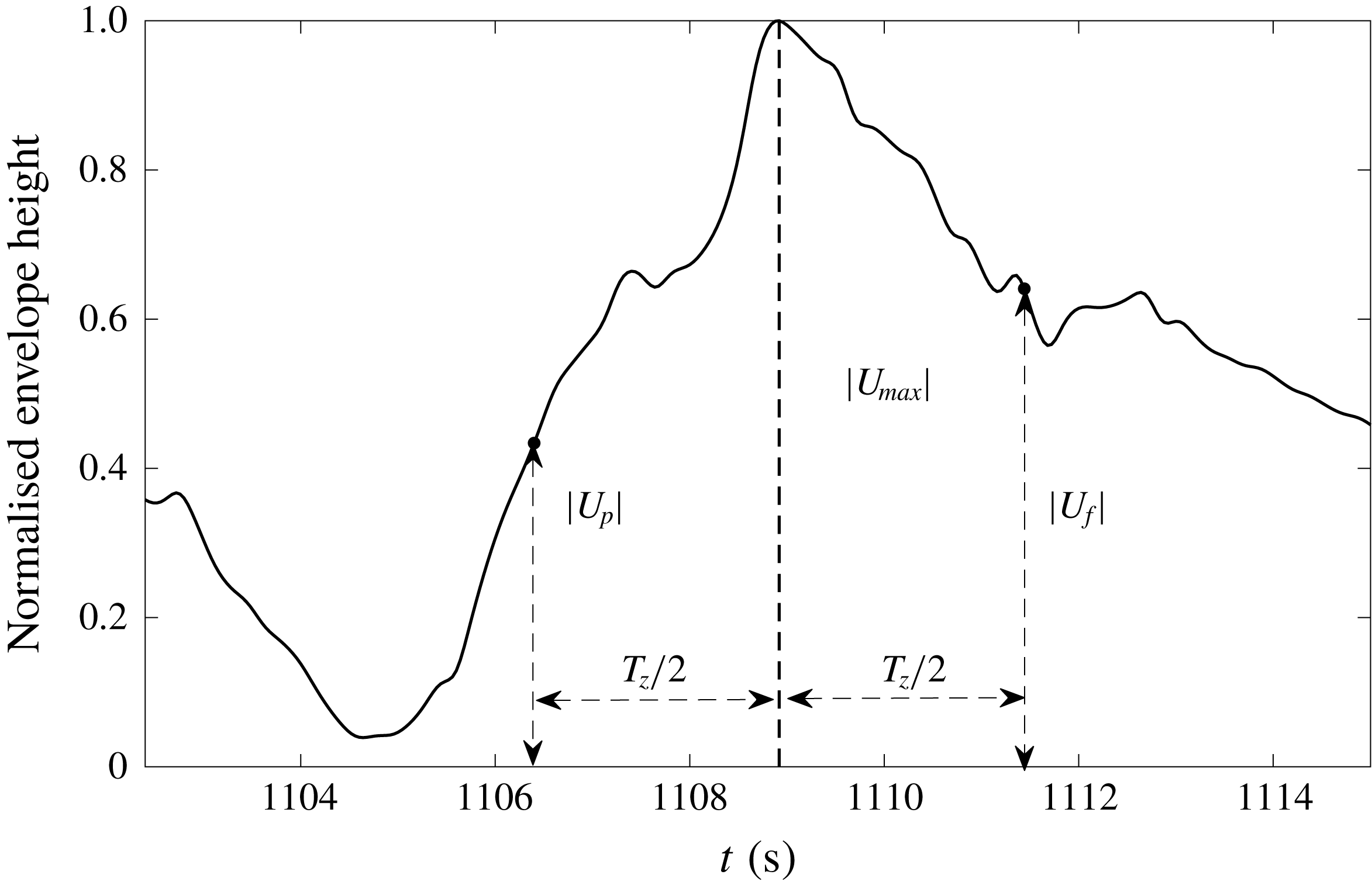
Figure 10. Illustration of the relative envelope height at
 $T_{z}/2$
away from the envelope maximum.
$T_{z}/2$
away from the envelope maximum.
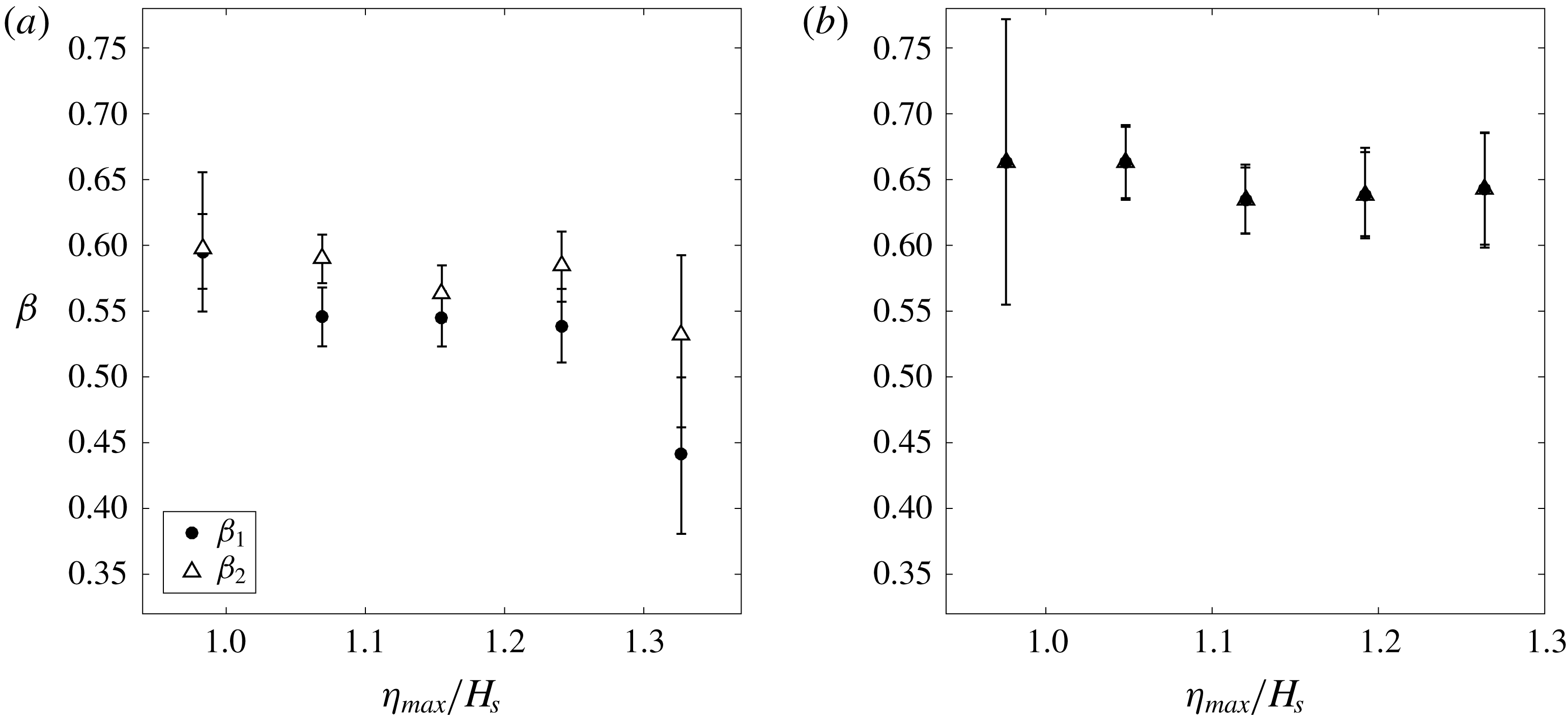
Figure 11. Envelope height half-period away from the peak at different normalised maximum elevations from the Lake George dataset for (a) linearised data and (b) NewWave.
However, the overall tendency of the
 $\unicode[STIX]{x1D6FD}_{1}$
and
$\unicode[STIX]{x1D6FD}_{1}$
and
 $\unicode[STIX]{x1D6FD}_{2}$
values for the North Sea dataset is not obvious, as the spectral bandwidth varies significantly with the change in both the
$\unicode[STIX]{x1D6FD}_{2}$
values for the North Sea dataset is not obvious, as the spectral bandwidth varies significantly with the change in both the
 $\unicode[STIX]{x1D702}_{max}/H_{s}$
ratio and the steepness. Hence, a new parameter
$\unicode[STIX]{x1D702}_{max}/H_{s}$
ratio and the steepness. Hence, a new parameter
 $B$
, which is defined as the ratio between
$B$
, which is defined as the ratio between
 $\unicode[STIX]{x1D6FD}_{measured}$
and
$\unicode[STIX]{x1D6FD}_{measured}$
and
 $\unicode[STIX]{x1D6FD}_{NewWave}$
, is established to describe the relative percentage of NewWave envelope taken by the envelope of measured data:
$\unicode[STIX]{x1D6FD}_{NewWave}$
, is established to describe the relative percentage of NewWave envelope taken by the envelope of measured data:
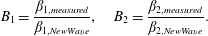 $$\begin{eqnarray}B_{1}=\frac{\unicode[STIX]{x1D6FD}_{1,measured}}{\unicode[STIX]{x1D6FD}_{1,NewWave}},\quad B_{2}=\frac{\unicode[STIX]{x1D6FD}_{2,measured}}{\unicode[STIX]{x1D6FD}_{2,NewWave}}.\end{eqnarray}$$
Although this parameter is perfect for describing the difference between the measured envelope and NewWave envelope, during data processing, the division also introduces some statistical uncertainty, which results in this parameter being unsuitable for a relatively small sized dataset i.e. the Lake George dataset.
In contrast, the confidence interval of North Sea results (over 43 000 usable time series) is still acceptable, which is shown in figure 12. In figure 12(a), the relationship between relative envelope ratio
 $B$
and the
$B$
and the
 $\unicode[STIX]{x1D702}_{max}/H_{s}$
ratio is established. Similar to the Lake George dataset, compared with the NewWave envelope, the measured relative envelope height at a half-period before the maximum (
$\unicode[STIX]{x1D702}_{max}/H_{s}$
ratio is established. Similar to the Lake George dataset, compared with the NewWave envelope, the measured relative envelope height at a half-period before the maximum (
 $B_{1}$
) is smaller than that after the maximum (
$B_{1}$
) is smaller than that after the maximum (
 $B_{2}$
), which indicates that there may be some horizontal asymmetry even in the open ocean. Moreover, the overall decreasing trend is also found in the North Sea dataset, which is believed to be caused by the nonlinear group contraction in mean wave direction. We note that, compared to the Lake George dataset, which is exceptionally steep, the horizontal asymmetry observed in the North Sea dataset is relatively small for most records.
$B_{2}$
), which indicates that there may be some horizontal asymmetry even in the open ocean. Moreover, the overall decreasing trend is also found in the North Sea dataset, which is believed to be caused by the nonlinear group contraction in mean wave direction. We note that, compared to the Lake George dataset, which is exceptionally steep, the horizontal asymmetry observed in the North Sea dataset is relatively small for most records.
In figure 12(b), relative envelope ratio
 $B$
is categorised based on the mean steepness, which presents two almost identical trends in figure 12(a):
$B$
is categorised based on the mean steepness, which presents two almost identical trends in figure 12(a):
 $B_{1}$
and
$B_{1}$
and
 $B_{2}$
are well separated especially for sea states with higher steepness value, and both
$B_{2}$
are well separated especially for sea states with higher steepness value, and both
 $B_{1}$
and
$B_{1}$
and
 $B_{2}$
decrease for steeper sea states. This indicates that the envelope tends to have a steeper front and a relatively flat tail, and the wave envelope tends to contract for steeper sea states. This further confirms that the nonlinear physics can also alter the shape of the envelope in the ocean. However, for relatively low steepness, both ratios
$B_{2}$
decrease for steeper sea states. This indicates that the envelope tends to have a steeper front and a relatively flat tail, and the wave envelope tends to contract for steeper sea states. This further confirms that the nonlinear physics can also alter the shape of the envelope in the ocean. However, for relatively low steepness, both ratios
 $B_{1}$
and
$B_{1}$
and
 $B_{2}$
are quite close to 1, which suggests that the NewWave is a good approximation for most extreme events in the open ocean.
$B_{2}$
are quite close to 1, which suggests that the NewWave is a good approximation for most extreme events in the open ocean.
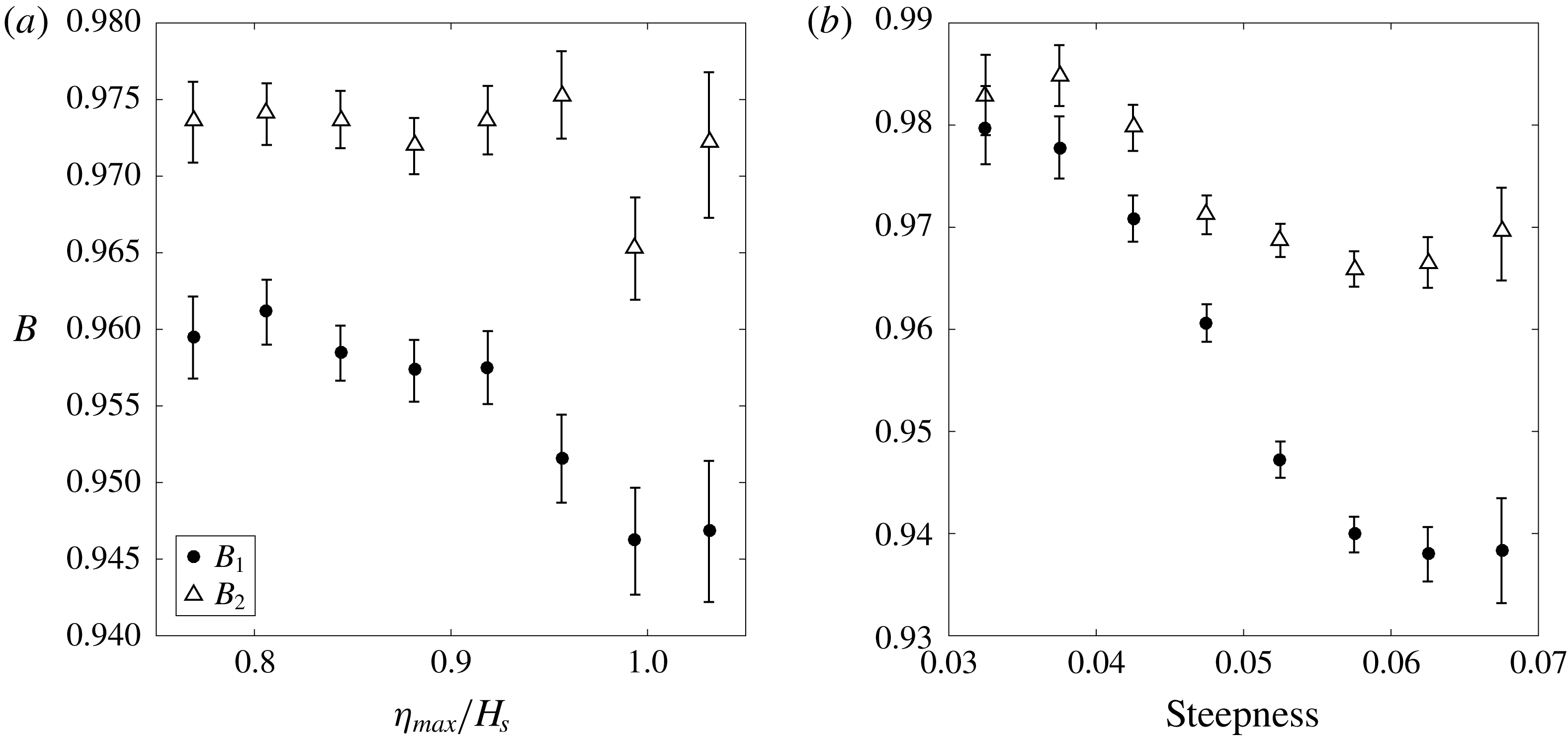
Figure 12. NewWave-based relative envelope height half-period away from the peak from the North Sea dataset for different (a) normalised maximum elevation and (b) mean steepness.
As an alternative approach to studying the shape of the wave package, a parameter
 $\unicode[STIX]{x1D70E}$
is established to measure the envelope width, which is similar to the group bandwidth presented by Adcock et al. (Reference Adcock, Taylor and Draper2015). The parameter is defined as the envelope width (
$\unicode[STIX]{x1D70E}$
is established to measure the envelope width, which is similar to the group bandwidth presented by Adcock et al. (Reference Adcock, Taylor and Draper2015). The parameter is defined as the envelope width (
 $\unicode[STIX]{x1D70E}_{1}$
and
$\unicode[STIX]{x1D70E}_{1}$
and
 $\unicode[STIX]{x1D70E}_{2}$
, respectively) on both sides between the envelope peak and the point where the envelope height is 80 % of the maximum of the envelope. Additionally, the total envelope width
$\unicode[STIX]{x1D70E}_{2}$
, respectively) on both sides between the envelope peak and the point where the envelope height is 80 % of the maximum of the envelope. Additionally, the total envelope width
 $\unicode[STIX]{x1D70E}_{total}$
is also presented for a better description of envelope width (see figure 13 for a detailed illustration).
$\unicode[STIX]{x1D70E}_{total}$
is also presented for a better description of envelope width (see figure 13 for a detailed illustration).
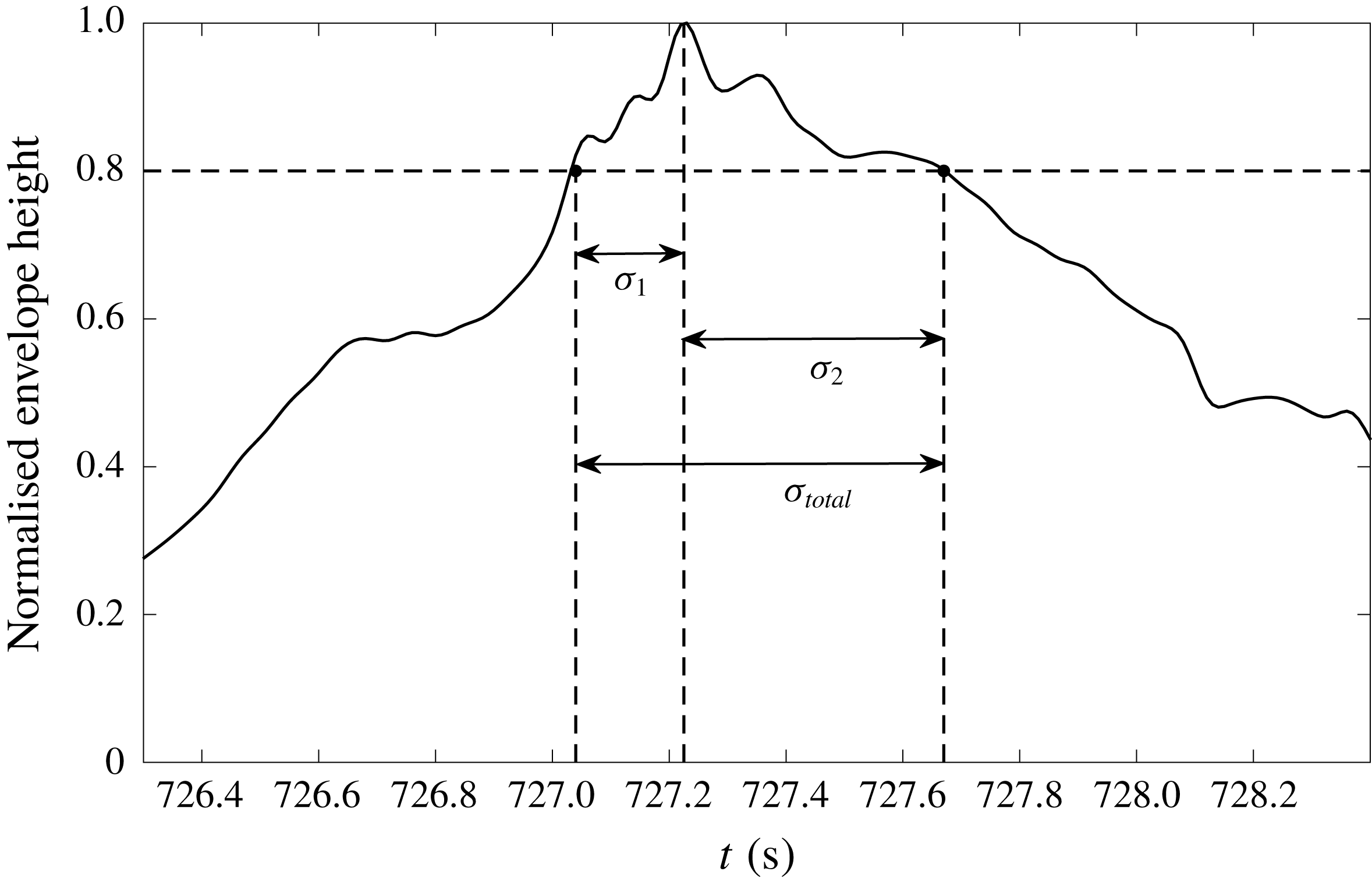
Figure 13. Illustration of the envelope width at
 $80\,\%$
of maximum peak height of the envelope.
$80\,\%$
of maximum peak height of the envelope.
The correlation between
 $\unicode[STIX]{x1D70E}$
and steepness for the Lake George dataset is plotted in figure 14 for both linearised real time series and NewWave derived from the spectrum. It is obvious that the envelope width before the envelope peak is less than that after the maximum for relatively steep wave records, which indicates stronger envelope horizontal asymmetry for steeper sea states. Additionally, with the increase in steepness of the sea state, the envelope becomes much narrower around the crest, which is consistent with the previous numerical simulation by Adcock et al. (Reference Adcock, Taylor and Draper2016) as well as some experiments (Shemer et al.
Reference Shemer, Kit, Jiao and Eitan1998), albeit in unidirectional waves. Additionally, the same check on NewWave is conducted to ensure that this phenomenon is not caused by the background spectrum. The envelope width of NewWave is much broader than measured data, which is also consistent with nonlinear physics causing a contraction of the wave group.
$\unicode[STIX]{x1D70E}$
and steepness for the Lake George dataset is plotted in figure 14 for both linearised real time series and NewWave derived from the spectrum. It is obvious that the envelope width before the envelope peak is less than that after the maximum for relatively steep wave records, which indicates stronger envelope horizontal asymmetry for steeper sea states. Additionally, with the increase in steepness of the sea state, the envelope becomes much narrower around the crest, which is consistent with the previous numerical simulation by Adcock et al. (Reference Adcock, Taylor and Draper2016) as well as some experiments (Shemer et al.
Reference Shemer, Kit, Jiao and Eitan1998), albeit in unidirectional waves. Additionally, the same check on NewWave is conducted to ensure that this phenomenon is not caused by the background spectrum. The envelope width of NewWave is much broader than measured data, which is also consistent with nonlinear physics causing a contraction of the wave group.
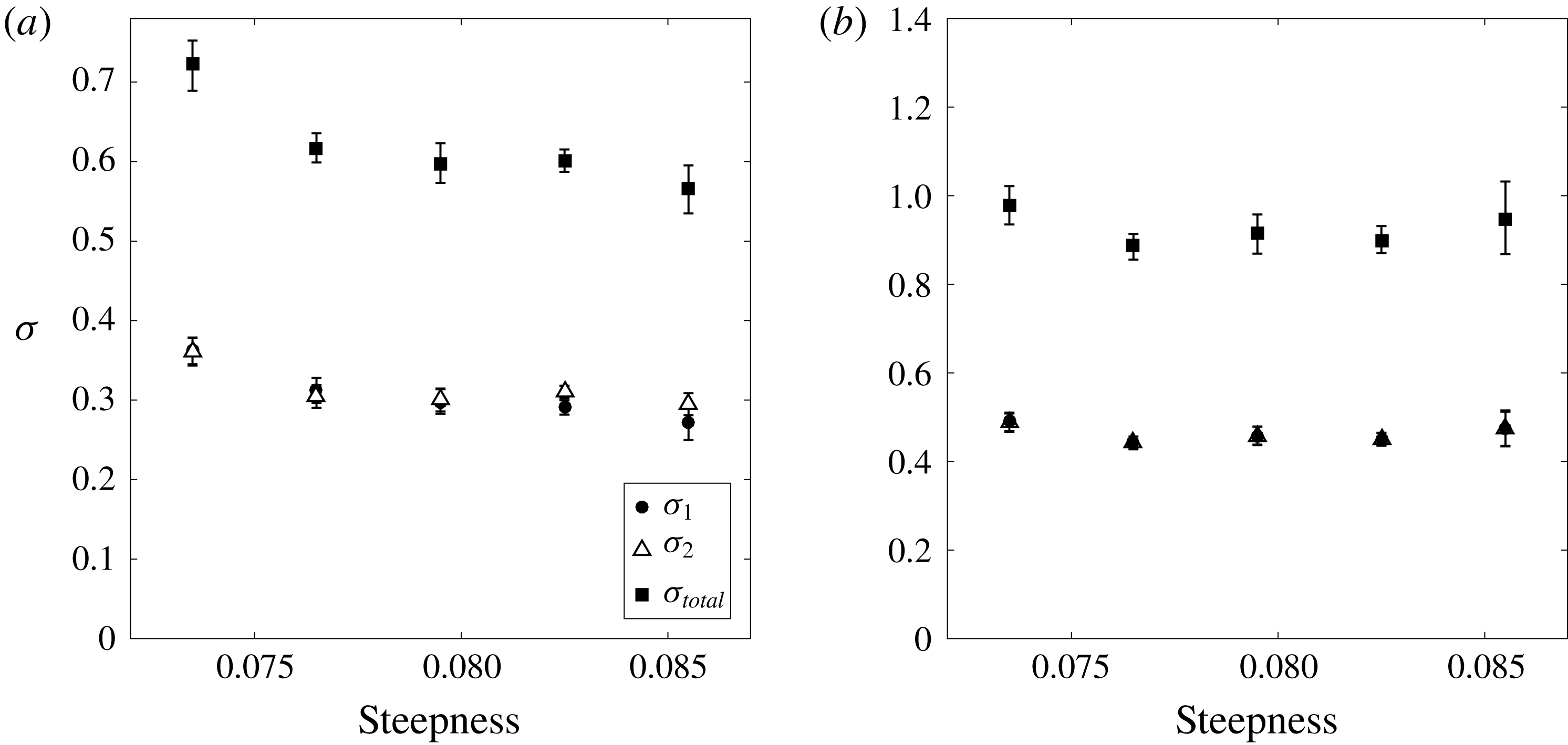
Figure 14. Envelope width at
 $80\,\%$
of maximum peak height from Lake George dataset at different steepness for (a) linearised data and (b) NewWave.
$80\,\%$
of maximum peak height from Lake George dataset at different steepness for (a) linearised data and (b) NewWave.
Figure 15 presents the results from analysing the envelope width from the North Sea dataset with the same data processing method. Owing to the fact that the envelope width in the linear model is highly dependent on the spectral bandwidth, the width of a NewWave group, which accounts for the variation in bandwidth, is used for normalisation. Therefore, a new parameter
 $\unicode[STIX]{x1D709}$
defined as the ratio of measured envelope width
$\unicode[STIX]{x1D709}$
defined as the ratio of measured envelope width
 $\unicode[STIX]{x1D70E}_{measured}$
to the
$\unicode[STIX]{x1D70E}_{measured}$
to the
 $\unicode[STIX]{x1D70E}_{NewWave}$
is computed as below:
$\unicode[STIX]{x1D70E}_{NewWave}$
is computed as below:
 $$\begin{eqnarray}\unicode[STIX]{x1D709}_{1}=\frac{\unicode[STIX]{x1D70E}_{1,measured}}{\unicode[STIX]{x1D70E}_{1,NewWave}},\quad \unicode[STIX]{x1D709}_{2}=\frac{\unicode[STIX]{x1D70E}_{2,measured}}{\unicode[STIX]{x1D70E}_{2,NewWave}}.\end{eqnarray}$$
The variation of this parameter in terms of the
 $\unicode[STIX]{x1D702}_{max}/H_{s}$
ratio and steepness is also presented in figures 15(a) and 15(b), respectively. Overall the result is very similar to figure 12, which indicates that there is a subtle but clear separation between
$\unicode[STIX]{x1D702}_{max}/H_{s}$
ratio and steepness is also presented in figures 15(a) and 15(b), respectively. Overall the result is very similar to figure 12, which indicates that there is a subtle but clear separation between
 $\unicode[STIX]{x1D709}_{1}$
and
$\unicode[STIX]{x1D709}_{1}$
and
 $\unicode[STIX]{x1D709}_{2}$
with respect to both the
$\unicode[STIX]{x1D709}_{2}$
with respect to both the
 $\unicode[STIX]{x1D702}_{max}/H_{s}$
ratio and steepness. For small steepness, the
$\unicode[STIX]{x1D702}_{max}/H_{s}$
ratio and steepness. For small steepness, the
 $\unicode[STIX]{x1D709}$
value is also quite close to 1, indicating NewWave is still an excellent description for the extreme events when nonlinear physics is not significant.
$\unicode[STIX]{x1D709}$
value is also quite close to 1, indicating NewWave is still an excellent description for the extreme events when nonlinear physics is not significant.

Figure 15. NewWave-based relative envelope width at
 $80\,\%$
of maximum peak height from the North Sea dataset for different (a) normalised maximum elevation and (b) mean steepness.
$80\,\%$
of maximum peak height from the North Sea dataset for different (a) normalised maximum elevation and (b) mean steepness.
4 Discussion
In this paper, we have analysed the asymmetry in field measurements of large waves and have found that, on average, the wave in front of a large wave is smaller than the wave that comes after it. We believe that the physical mechanism is due to nonlinear dispersion where large waves will tend to travel faster than smaller waves and thus move to the front of the wave group. Taking both datasets, it is clear that this trend is dependent on the steepness of the underlying sea state, which is consistent with the explanation that the asymmetry is due to nonlinear physics. Unfortunately, because of either the lack of information, or the complexity of the available data, it has been difficult to study the influence of bandwidth on this phenomenon. The influence of bandwidth was considered by Gemmrich & Thomson (Reference Gemmrich and Thomson2017), but their results do not account for the correlation between the expected group shape and the spectral bandwidth predicted by linear theory (Lindgren Reference Lindgren1970).
We have also looked for the contraction of the wave group predicted by nonlinear theory. This is again present in both datasets and is strongly correlated with steepness, which is consistent with analytical and numerical predictions.
Unfortunately, the expansion of the wave group in the lateral direction cannot be directly examined based on these datasets because of the limited information available to fully describe the sea surface elevation. The experimental work at Imperial College has already shown that this occurs in real water but it may prove to be difficult to observe this with in situ measurements of the real ocean without specially designing an instrument array to detect it (Latheef et al. Reference Latheef, Swan and Spinneken2017). This is unfortunate since it is probably the most significant of the nonlinear changes predicted by theory because it (i) appears to occur at lower steepnesses than the other two changes, and (ii) increases the inline kinematics which is important for loading on fixed structures.
We should consider causes other than weakly nonlinear physics that could produce the results found in this paper.
One possibility is the local wind–wave interactions, a mechanism that has been explored as a possible mechanism for causing waves to deviate from the underlying Gaussian distribution (Kharif et al. Reference Kharif, Giovanangeli, Touboul, Grare and Pelinovsky2008; Toffoli et al. Reference Toffoli, Proment, Salman, Monbaliu, Frascoli, Dafilis, Stramignoni, Forza, Manfrin and Onorato2017). Indeed, Agnon et al. (Reference Agnon, Babanin, Young and Chalikov2005) have looked at very localised asymmetry properties and connected these with wind in the Lake George dataset. One problem, as noted by Adcock & Taylor (Reference Adcock and Taylor2014), is that steep and narrow-banded conditions will tend to be associated with strong wind, so it is often difficult to attribute the cause of any unusual observations. In the present study, whilst we cannot rule out local wind effects, the clear trends in the data seem to fit better with the cause being nonlinear physics than with local wind–wave interactions.
One of the reviewers suggested that wave breaking, which is also associated with large steepness, could account for the results observed in this paper. Wave breaking will introduce asymmetry but this will tend to be very localised to the extreme crest (see Myrhaug & Kjeldsen Reference Myrhaug and Kjeldsen1986; Babanin et al. Reference Babanin, Chalikov, Young and Savelyev2007). Studies such as Melville & Rapp (Reference Melville and Rapp1988) track the envelope of breaking waves (for highly idealised laboratory conditions) – we have found it difficult to draw any general conclusions on the influence of breaking on asymmetry or group shape change from their work. Recent numerical simulations and experiments show that the tallest crest in a breaking water wave group travels slower than expected (Banner et al. Reference Banner, Barthelemy, Fedele, Allis, Benetazzo, Dias and Peirson2014; Barthelemy et al. Reference Barthelemy, Banner, Peirson, Fedele, Allis and Dias2018), which suggests that wave breaking might lead to deceleration of the largest crest. This could lead to the opposite result to that observed in this work. Let us consider what happens as the large wave in a group breaks but remains large enough to be one of the largest five waves and so enter our analysis. The peak of the wave might move forward slightly, which would give some asymmetry consistent with our findings. This is plausible. But, because the size of the largest wave is reduced, the relative length of the group would expand rather than contract as we have observed in the field data (see figures 14 and 15). Thus, we think weak nonlinear physics is the best explanation of the results, as all the data appear consistent with this well-established theory.
According to Young et al. (Reference Young, Banner, Donelan, McCormick, Babanin, Melville and Veron2005), there is almost no disturbance from the experimental rig on the waves for the Lake George dataset. However, some of the North Sea rigs are substantial structures and diffraction could cause the wave measured following a giant wave to be bigger than it would have been otherwise. It is not straightforward to eliminate this from the analysis, and so caution should be applied to the North Sea results. A further source of uncertainty is that the North Sea data are measured with wave radars, which will not perfectly reproduce the free surface. However, wave–structure interaction would not obviously explain the observed contraction in the width of the group relative to that predicted by linear theory, and the asymmetry results seem consistent with those from Lake George. Therefore, we are confident in these findings.
Finally, we should comment on implications of the results of this paper. We feel there is clear evidence that the nonlinear changes predicted by theory can occur in nature. Although, the horizontal asymmetries and wave group contractions found in these datasets provide an excellent insight into how nonlinear physics would change the average shape of the largest events in directional spread real water, the Lake George data are much steeper and more narrow-banded than most storms in the open ocean. To further investigate these phenomena in the open ocean, we applied almost the same techniques to the North Sea dataset. Although we saw the same effects in the North Sea, the changes are relatively small and only identifiable because we have a large dataset available. Thus the changes analysed in this paper, relative to that predicted by linear theory, will often be small in practice. Our conclusion here appears to be consistent with the previous study by Gemmrich & Thomson (Reference Gemmrich and Thomson2017). However, although the changes are small, we do think these are robust features of real ocean waves. The changes are perhaps not as dramatic as previously observed in numerical simulations, probably due to the broader spectrum and increased directionality of real ocean waves. As noted above, the broadening of the crest – what Gibbs & Taylor (Reference Gibbs and Taylor2005) called the ‘wall of water’, as reported by many mariners – is predicted to occur for lower steepnesses (Adcock et al. Reference Adcock, Taylor and Draper2016), so may be more common in the ocean than that asymmetry and group contraction analysed here.
Acknowledgements
We thank Professor P. H. Taylor (University of Western Australia) for his comments on this work. We thank Dr O. Jones (BP) for access to the North Sea datasets used in the study. We thank Professor A. Babanin (University of Melbourne) for supplying the Lake George datasets used in the study. We thank reviewers for critically reading the manuscript and providing helpful comments on earlier drafts.
Appendix A
A.1 Linearisation theory
To remove the influence of bound harmonics from the data, we carry out a ‘linearisation’ process. Instead of using the exact second-order interaction kernel established by Dean & Sharma (Reference Dean and Sharma1981) and Dalzell (Reference Dalzell1999), a narrow-banded approximation following Walker’s Stokes-type approximations (Walker, Taylor & Eatock Taylor Reference Walker, Taylor and Eatock Taylor2004) is used to estimate the size of the second-order sum terms.
The Stokes regular wave expansion up to the second-order term can be written as
 $$\begin{eqnarray}\unicode[STIX]{x1D702}(t)=a\cos \unicode[STIX]{x1D719}+\frac{{\mathcal{S}}_{22}}{d}a^{2}\cos 2\unicode[STIX]{x1D719}+O\left(\frac{a^{3}}{d^{2}}\right),\end{eqnarray}$$
where
 $a$
is the linear wave amplitude,
$a$
is the linear wave amplitude,
 ${\mathcal{S}}_{22}$
is the second-order coefficient,
${\mathcal{S}}_{22}$
is the second-order coefficient,
 $d$
is the water depth and
$d$
is the water depth and
 $\unicode[STIX]{x1D719}$
is the phase.
$\unicode[STIX]{x1D719}$
is the phase.
Our approximate linearisation starts with the calculation of second-order contribution from a linear record
 $\unicode[STIX]{x1D702}_{L}$
and its Hilbert transform
$\unicode[STIX]{x1D702}_{L}$
and its Hilbert transform
 $\unicode[STIX]{x1D702}_{LH}$
:
$\unicode[STIX]{x1D702}_{LH}$
:
 $$\begin{eqnarray}\unicode[STIX]{x1D702}_{L}=a\cos \unicode[STIX]{x1D719},\quad \unicode[STIX]{x1D702}_{LH}=a\sin \unicode[STIX]{x1D719}.\end{eqnarray}$$
The double frequency contribution
 $\unicode[STIX]{x1D702}_{2}$
can be approximated as
$\unicode[STIX]{x1D702}_{2}$
can be approximated as
 $$\begin{eqnarray}\unicode[STIX]{x1D702}_{2}=a^{2}\cos 2\unicode[STIX]{x1D719}=(\unicode[STIX]{x1D702}_{L}^{2}-\unicode[STIX]{x1D702}_{LH}^{2}),\end{eqnarray}$$
where
 $\unicode[STIX]{x1D702}_{L}$
and its Hilbert transform
$\unicode[STIX]{x1D702}_{L}$
and its Hilbert transform
 $\unicode[STIX]{x1D702}_{LH}$
are then approximated by filtering the second-order difference term out of the fully nonlinear record through a high-pass filter. Hence, the linear component of a record can be calculated from the approximation:
$\unicode[STIX]{x1D702}_{LH}$
are then approximated by filtering the second-order difference term out of the fully nonlinear record through a high-pass filter. Hence, the linear component of a record can be calculated from the approximation:
 $$\begin{eqnarray}\unicode[STIX]{x1D702}_{L}\approx \unicode[STIX]{x1D702}-\frac{{\mathcal{S}}_{22}}{d}(\unicode[STIX]{x1D702}^{2}-\unicode[STIX]{x1D702}_{H}^{2}).\end{eqnarray}$$
Lastly, the second-order coefficient can be obtained by finding the value of
 ${\mathcal{S}}_{22}$
for which the skewness of
${\mathcal{S}}_{22}$
for which the skewness of
 $\unicode[STIX]{x1D702}_{L}$
is zero.
$\unicode[STIX]{x1D702}_{L}$
is zero.
This approach has been used before for different datasets with different sea states (see Walker et al. Reference Walker, Taylor and Eatock Taylor2004; Adcock & Taylor Reference Adcock and Taylor2009; Santo et al. Reference Santo, Taylor, Eatock Taylor and Choo2013). However, the Lake George data are exceptionally steep, increasing the size of the bound harmonics. Thus we present a short analysis of this method to show that it gives a good approximation to the linear signal even for exceptionally steep sea states.
A.2 Validation
Compared to the North Sea dataset, most of the data records in the Lake George dataset are exceptionally steep, which may lead to some difficulties in linearisation. To validate the processes, one simple technique is to investigate the difference between sorted measurements of peak elevation and trough depression, since the vertical asymmetry properties are dominated by the second-order contributions in Stokes expansions. Therefore, the local maximum between up and down crossings and the local minimum between down and up crossings are sorted based on their own rankings, and the
 $n$
th largest trough and
$n$
th largest trough and
 $n$
th largest crest are paired and plotted in figure 16(a). There is no temporal relationship between the crest and trough in each pair. A guide line is also plotted to represent the record without any vertical asymmetry as would be expected for linear random waves.
$n$
th largest crest are paired and plotted in figure 16(a). There is no temporal relationship between the crest and trough in each pair. A guide line is also plotted to represent the record without any vertical asymmetry as would be expected for linear random waves.
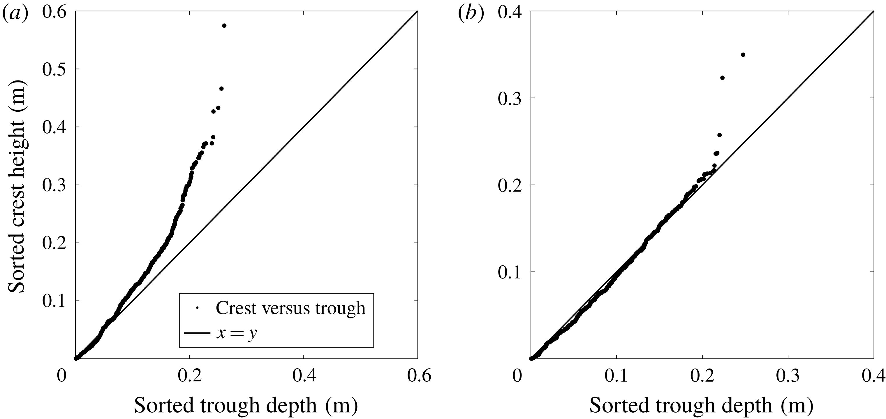
Figure 16. Order statistics for crest and troughs for (a) one original time series and (b) linearised time series.
It is clear that there is a strong vertical asymmetry in this sample time series (for instance, stronger than the one presented by Taylor & Williams (Reference Taylor and Williams2004)) as the crest–trough pairs depart from the red line very soon after the beginning and there is a considerable difference between the largest crests and troughs as well. This also suggests that the Lake George dataset contains many records with very high nonlinearity.
As for the difference between crests and troughs after the linearisation process in figure 16(b), the sorted crest–trough pairs roughly follow the guide line except for several of the largest pairs. Thus the Stokes expansion (A 1) is still valid for extreme cases and the linearisation processes described in the previous subsection are acceptable.


