


1. Introduction
Rayleigh–Bénard convection (RBC), which refers to a layer of fluid confined between parallel horizontal plates and heated from below, is the ideal system for studying convection occurring in both natural and engineering processes (see, e.g. Brent, Voller & Reid Reference Brent, Voller and Reid1988; Hunt & Linden Reference Hunt and Linden1999; Marshall & Schott Reference Marshall and Schott1999; Rahmstorf Reference Rahmstorf2000; Hartmann, Moy & Fu Reference Hartmann, Moy and Fu2001). RBC is determined by the Rayleigh number  $Ra=\alpha g\Delta L^3/\kappa \nu$ and the Prandtl number
  $Pr=\nu /\kappa$, where
  $\alpha$ is the isobaric thermal expansion coefficient,
  $g$ is the gravitational constant of acceleration,
  $\varDelta$ is the temperature difference between the plates,
  $L$ is the spacing between the plates,
  $\kappa$ is the thermal diffusivity coefficient and
  $\nu$ is the kinematic viscosity. In addition, because physically realisable studies use cells with a finite lateral extent, the aspect ratio
  $\varGamma \equiv D/L$ of the sample is another relevant parameter, where
  $D$ is the lateral size of the sample, for instance, the diameter of a cylindrical cell.
The global response of a system to a thermal driving force is reflected in the vertical transport of heat from the bottom plate to the top plate, and such transport is expressed in dimensionless form by the Nusselt number  $Nu=\lambda _{eff}/\lambda$, where the effective conductivity
  $\lambda _{eff}$ is given by
  $\lambda _{eff}=QL/({\rm \pi} (D/2)^2\varDelta )$, with
  $Q$ being the heat flux and
  $\lambda$ being the thermal conductivity of the quiescent fluid. Another parameter that reflects the system response is the extent of turbulence, expressed in terms of a characteristic velocity amplitude
  $U$. Turbulent RBC can also be described by the dimensionless Reynolds number
  $Re=UL/\nu$.
The Nusselt number is equal to 1 when the driving force determined as Ra is small enough and heat is only transferred by the pure conduction of fluid. When  $Ra>Ra_c$, where
  $Ra_c$ is the critical value that represents the onset of convection, convective flows form a pattern and contribute to heat transport. In theory the value of
  $Ra_c$ was calculated by Jeffreys (Reference Jeffreys1928) and found to be 1708 for a sample of infinite lateral extent and with rigid isothermal boundary conditions at the top and bottom plates. This bifurcation was also predicted to be supercritical (Jeffreys Reference Jeffreys1928; Schlüter, Lortz & Busse Reference Schlüter, Lortz and Busse1965). The
  $Nu$ increases continuously and linearly as
  $Ra$ exceeds
  $Ra_c$. This was confirmed with high resolution by numerous experiments. The pattern formation is an interesting aspect of RBC, which has been studied extensively in the sample of large
  $\varGamma ({>}5)$ and at low
  $Ra({<}10^5)$.
As Ra further increases, the flow inside RBC is so strong that it is considered as turbulent convection (Ahlers Reference Ahlers2009; Ahlers, Grossmann & Lohse Reference Ahlers, Grossmann and Lohse2009; Lohse & Xia Reference Lohse and Xia2010), which is mainly studied in small  $\varGamma$(
 $O$(1) or less) samples and characterised by high
  $Ra$ (up to
  $10^{17}$). The turbulent fluid flow in RBC for
  $Ra>10^6$ experiences considerable fluctuation but tends to become organised into a single convection roll or possibly two rolls (with one located above the other) when temporally averaged (see Xi & Xia (Reference Xi and Xia2008), Weiss & Ahlers (Reference Weiss and Ahlers2011) and references therein). The convection rolls in turbulent convection are called large-scale circulation (LSC); it has attracted much attention because it is generally believed to have some connection with (and is statistically similar to) the flow within the Earth's atmosphere (Brown, Nikolaenko & Ahlers Reference Brown, Nikolaenko and Ahlers2005a). The LSC has many intriguing dynamic features, such as azimuthal rotations and occasional cessations and reversals (Sreenivasan, Bershadski & Niemela Reference Sreenivasan, Bershadski and Niemela2002; Brown et al. Reference Brown, Nikolaenko and Ahlers2005a; Xi & Xia Reference Xi and Xia2007; Brown & Ahlers Reference Brown and Ahlers2008b). Over the years, the dynamics of LSC has been extensively studied both experimentally and numerically for wide ranges of
  $Ra$ and
  $Pr$ in two-dimensional/quasi-two-dimensional systems (Sugiyama et al. Reference Sugiyama, Ni, Stevens, Chan, Zhou, Xi, Sun, Grossmann, Xia and Lohse2010; Chandra & Verma Reference Chandra and Verma2011, Reference Chandra and Verma2013; Yanagisawa et al. Reference Yanagisawa, Yamagishi, Hamano, Tasaka and Takeda2011; Ni, Huang & Xia Reference Ni, Huang and Xia2015), cubic or box geometries (Wagner & Shishkina Reference Wagner and Shishkina2013; Foroozani et al. Reference Foroozani, Niemela, Armenio and Sreenivasan2017) and cylindrical cells (Mishra et al. Reference Mishra, De, Verma and Eswaran2011; Sakievich, Peet & Adrian Reference Sakievich, Peet and Adrian2016; Mamykin et al. Reference Mamykin, Kolesnichenko, Pavlinov and Khalilov2018).
The oscillation of the temperature field (Xi et al. Reference Xi, Zhou, Zhou, Chan and Xia2009) in a cylindrical configuration with unity aspect ratio was found to originate from a sloshing mode at the cell centre (Zhou et al. Reference Zhou, Xi, Zhou, Sun and Xia2009) and a torsional mode near the top and bottom plates (Funfschilling, Brown & Ahlers Reference Funfschilling, Brown and Ahlers2008). Motivated by this discovery, Brown & Ahlers (Reference Brown and Ahlers2008b) proposed a stochastic model that could explain the origin of sloshing and torsional oscillations in turbulent convection. This model was subsequently extended by Brown & Ahlers (Reference Brown and Ahlers2008a) by including various perturbations that break the rotational invariance of the sample. An important prediction of this model is the relation between the time-averaged flow strength  $\delta$ and
  $Re$.
$Re$.
Although the results of experiments on LSC in RBC with different geometries (Bai, Ji & Brown Reference Bai, Ji and Brown2016; Ji & Brown Reference Ji and Brown2020) and different  $Pr$ (Xie, Wei & Xia Reference Xie, Wei and Xia2013) are consistent with the predictions from the aforementioned stochastic model, experimental measurements of the LSC strength for low
  $Pr$ (
 $Pr<1$) are still scarce. In experiments at low
  $Pr$, compressed gases at ambient temperature (
 $Pr\sim 1$)(Weiss, Wei & Ahlers Reference Weiss, Wei and Ahlers2016), cryogenic helium (Musilová et al. Reference Musilová, Kréalíík, La Mantia, Macek, Urban and Skrbek2017) and liquid metal (
 $Pr\sim 10^{-3}$) (Mamykin et al. Reference Mamykin, Kolesnichenko, Pavlinov and Khalilov2018; Vogt et al. Reference Vogt, Horn, Grannan and Aurnou2018) were typically used as the working fluid, and a steel sidewall was used to confine the fluid. However, a steel sidewall has such a large thermal conductivity that embedded thermistors cannot detect the temperature reflecting the LSC. Hence, in the present investigation, we explore the LSC in gaseous RBC with
  $Pr=0.72$, and we accomplish this by using a Plexiglas wall.
As Ra increases, an ‘ultimate regime’ is proposed to exist. In the ultimate regime, the flow is dominated by homogenous turbulence and a turbulent boundary layer. Related to the existence of the ultimate regime is whether a coherent LSC continues to exist at very large Ra, or whether it is totally overwhelmed by fluctuations. To better understand this issue, it is of importance to understand the origin of LSC. Previous studies have discussed whether LSC evolves from the well-known cellular structures at low  $Ra$. On one hand, Krishnamurti & Howard (Reference Krishnamurti and Howard1981) performed experiments from which they concluded that LSC is not a simple reflection or continuation of the roll structure observed just after the onset of convection. On the other hand, an explicit search for the mode reported by Krishnamurti & Howard (Reference Krishnamurti and Howard1981) was not successful; see the reviews by Busse (Reference Busse2003) and Hartlep, Tilgner & Busse (Reference Hartlep, Tilgner and Busse2005), who concluded that the LSC at large
  $Ra$ is indeed a reminder of the structures at low
  $Ra$. However, the experiment and simulation in the previously mentioned studies were conducted on RBC samples with a square cross-section, in which the LSC cannot be quantified simply by a temperature measurement, and in Krishnamurti & Howard (Reference Krishnamurti and Howard1981), shadowgraphs were used to capture the flow structure. In the present work, two RBC samples with a circular cross-section and
  $\varGamma =1$ are used, and compressed nitrogen is used as the working fluid. The
  $Ra$ of the experiment ranges from
  $10^{3}$ to
  $10^{9}$, and thus, the flow can be divided into conduction, convection, oscillation, chaotic, transition, and soft and hard turbulent regimes (Threlfall Reference Threlfall1975; Heslot, Castaing & Libchaber Reference Heslot, Castaing and Libchaber1987). Such an
  $Ra$ range permits us to determine whether the LSC in the turbulent regime evolves from cellular structures in the convection regime.
One advantage of this sample is that in such a geometry, the cellular pattern and the LSC constitute a single roll. Fortunately, the strength and azimuthal orientation of a single roll can be determined by the temperature measured from the wall experimentally (Brown, Funfschilling & Ahlers Reference Brown, Funfschilling and Ahlers2007; Xi & Xia Reference Xi and Xia2008; Xie et al. Reference Xie, Wei and Xia2013). Hence, in the present study, we focus on a cylindrical sample with unity aspect ratio  $\varGamma =1$ and a finite-conductivity sidewall, which can have a decisive influence on the convective pattern, and we measure the temperature in the wall to directly compare the cellular pattern with the LSC. At small
  $\varGamma \leqslant 1.6$, the cellular pattern reported by Stork & Müller (Reference Stork and Müller1975) and Müller, Neumann & Weber (Reference Müller, Neumann and Weber1984) is an unstable, non-axisymmetric single convection roll corresponding to an azimuthal Fourier mode with
  $m=1$. This pattern was further confirmed by Hébert et al. (Reference Hébert, Hufschmid, Scheel and Ahlers2010), who used the shadowgraph technique and a direct numerical simulation (DNS) to study the aforementioned cellular pattern near the critical Rayleigh number
  $Ra_c$. The
  $Ra_c$ values in cylindrical samples of fairly small
  $\varGamma$ have been studied by several theoretical investigations (Charlson & Sani Reference Charlson and Sani1970, Reference Charlson and Sani1971; Buell & Catton Reference Buell and Catton1983). Among them, only the linear stability analysis extended by Buell & Catton (Reference Buell and Catton1983) included the effect of the finite sidewall conductivity and applied rigid isothermal boundary conditions to the top and bottom of the domain. Moreover, the marginal stability curves were given for several wall admittances
  $C\equiv [(D/2)\lambda ]/(d_w\lambda _w)$, where
  $d_w$ is the thickness and
  $\lambda _w$ is the thermal conductivity of the sidewall. However, the
  $Ra_c$ for a finite
  $C$ and
  $\varGamma =1$ has not been determined experimentally.
In the present paper,  $Ra_c$ is reported to be 7300 for
  $Pr=0.72$ and a finite wall admittance
  $C=2.02$. In an experiment, the
  $\delta$ values of the cellular pattern and LSC are measured as a function of
  $Ra$, revealing a sharp sequence change as a function of
  $Ra$. The flow strength of the cellular pattern exhibits sharp growth with
  $Ra$ in the convection regime, a sudden decrease in the chaotic regime and a further decrease in the transition regime. When
  $Ra$ is further increased and the RBC evolves into the soft turbulence regime, the LSC becomes self-organised, and the flow strength exhibits sharp growth with
  $Ra$. Then, the flow strength decreases as
  $Ra$ increases in the hard turbulence regime. The dependence of the LSC on
  $Ra$ is similar to that of the cellular pattern on
  $Ra$, suggesting that LSC is an analogy with a cellular pattern. This finding also indicates that the
  $\delta$ of the LSC will further decrease when
  $Ra$ is larger than that in the present work. Furthermore, a comparison between the present work and previous LSC results for larger
  $Ra$ and large
  $Pr$ is made, revealing more sharp changes of the flow strength of the LSC with
  $Ra$. Although the flow strength of the LSC is similar to that of the cellular pattern, the preferred orientation of both structures shows a phase difference. In the soft and hard turbulent regimes,
  $Re$ is also obtained for
  $Pr=0.72$, and the result is inconsistent with those of previous studies, and with the prediction from the model by Brown & Ahlers (Reference Brown and Ahlers2008b) for
  $Pr>3$.
The remainder of this paper is organised as follows. In § 2, we introduce the experimental apparatus, the properties of the fluid used in the experiments and the experimental procedure. In § 3, we present the results regarding the transport of heat and flow strength, we also describe the method used to extract  $Ra$ between several regimes, and the
  $Re$ of the LSC is presented. In § 4, we discuss our results and compare them with those of other experiments. The paper finishes with a brief summary in § 5.
2. Apparatus and procedures
2.1. The apparatus
The experiments were conducted with two different sets of convection apparatus, with similar features. The features were described before by Wan et al. (Reference Wan, Wei, Verzicco, Lohse, Ahlers and Stevens2019), but we describe the apparatus in detail here. A schematic diagram is provided in figure 1. From bottom to top, the apparatus consisted first of a bottom adiabatic shield (A) made of aluminium. The central area of the bottom of part A, with a diameter of 25.4 cm, was covered uniformly by parallel straight grooves with a depth of 0.76 cm and a width of 0.40 cm, which were interconnected by semicircles at their ends. Adjacent grooves were separated by a spacing of 1.9 cm. Epoxied into the grooves was a heater made of American Wire Gauge No. 15 nichrome C resistance wire surrounded by fibreglass sleeving.
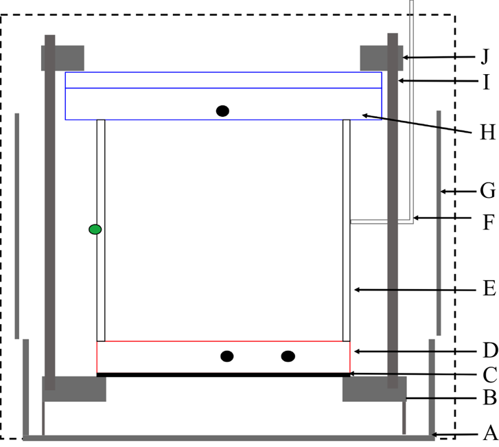
Figure 1. A diagram of an RBC cell. The various parts are explained in the text. The black circles on the top and bottom copper conducting plates represent the embedded thermistors. The green circle in the Plexiglas wall represents a thermistor embedded in a blind hole (without penetrating the wall).
Suspended above the shield on a steel cylinder  $3.8$ cm high with a wall thickness of
  $0.32$ cm was the bottom supporting bracket (B) made of aluminium, with a thickness of
  $3.5$ cm. The bottom plate (D) of the sample sat directly above the inner edge of part B. The bottom plate was made of oxygen-free high-conductivity copper with a thickness of 5.08 cm; its top surface was finely machined with tool marks of depth less than
  $3 \ \mathrm {\mu }\textrm {m}$. The bottom surface was attached to an adhesive film heater (C) (Omega, model KHRA-8/2-P), which had a diameter of
  $20.3$ cm and a resistance of 25.63
  $\varOmega$. The bottom plate's diameter was
  $22.2$ cm, while the central section had a reduced diameter of 20.3 cm and was 0.8 mm thinner than the edge so that the Plexiglas sidewall cylinder (E) was a close sliding fit into the bottom plate. Between parts D and E, an ethylene-propylene O-ring (Parker, model 2-171) was placed in a groove carved into the top surface of the bottom plate; this O-ring prevented the leakage of gas. One small hole was drilled horizontally from the side to the centre of the bottom plate, while a second hole was drilled to
  $1/2$ of the radius. Thermistors were placed inside a hollow copper tube and embedded into these holes at a vertical distance of 2.53 cm from the top surface of the bottom plate.
The inner diameter  $D$ of the Plexiglas sidewalls was measured at several angular and axial positions, and the standard deviation from the measurement mean for a particular sidewall was generally
  $0.03$ cm with a mean
  $D$ of
  $19.05$ cm. The wall thickness was 0.63 cm. The wall length
  $L$ was equal to
  $D$ and was uniform around the circumference to within
  ${\pm }0.01$ cm. A thin Teflon capillary (F) penetrated the sidewall at mid-height and was used to fill the cell. Externally, the capillary was connected to a fill line coming from the gas supply cylinder, to a pressure gauge (Paroscientific Model 745) and to another volume known as the hot volume (HV) (Mueller, Ahlers & Pobell Reference Mueller, Ahlers and Pobell1976). The HV had a size similar to that of the cell, and its temperature was adjusted in a feedback loop with the pressure gauge to keep the sample pressure constant. The HV is not shown in figure 1.
The sidewall was surrounded by an adiabatic side shield (G) made of aluminium. Epoxied to the outside of this shield was a double spiral of aluminium tubing, through which water from a temperature-controlled circulator flowed. The shield was suspended by six plastic rods above the supporting plate of a rotating table; the supporting plate of the rotating table and the rods are not shown in figure 1. During the measurements, the temperature of the shield was kept close to the mean temperature of the system.
The top of the sample was composed of a copper plate (H) with a diameter of 25.4 cm. This diameter of 25.4 cm was originally designed for the top plate for experimental purposes, as reported by Brown et al. (Reference Brown, Nikolaenko, Funfschilling and Ahlers2005b). Here, the central section of the top plate was 20.32 cm in diameter and 0.8 mm thinner than the edge. An O-ring was also placed in the groove carved on the bottom surface of the top plate, similar to that in the bottom plate. The top plate had a thickness of 3.34 cm, and a double-spiral water-cooling channel was machined directly into the plate. Small holes were drilled from above through the two-plate composite to within 0.32 cm of the copper–fluid interface, and calibrated thermistors were mounted into the holes; these thermistors were protected from circulating water by an additional small O-ring between the two plates. In the present work, one thermistor was placed in the centre of the top plate to record the temperature of the top plate. In the top, a retaining aluminium bracket (J) and six tension rods (I) were provided to sustain the force exerted by pressures reaching up to 10 bar. To prevent the convection of air in the vicinity of the sample, the entire space outside the sample, but inside the dashed rectangle K was filled with a low-density (firmness rating 1) polyurethane foam sheet. During the experiment, the whole apparatus was levelled to less than  $10^{-4}$ rad.
2.2. Temperature measurement
Two different sidewalls were used in the present work. The first wall (A) had three layers of eight temperature probes embedded in holes on (but not penetrating) the sidewall. The second wall (B) had only one layer of eight temperature probes around the sidewall but six smaller thermistors penetrating the wall into the fluid. In cell A only the temperatures at the mid-height layer were analysed. In cell B only the power spectrum of temperature of one thermistor was analysed. The location of this thermistor was  $\xi \equiv (1-r/(D/2)) = 0.063$ and
  $z/L= 0.51$, where
  $r$ is the distance from the axis of the sample and
  $z$ is the vertical distance from the surface of the bottom plate. In the present work, the side thermistor in cell B was placed around the LSC plane. The Nusselt number, flow strength and Fourier energy were measured mostly from cell A, in which the fluid was not affected by any thermistor. However, with regard to
  $Re$, the measurement was made from cell B.
Except for those on the sidewalls and inside the fluid, the thermistors used in the apparatus were calibrated simultaneously in a separate apparatus against a laboratory standard based on a standard platinum thermometer. Deviations of the data from the fit were generally less than  $0.002\,^\circ \textrm {C}$. The thermistors were mounted on the adiabatic bottom shield, adiabatic side shield, bottom plate, top plate and bottom aluminium bracket. In contrast, the thermistors embedded on the walls and inside the fluid were calibrated against the top- and bottom-plate thermistors after being installed in the sidewall and inside the fluid. During the calibration, the plate temperatures were set such that
  ${\varDelta =0.1\,^\circ \textrm {C}}$ to ensure that the cell was in equilibrium for more than 12 h. The thermistors in the sidewall and inside the fluid were then assumed to be at the mean temperature
  $T_m$ of the top and bottom plates. The deviation of the data from the fit was less than
  $0.01\,^\circ \textrm {C}$.
2.3. The fluid
Nitrogen was used as the working fluid, and nearly all of the measurements were made with a mean temperature of  $25.00\,^\circ \textrm {C}$. Although various physical properties, such as the thermal expansion coefficient
  $\alpha$, thermal diffusivity
  $\kappa$ and kinematic viscosity
  $\nu$, depend on the pressure and mean temperature, the nitrogen gas used in the present work yielded a constant
  $Pr$ at different pressures, as demonstrated in figure 2. Another relevant property is the thermal conductivity
  $\lambda$, which gives a value of wall admittance
  $C\equiv \lambda (D/2)/(\lambda _{w}d_{w})$ (where
  $\lambda _w=0.192\ \textrm {W}\ \textrm {m}^{-1}$ K is the thermal conductivity of the sidewall and
  $d_w$ is the thickness of the sidewall). The wall admittance for RBC with nitrogen at
  $25.00\,^{\circ }\textrm {C}$ was found to be
  $2.02$.

Figure 2. (a) A diagram of the gas pressure  $P$ and temperature drop
  $\varDelta$ between two convection cells. (b) A diagram of
  $Pr$ vs.
  $Ra$. In (a,b), the open symbols represent convection cell A without thermistors disturbing the flow, while the solid symbols represent convection cell B with thermistors inside the fluid.
2.4. Experimental procedure
The temperatures of the top and bottom plate were regulated to maintain a constant value at first. Then, the convection cell and the HV were evacuated by a diffusion pump. Nitrogen at a pressure of 10 bar was injected into the convection cell in order to flush the system. Later, the convection cell was re-evacuated. The cell was again flushed with nitrogen to ensure that there were no other gas molecules inside. After being evacuated a third time, the convection cell was filled with nitrogen to a pressure close to the desired value. Then, the valve between the HV and the gas cylinder was closed. The pressure of both the HV and the convection cell was maintained by regulating the temperature of the HV. While the temperature drop and the pressure of the convection cell were maintained at given values, the temperatures of the probes in the convection cell were collected simultaneously. For the next pressure increment, more nitrogen was pumped into the convection cell, and the above procedure was repeated.
During a typical experimental run, at a constant  $\varDelta$ and pressure
  $P$, all thermistors were read every 4 s or so for at least 10 h. To evaluate the data, the readings from the first few hours were discarded to avoid transients. Because only the pressure changed slightly between two successive experiments, it was usually sufficient to discard only the first hour of data. In cell B, the thermistors outside the fluid were measured in the same way as the thermistors in cell A. However, each of the six thermistors inside the fluid was connected to an individual multimeter, and data were collected at a rate of 16.6 Hz. In cell B, a given run at equilibrium typically lasted more than 36 h.
3. Results
3.1. A single-roll structure
3.1.1. Quantitative measurements of a single-roll structure
The strength  $\delta$ and azimuthal orientation
  $\theta _0$ of a single-roll structure can be determined by fitting eight temperatures, denoted
  $T_{i}$ (
 $i=0,\ldots ,N_T-1$, where
  $N_T=8$ is the number of thermistors around the sidewall), around the sidewall with the following equation:
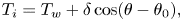 \begin{equation} T_{i}=T_w+\delta \cos(\theta-\theta_0), \end{equation}
where  $T_{i}$ denotes the temperature located at azimuthal location
  $\theta$. Here
  $\theta$ is in the range
  $-{\rm \pi} \leqslant \theta <{\rm \pi}$. Generally, the above equation fits the instantaneous temperature profile well, as shown in figure 3(a). However, if the single-roll structure breaks down and
  $\delta$ is sufficiently small, the above equation does not effectively fit the instantaneous temperatures. As shown in figures 3(b), 3(c) and 3(d) the temperatures are fitted by the equation
  $T_{i}=T_w+\delta \cos [m(\theta -\theta _0)]$ with a high mode (
 $m>1$, where
  $m$ represents the number of hot/cold spots evenly appearing on the mid-height plane as visualised from particle image velocimetry by Xi et al. Reference Xi, Zhang, Hao and Xia2016). At some
  $Ra$, a single-roll structure does not form. To further quantify the flow structure and make use of all eight temperatures, we computed the coefficients for the lowest four Fourier modes from the
  $N_T$ temperatures
  $T_{i}$ as follows:
 \begin{equation} T_{i} = \sum_{m=0}^{N_T/2} {A_{m}\cos(m\theta)+B_{m}\sin(m\theta)}. \end{equation}
Figure 3. Examples of temperature profiles measured by sidewall thermistors on the mid-height plane. The measurements were taken at  $Ra=6.4\times 10^6$ and
  $Pr=0.72$ in cell A with nitrogen as the working fluid. In (a), (b), (c) and (d) the dashed lines represent the fitting by the equation
  $T=T_{w}+\cos (m(\theta -\theta _0))$ with
  $m=1,2,3$ and
  $4$, respectively. The solid lines represent the fitting by (3.2).
The above yielded all eight Fourier coefficients  $A_{m}$ (the cosine coefficients) and
  $B_{m}$ (the sine coefficients),
  $m=1,\ldots ,4$, for the case where there are eight temperatures. From these coefficients, we determined the energy
  $E_m = A^2_m + B^2_m$ for each mode
  $m=1,\ldots ,N_T/2$. Then, the first Fourier energy mode is
  $E_{1} = \delta ^2$, and the orientation of the single-roll structure is given by
  $\theta = \textrm {arctan}(B_1/A_1)$. If the flow structure is a single roll and the horizontal mid-height plane consists of only one hot up-flow and one cold down-flow, (3.1) will apparently fit the temperatures well as shown in figure 3(a), and the ratio
  $E_{1}/E_{tot}$ should be close to 1. However, when the single-roll structure breaks down, the ratio
  $E_{1}/E_{tot}$ vanishes. As shown in figure 3(b), at the dominant higher Fourier energy mode (
 $m=2$), the Fourier energy ratio
  $E_{2}/E_{tot}$ is much larger than that at the other modes. Higher modes
  $m=3$ and
  $m=4$ are dominant in figures 3(c) and 3(d), respectively. Table 1 also lists the total energy and the ratio of each energy mode, in total energy, for the examples in figure 3. The examples are all taken for
  $Ra=6.4\times 10^{6}$ and
  $\varDelta =10.0$ K, but the total Fourier energy in figures 3(b), 3(c) and 3(d) are much smaller than figure 3(a). In figures 3(b), 3(c) and 3(d) the ratio of the first energy mode are all smaller than
  $0.4$.
Table 1. The total Fourier energy  $E_{tot}$, and the ratio of Fourier energy and total energy
  $E_{m}/E_{tot}$ (
 $m=1,\ldots ,4$) for the examples in figure 3.

Next, we examined how the Fourier mode describes the dynamics of the single-roll structure. In figures 4, 5, 6, 7, 8 and 9 the time trace of temperature measured from the sidewall, the corresponding Fourier energy, the flow strength and orientation are plotted for different  $Ra$. Apparently the total Fourier energy gives a similar trend as the flow strength for most of
  $Ra$. When
  $Ra$ is large enough, the flow strength varies drastically as time changes. In turbulent RBC, at a given Ra the LSC strength
  $\delta \sim 0$ corresponds to a process called cessation, during which the LSC breaks down owing to the strong stochastic turbulent background. If the flow strength
  $\delta <\beta \langle \delta \rangle$, cessation occurs. However, the selection of
  $\beta$ is quite arbitrary in the previous literature. Furthermore, the aforementioned criteria for cessation are not applicable when cessation is the most common state of flow and the time-averaged flow strength
  $\langle \delta \rangle$ is nearly 0, as shown in figure 7 for
  $Ra=6.4\times 10^{6}$. Here, we proposed that
  $E_{1}/E_{tot} < 0.4$ can be used as the criterion of cessation. In figure 8(e), the minimum value of the first energy mode takes up more than
  $0.4$ total energy, therefore there is no cessation at this
  $Ra$. Using the ratio
  $E_{m}/E_{tot}$, it is easier to determine the order of the mode dominating the flow that breaks down the single-roll structure. To better illustrate this technique, the time traces of
  $E_{tot}$ and each ratio
  $E_{m}/E_{tot}$ were also plotted in figure 7(c,d). At
  $Ra=6.4\times 10^{6}$, the flow structure does not form even a single roll, as
  $E_{1}/E_{tot}$ is mainly less than 0.5. Surprisingly, the dominant Fourier mode at this
  $Ra$ is
  $m=4$, whose energy takes up to more than half of the total Fourier energy. In a later section, the time-averaged values and standard deviations of the flow strength
  $\delta$ and orientation
  $\theta _0$ will be analysed in addition to the ratio of each Fourier mode
  $E_{m}/E_{tot}$ (
 $m=1,\ldots ,4$).
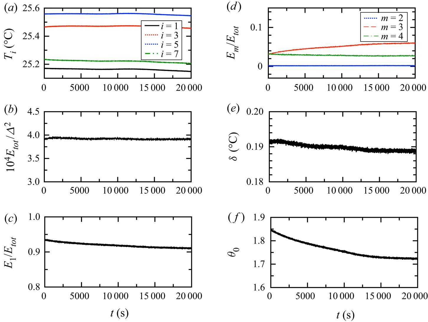
Figure 4. The time trace of various quantities for convection regime with  $Ra=8.5\times 10^4$. (a) The four temperatures measured at mid-height. (b) The total Fourier energy
  $10^4E_{tot}/\varDelta ^2$. (c) The ratio of the first Fourier energy mode and total energy
  $E_1/E_{tot}$. (d) The ratio
  $E_{m}/E_{tot}$ with
  $m=2$, 3 and 4. (e) The flow strength
  $\delta$. (f) The LSC orientation
  $\theta$.

Figure 5. The time trace of various quantities for oscillation regime with  $Ra=1.5\times 10^5$. (a) The four temperatures measured at mid-height. (b) The total Fourier energy
  $10^4E_{tot}/\varDelta ^2$. (c) The ratio of the first Fourier energy mode and total energy
  $E_1/E_{tot}$. (d) The ratio
  $E_{m}/E_{tot}$ with
  $m=2$, 3 and 4. (e) The flow strength
  $\delta$. (f) The LSC orientation
  $\theta$.

Figure 6. The time trace of various quantities for the chaotic regime with  $Ra=4.7\times 10^5$. (a) The four temperatures measured at mid-height. (b) The total Fourier energy
  $10^4E_{tot}/\varDelta ^2$. (c) The ratio of the first Fourier energy mode and total energy
  $E_1/E_{tot}$. (d) The ratio
  $E_{m}/E_{tot}$ with
  $m=2$, 3 and 4. (e) The flow strength
  $\delta$. (f) The LSC orientation
  $\theta$.

Figure 7. The time trace of various quantities for the transition regime with  $Ra=6.4\times 10^6$. (a) The four temperatures measured at mid-height. (b) The total Fourier energy
  $10^4E_{tot}/\varDelta ^2$. (c) The ratio of the first Fourier energy mode and total energy
  $E_1/E_{tot}$. (d) The ratio
  $E_{m}/E_{tot}$ with
  $m=2$, 3 and 4. (e) The flow strength
  $\delta$. (f) The LSC orientation
  $\theta$.

Figure 8. The time trace of various quantities for the soft turbulence regime with  $Ra=1.4\times 10^7$. (a) The four temperatures measured at mid-height. (b) The total Fourier energy
  $10^4E_{tot}/\varDelta ^2$. (c) The ratio of the first Fourier energy mode and total energy
  $E_1/E_{tot}$. (d) The ratio
  $E_{m}/E_{tot}$ with
  $m=2$, 3 and 4. (e) The flow strength
  $\delta$. (f) The LSC orientation
  $\theta$.

Figure 9. The time trace of various quantities for the hard turbulence regime with  $Ra=1.1\times 10^8$. (a) The four temperatures measured at mid-height. (b) The total Fourier energy
  $10^4E_{tot}/\varDelta ^2$. (c) The ratio of the first Fourier energy mode and total energy
  $E_1/E_{tot}$. (d) The ratio
  $E_{m}/E_{tot}$ with
  $m=2$, 3 and 4. (e) The flow strength
  $\delta$. (f) The LSC orientation
  $\theta$.
3.1.2. Convective pattern and large-scale circulation
We first examined the Rayleigh number range where the cellular pattern and the LSC exist separately. Figure 10(a) shows plots of the flow strength  $\langle \delta \rangle /\varDelta$ as a function of
  $Ra$ with
  $Pr=0.72$ and nitrogen as the working fluid. Obviously, the data show a sequence of discontinuities. By fitting the data with several logarithmic functions, the transitions between six regimes are determined (except the oscillation regime, which is determined by the power spectrum of the temperature embedded in the sidewall). These seven regimes, namely, conduction, convection, oscillation, chaotic, transition, soft turbulence and hard turbulence, are consistent with those reported by Heslot et al. (Reference Heslot, Castaing and Libchaber1987). In the present case, the
  $Ra$ of the transitions between these seven different regimes are denoted
  $Ra_c$,
  $Ra_{o}$,
  $Ra_{ch}$,
  $Ra_{tr}$,
  $Ra_{s}$ and
  $Ra_{h}$ with values of
  $7300$,
  $1.35\times 10^5$,
  $1.65\times 10^5$,
  $6.14\times 10^5$,
  $8.38\times 10^6$ and
  $9.18\times 10^7$, respectively. Hence, the
  $Ra$ between the transitions can also be expressed as
  $Ra_{o}=18.5Ra_c$,
  $Ra_{ch}=22.6Ra_c$,
  $Ra_{tr}=84Ra_{c}$,
  $Ra_{s}=1148Ra_{c}$,
  $Ra_{h}=12\,575Ra_c$.

Figure 10. Plots of (a) the single-roll flow strength  $\langle \delta \rangle /\varDelta$ and (b)
  $\sigma _\delta /\varDelta$ against
  $Ra$ for cell A. Six dynamical states are labelled. From left to right, they are (I) convection, (II) conduction, (III) chaotic, (IV) transition, (V) soft turbulence and (VI) hard turbulence. The dashed lines are logarithmic function fits to various segments of data serving as visual guides. The vertical lines from left to right are as follows:
  $Ra_c=7300$,
  ${Ra_{ch}=1.85\times 10^{5}}$,
  $Ra_{tr}=6.14\times 10^{5}$,
  $Ra_{s}=8.38\times 10^{6}$ and
  $Ra_{h}=9.18\times 10^{7}$. (Here, the oscillation regime between the corresponding
  $Ra_{o}=1.35\times 10^{5}$ and
  $Ra_{ch}$ is not shown.) The measurements were taken from cell A for
  $\varDelta = 4.00$ K (black circles) and
  $\varDelta = 10.00$ K (red squares).
In the conduction regime,  $\langle \delta \rangle /\varDelta$ has a value of
  $0.0047$, close to but still greater than 0. This measurement was taken at
  $\varDelta =4.00\ \textrm {K}$, so it yields a temperature difference of nearly 20 mK, which is only twice the measurement error. Thus, we consider this as the measurement error. As
  $Ra$ is increased beyond
  $Ra_c$, the strength of the cellular pattern sharply increases and reaches a maximum
  $0.02$ in the convection regime. A sharp increase in cellular strength was also observed by Hébert et al. (Reference Hébert, Hufschmid, Scheel and Ahlers2010), who used the shadowgraph image variance
  $\sigma ^2$ to determine
  $Ra_c$. Those authors found that
  $\sigma ^2$ experiences linear growth with
  $Ra$ when
  $Ra$ is just greater than
  $Ra_c$, a similar trend to that of the Nusselt number. Therefore, we also expected a linear increase in
  $\langle \delta \rangle /\varDelta$ with
  $Ra^{1/2}$ because the first Fourier energy is
  $\delta ^2$ as mentioned previously. Although we obtained only a few data points at the onset of convection, they are sufficient to fit function
  $\langle \delta /\varDelta \rangle =k(Ra-Ra_c)^{1/2}+b$ to obtain
  $Ra_c=7300$. We note that the
  $Ra_c$ value determined by a logarithmic function is close to 7300 in figure 18 in Appendix A.
The oscillation regime cannot be determined from the relation between the flow strength and  $Ra$, so we will discuss the oscillation regime in a later section. As
  $Ra$ increases up to
  $Ra_{ch}$, the strength of a single roll varies over time. From figure 10(b), we can see that the fluctuation in the flow strength increases as
  $Ra$ is increased in the chaotic regime. However, the flow with the
  $m=1$ mode is still dominant in the chaotic regime, as shown in figure 11. The energy ratio
  $E_{1}/E_{tot}>0.75$ means that the flow always forms a single roll in the cell. This single-roll flow usually meanders around a preferred orientation, as shown in figure 12, where the time-averaged orientation
  $\langle \theta \rangle \sim 2$ rad, but the fluctuation in the orientation
  $\sigma _\theta$ is approximately
  $0.15$ rad. In the transition regime
  $Ra>Ra_{tr}$, the time-averaged flow strength continues to decrease to the value in the conduction regime, which represents the resolution of the experimental measurement. For a given
  $Ra$, the flow strength of the single-roll structure varies temporally, as demonstrated in figures 4, 6, 7, 8 and 9. To ascertain whether the single-roll flow retains its shape, the time trace of the ratio
  $E_{m}/E_{tot}$ in transition regime is also plotted in figure 7(c), indicating that the single-roll flow breaks down and then reforms itself during the measurement period. When the
  ${m=1}$ single-roll flow vanishes, the strong background fluctuation represented by the
  $m=4$ mode in the present measurement is dominant. In the transition regime, the ratio
  $E_4/E_{tot}$ is comparable with
  $E_1/E_{tot}$. Another difference between the chaotic and transition regimes also lies in the correlation between the temperature in the centre and the temperature near the sidewall; this correlation is not shown in the present work because it is consistent with the previous measurements by Heslot et al. (Reference Heslot, Castaing and Libchaber1987). In the chaotic regime, the temperatures in the centre and near the sidewall are strongly correlated. Once the flow changes to the transition regime, this correlation disappears.

Figure 11. The ratios of the  $m$th mode of Fourier energy to the total Fourier energy
  $E_{m}/E_{tot}$ (
 $m=1,\ldots ,4$) against
  $Ra$. The vertical lines represent the transitions between different dynamic regimes. The measurements were taken from cell A for
  $\varDelta = 4.00\ \textrm {K}$ (black circles) and
  $\varDelta = 10.00\ \textrm {K}$ (red squares).

Figure 12. (a) The time-averaged orientation  $\langle \theta \rangle$ and (b) the standard deviation
  $\sigma _\theta$ of the LSC against
  $Ra$. The vertical lines represent the transitions between different dynamic regimes. The measurements were taken from cell A for
  $\varDelta = 4.00\ \textrm {K}$ (black circles) and
  $\varDelta = 10.00\ \textrm {K}$ (red squares).
As  $Ra$ is further increased to the soft turbulence regime, a single-roll LSC is observed. As
  $Ra$ increases, the time-averaged flow strength
  $\langle \delta \rangle /\varDelta$ increases sharply, but the standard deviation of the flow strength
  $\sigma _{\delta }/\varDelta$ also decreases drastically. The maximum LSC strength is 50 % larger than the maximum value of the cellular pattern strength. The corresponding onset of turbulence at
  $Ra_{s}=8.38\times 10^{6}$ was determined from fitting a logarithmic function to the time-averaged flow strength
  $\langle \delta \rangle /\varDelta$ against
  $Ra$. However, if the time-averaged flow strength is fitted by the function
  $\langle \delta /\varDelta \rangle =k(Ra-Ra_s)^{1/2}+b$, the value of
  $Ra_{s}$ is still close to
  $8.38\times 10^{6}$, as shown in figure 18 in Appendix A. Interestingly, the single-roll LSC is stronger under a more turbulent background, which is represented by
  $Ra$. However, in the hard turbulence regime, the strength of the LSC decreases as
  $Ra$ increases and the turbulent background becomes stronger. In hard turbulence where
  $Ra>Ra_{h}$, the flow strength
  $\langle \delta \rangle /\varDelta$ slowly decreases as
  $Ra$ increases, and the standard deviation of the flow strength
  $\sigma _{\delta }$ is close to 0, which means that the strength of the LSC is barely affected by the turbulent background.
The growth of the LSC strength with  $Ra$ is similar to that of the cellular pattern, suggesting that the LSC reflects low
  $Ra$ structures. However, some interesting differences remain between the cellular pattern and the LSC, as shown in figure 12. It is well known that the single-roll LSC meanders randomly around a preferred orientation
  $\theta _m$, which would be apparent in the probability distribution of the orientation
  $p(\theta _0)$ given sufficient statistical data. However, in present work the measurement of LSC in equilibrium for each Ra only lasts for approximately 8 h, and it is difficult to determine the peak at the probability density function (p.d.f.) of
  $\theta _0$ as shown in figure 13(f) for
  $Ra=1.1\times 10^8$. So here we take the time-averaged orientation
  $\langle \theta _0\rangle$ as a preferred orientation;
  $\theta _0$ would ideally be uniformly distributed in an azimuthally symmetric system, but minor deviations from perfect rotational symmetry such as a slightly elliptical cross-section of the sidewall, a systematic temperature gradient in the top plate owing to the cooling system or a coupling of the Earth's Coriolis force to the LSC (Brown & Ahlers Reference Brown and Ahlers2006) could cause a deviation from the uniform distribution. It is worth noting that the orientation of the cellular pattern has a phase difference of approximately
  ${\rm \pi} /4$ from that of the LSC. In the soft turbulence regime, the relation of
  $\langle \theta \rangle$ against
  $Ra$ shows a smooth change in the flow orientation. In figure 13, the distribution of the orientations are plotted for different
  $Ra$. In the convection regime, the pattern stays at the orientation about
  $\theta =2$. In the oscillation regime, the pattern slowly moves in clockwise direction to the orientation
  $2.6$ in figure 5(f). In the chaotic and transition regimes, the pattern varies over the plates at a range
  $0.5<\theta <3$. In the soft turbulence regime, the LSC meanders about a preferred orientation, and this orientation is smaller with increasing
  $Ra$. In the hard turbulence regime, the preferred orientation of LSC varies little as
  $Ra$ increases. In convection cell A, the cell was levelled within the error of measurement, and the capillary tube was oriented east, which is the preferred orientation of the LSC. If the preferred orientation of the LSC suggests that an imperfect element oriented east was introduced during the experiment, we are surprised to find that the cellular pattern chooses to be
  ${\rm \pi} /4$ away from that imperfect element. More studies comparing cellular patterns with LSC are needed to shed light on this phenomenon.

Figure 13. The p.d.f. distribution of the LSC orientation  $\theta$ for various regimes. (a) Convection regime with
  $Ra=8.5\times 10^4$. (b) Oscillation regime with
  $Ra=1.5\times 10^5$. (c) Chaotic regime with
  $Ra=4.7\times 10^5$. (d) Transition regime with
  $Ra=6.4\times 10^6$. (e) Soft turbulence regime with
  $Ra=1.4\times 10^7$. (f) Hard turbulence regime with
  $Ra=1.1\times 10^8$. The vertical lines represent the azimuthal location
  $\theta =2.0$. The measurements were taken from cell A.
3.2. Reynolds numbers based on the turnover time of large-scale convection
Another difference between cellular patterns and the LSC is that the latter can be described by a unique eddy-turnover time in turbulent context, which is correlated with the oscillation period  $\tau _0$ of the LSC. The oscillation period
  $\tau _0$ was inferred as the oscillation time from the autocorrelation of a single temperature measurement. From the temperature power spectra shown in figure 14, the frequency of the peak
  $f_0$ is equivalent to
  $1/\tau _0$. Therefore, using
  $L$ as a relevant length scale,
  $Re$ can be defined as
 \begin{equation} Re\equiv\frac{2L^2f_0}{\nu}. \end{equation}
Figure 14. (a) The temperature power spectra located at  $\xi =0.063$ and
  $z/L=0.51$ inside fluid of cell B for
  $Ra = 7.75\times 10^7$ (soft turbulence). (b) From bottom to top, the temperature power spectrum located at
  ${\rm \pi} /16$ in the sidewall of cell A for
  $Ra = 1.35\times 10^5$ with
  $\varDelta = 10$ K and for
  $Ra = 1.65\times 10^5$ with
  $\varDelta =4$ K; both
  $Ra$ are in the oscillation regime.
In cell A, the temperatures in the sidewall (except in the oscillation regime) do not show obvious peaks in the temperature power spectra, mainly because the Plexiglas wall used in the present work is twice as thick as the wall used in Brown et al. (Reference Brown, Funfschilling and Ahlers2007). Hence, the oscillation of the temperature owing to the LSC is damped before it is detected by the probe. In convection cell B, which has thermistors inside the fluid, only the power spectra in the soft and hard turbulence regimes show obvious peaks, as indicated in figure 14(a). Because the thermistor near the sidewall inside the fluid is located on the LSC plane, the oscillation peak of the side temperature represents the turnover time of the LSC (Brown et al. Reference Brown, Funfschilling and Ahlers2007).
The LSC turnover time has been studied extensively in a large range of both  $Ra$ and
  $Pr$. For comparison purposes, figure 15 plots our data with those from two other experiments. One set of data is
  $Re^{pl}$, which is also based on the LSC turnover time of Brown & Ahlers (Reference Brown and Ahlers2007) and is taken from RBC with
  $\varGamma =1.00$ and
  $Pr=3.32$,
  $4.38$ and
  $5.55$. The other set is run ‘C’ of Bruno convection taken from RBC with unity
  $\varGamma$ using cryogenic helium gas as the working fluid, yielding
  $Pr\sim 1$. The
  $Pr$ of the experiment with cryogenic helium gas from Musilová et al. (Reference Musilová, Kréalíík, La Mantia, Macek, Urban and Skrbek2017) is close to our
  $Pr$, but there is a discrepancy between the
  $Re_{f_0}$ of our work and that measured with cryogenic helium gas. Figure 15(a) also demonstrates that our LSC turnover time is consistent with that of Brown & Ahlers (Reference Brown and Ahlers2007), who employed a larger
  $Pr$ than ours.
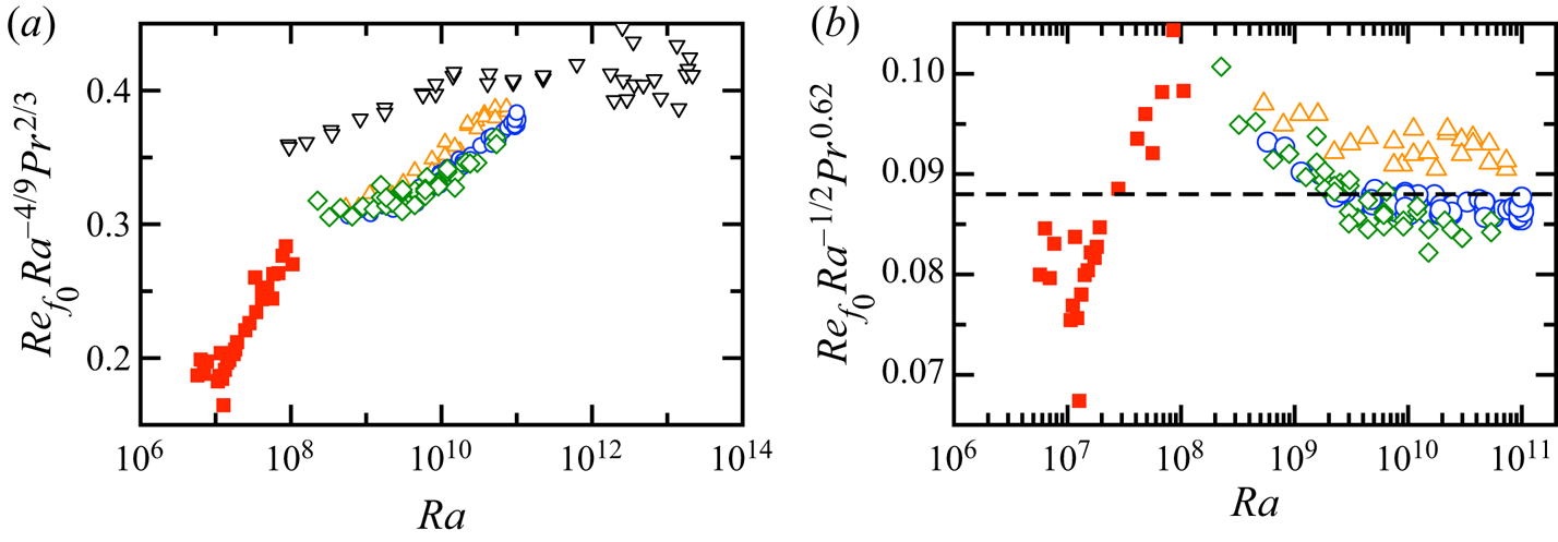
Figure 15. (a) Values of  $Re$ multiplied by
  $Ra^{-4/9}Pr^{2/3}$. Squares, this work, cell B,
  $Pr=0.72$.; black triangles, from Bruno, run ‘C’ of Musilová et al. (Reference Musilová, Kréalíík, La Mantia, Macek, Urban and Skrbek2017),
  $Pr\sim 1$; orange triangles, from Brown et al. (Reference Brown, Funfschilling and Ahlers2007),
  $Pr=3.32$; circles, from Brown et al. (Reference Brown, Funfschilling and Ahlers2007),
  $Pr=4.38$; diamonds, from Brown et al. (Reference Brown, Funfschilling and Ahlers2007),
  $Pr=5.55$. (b)
  $Re_{f_{0}}Ra^{-1/2}Pr^{0.62}$ against
  $Ra$.
$Ra$.
Brown & Ahlers (Reference Brown and Ahlers2008b) proposed a model consisting of two stochastic ordinary differential equations to explain most of the features of LSC dynamics. One important prediction of this model is the relation between the normalised flow strength of the LSC and  $Re$, which is expressed as
 \begin{equation} \frac{\langle\delta\rangle}{\varDelta}\times\frac{Ra}{Pr}=18{\rm \pi} Re^{3/2}. \end{equation}
 However, the experimental data obtained by Brown & Ahlers (Reference Brown and Ahlers2008b) from RBC with  $Pr=3.3$,
  $4.4$ and
  $5.5$ yield
  $\langle \delta \rangle /\varDelta \times Ra/Pr = 159 Re^{3/2}$, the coefficient of which is
  $2.8$ times greater than the predicted value of
  $18{\rm \pi}$. For comparison, we plot our results obtained from cell B with the LSC model in figure 16. In cell B, the LSC strength
  $\delta$ is also determined from the temperature in the sidewall, as described before. Figure 17 reveals that the LSC strength
  $\langle \delta \rangle /\varDelta$ in cell B for the turbulence regime is overall larger than that in cell A by a value independent of
  $Ra$ because the LSC in cell B is under the influence of thermistors penetrating the wall into fluid. However, we assume that the relation between the LSC strength and
  $Re$ is the same in both cells. Figure 16 demonstrates that our data can be fitted with two power laws:
  $\langle \delta \rangle /\varDelta \times Ra/Pr = 0.007Re^{3.0\pm 0.6}$ for
  $Re<400$ and
  $\langle \delta \rangle /\varDelta \times Ra/Pr = 15.4Re^{1.76\pm 0.06}$ for
  $Re>400$. Interestingly, the data fitted by the second line are between the theoretical prediction and the experimental result of Brown & Ahlers (Reference Brown and Ahlers2008b).
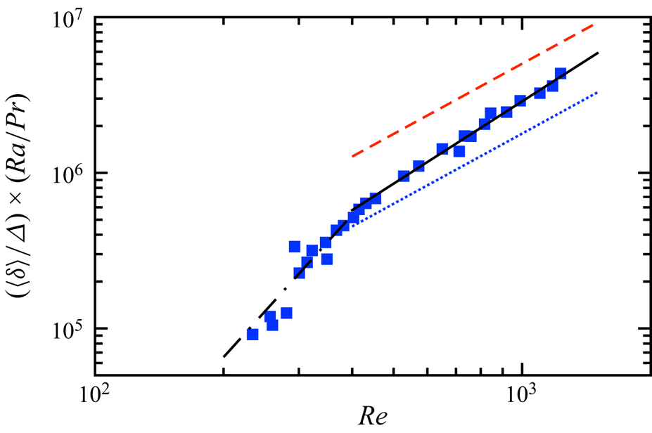
Figure 16. The measured value of  $\langle \delta \rangle /\varDelta \times Ra/Pr$ as a function of
  $Re$. Here,
  $Re_{f_0}$ is based on the peak frequency of the temperature spectra. Measurements are taken at
  $\xi =0.063, z/L=0.51$ in convection cell B. The dotted-dashed line is a power-law fit
  $\langle \delta \rangle /\varDelta \times Ra/Pr=0.007Re^{3.0\pm 0.6}$ to the data
  $Re<4.5\times 10^{3}$. The solid line is the fit of
  $\langle \delta \rangle /\varDelta \times Ra/Pr=15.4Re^{1.76\pm 0.06}$ to the data
  $Re>4.5\times 10^{3}$. The dashed line is the fit of
  $18{\rm \pi} Re^{3/2}$, the theoretical prediction from Brown & Ahlers (Reference Brown and Ahlers2008b). The dotted line is the fit of
  $159Re^{3/2}$ to the experimental data from figure 9 of Brown & Ahlers (Reference Brown and Ahlers2008b) for
  $Pr=3.3$,
  $4.4$ and
  $5.5$.

Figure 17. The experimental data of the LSC flow strength against  $Ra$. Open squares, this work from cell A; solid squares, this work from cell B; inverted triangles, data from Brown & Ahlers (Reference Brown and Ahlers2007); triangles, data from Wei & Ahlers (Reference Wei and Ahlers2016); circles, data from He et al. (Reference He, Bodenschatz and Ahlers2016). The dotted line is
  $\langle \delta \rangle /\varDelta =0.0047$, which is the value in conduction regime. The dashed line is
  $\langle \delta \rangle /\varDelta = 0.20-0.0083\log {Ra}$; The solid line is
  $\langle \delta \rangle /\varDelta = 0.068-0.0024\log {Ra}$.
In the present work, the oscillation regime can be identified only for  $Ra=1.35\times 10^5$ and
  $1.65\times 10^5$. It is difficult to see the oscillation regime from the time trace of any temperature measurement in the wall, but this regime can be found from the power spectra of the temperature measured in the sidewall in figure 14(a), an obvious peak at the oscillation frequency
  $f_0$ can be identified. Here, the values of
  $f_0$ were found to be
  $0.061$ and
  $0.038$ Hz for
  $Ra=1.46\times 10^5$ with
  $\varDelta =10.00$ K and
  $1.65\times 10^5$ with
  $\varDelta =4.00$ K. To compare our oscillation frequency with the oscillation frequency of the LSC corresponding to the LSC turnover frequency in the turbulence regime, we employed the dimensionless
  $Re$ based on the oscillation frequency in (3.3). Values of
  $Re=41.08$ and
  $43.91$ were obtained for
  $Ra=1.46\times 10^5$ with
  $\varDelta =10.00$ K and
  $1.65\times 10^5$ with
  $\varDelta =4.00$ K. The compensated quantities
  $ReRa^{-1/2}$ are
  $0.1075$ and
  $0.1081$. We plot
  $ReRa^{-1/2}Pr^{0.62}$ for these two
  $Ra$ values as a dashed line in figure 15(b). Surprisingly, the results are consistent with those for larger
  $Pr$.
$Pr$.
4. Discussion
Our results suggest that LSC is an analogy to low  $Ra$ structures. The trend of the LSC flow strength as
  $Ra$ varies under turbulence is similar to the trend of the cellular pattern in the convection and chaotic regimes. One might expect that the LSC strength at larger
  $Ra$ (far beyond hard turbulence) shows a decrease with increasing
  $Ra$ similar to that in the transition regime. Therefore, we plot our data and the LSC strength of Brown & Ahlers (Reference Brown and Ahlers2007) with
  $Pr=4.38$ and
  $3\times 10^{9}< Ra<2\times 10^{10}$ in figure 17. The LSC strength with
  $Pr=12.3$ and
  $6\times 10^{10}< Ra<6\times 10^{11}$ of Wei & Ahlers (Reference Wei and Ahlers2016) and the
  $\langle \delta \rangle /\varDelta$ with
  $Pr\sim 0.7$ and
  $10^{12}< Ra<2\times 10^{14}$ of He, Bodenschatz & Ahlers (Reference He, Bodenschatz and Ahlers2016) are also plotted for comparison. In Brown & Ahlers (Reference Brown and Ahlers2007), the data were fitted by the power law
  $21Ra^{-0.32}$. Here, we plot the data on a semi-logarithmic scale because the difference in
  $\langle \delta \rangle /\varDelta$ can be illustrated better this way. Clearly, the trend of the flow strength as
  $Ra$ varies at large
  $Ra$ in the hard turbulence regime is similar to the trends in the chaotic and transition regimes. The transition between the two lines in figure 17 is
  $4\times 10^{9}$, which is close to the value reported in Brown & Ahlers (Reference Brown and Ahlers2007), beyond which the twisting motion and the
  $Re$ value based on the turnover time show discrepancies. For
  $Ra\leqslant 3\times 10^{9}$, the experimental results of Brown & Ahlers (Reference Brown and Ahlers2007) and Xi, Zhou & Xia (Reference Xi, Zhou and Xia2006) suggest the existence of a new LSC state in which the plumes and the LSC are no longer slaved to each other and where the twist oscillation of the LSC is no longer synchronous with the LSC turnover time. For
  $Ra>3\times 10^{11}$, the data with
  $Pr=12.3$ in figure 17 show another transition, but confirming this phenomenon requires more measurements at larger
  $Ra$ and
  $Pr>1$. When
  $Ra$ is further increased, the data of He et al. (Reference He, Bodenschatz and Ahlers2016) show that a statistically well defined, albeit highly fluctuating single-roll LSC still exists in both the classic regime
  $Ra<2\times 10^{13}$ and the ultimate regime
  $Ra>2\times 10^{13}$. It is noted that at such large
  $Ra$, those authors found
  $E_1/E_{tot}\sim 0.5$, which is similar to the transition regime. Therefore, it will be interesting to see whether a stronger single-roll structure forms in the RBC with
  $\varGamma =1$ and
  $Ra$ larger than that in He et al. (Reference He, Bodenschatz and Ahlers2016).
Another interesting result of the present work is the different responses of the LSC flow strength to the turbulent background in the soft turbulence and hard turbulence regimes. In this context it would be helpful to be able to quantify the turbulent background in some way. However, the temperature measurement in the sidewall does not show any reasonable sign indicating a stronger turbulent background at larger  $Ra$. According to the previous literature, a turbulent background in RBC results in a Gaussian-like temperature distribution at the cell centre whose tails show an exponential trend caused by the thermal plume. Numerous studies have shown that in the soft and hard turbulence regimes, the temperature distribution in the cell centre evolves from a Gaussian function to a stretched exponential function, which reveals that the turbulent background is stronger at larger
  $Ra$. Numerous quantities have been proposed to quantify the strength of turbulent backgrounds. Recently, the analytical expression proposed by Wang et al. (Reference Wang, He and Tong2019) provided a straightforward quantity, the ratio of the thermal plume strength to the turbulent background strength. However, the plume strength in the cell centre is beyond the scope of the present work, the main measurements of which were taken from the sidewall, and thus, we will not discuss this phenomenon any further here.
5. Summary
In summary, we performed experiments for two  $\varGamma =1$ cylindrical RBC cells with nitrogen gas as the working fluid and measured the flow strength in the horizontal mid-height plane. The
  $Ra$ range on which we focused extended from
  $Ra=1\times 10^3$ to
  $Ra=1 \times 10^{9}$. From the flow strength, seven regimes were identified: conduction, convection, oscillation, chaotic, transition, soft turbulence and hard turbulence. In the convection regime, the flow forms a pattern corresponding to a single roll. In the oscillation regime, an oscillation frequency showing a peak in the temperature power spectra in the sidewall can be identified. In the chaotic regime, the flow is time-dependent, and the time-averaged flow strength decreases as
  $Ra$ increases. In the transition regime, the time-averaged flow strength also decreases with increasing
  $Ra$. Under soft turbulence, the LSC self-organises, and the flow strength increases with increasing
  $Ra$, whereas under hard turbulence, the LSC flow strength decreases as
  $Ra$ increases. The time-averaged flow strengths in the soft turbulence and hard turbulence regimes are similar to those in the convection and chaotic regimes, suggesting that LSC is an analogy to the cellular pattern at large
  $Ra$. This finding also indicates that at the larger
  $Ra$ of hard turbulence, the LSC will persist and show another sudden change with increasing
  $Ra$, similar to the transition regime. However, the difference remains between cellular pattern and LSC, that their preferred orientations are different. In addition, a comparison with other experimental data at larger
  $Ra$ was made, and the
  $Re$ based on the LSC turnover time was measured. We found that two power laws,
  $\langle \delta \rangle /\varDelta \times Ra/Pr = 0.007Re^{3.0}$ and
  $\langle \delta \rangle /\varDelta \times Ra/Pr = 15.4Re^{1.76}$, fit our data for
  $Re<400$ and for
  $Re>400$, respectively. The result lies between the predicted values and the measured values for
  $Pr>3$ in water.
Although the present experiment has provided a fairly detailed overall picture of the pattern close to onset of convection and the LSC at high Ra in this system, there remain some unresolved issues. One of them is the dependence of transitions between various regimes on the wall admittance. A more detailed experimental investigation with the other wall admittance should be carried out. Another feature that might be studied in more detail is the Reynolds number based on LSC oscillation frequency in other Pr and larger Ra. The present results of Re are inconsistent with either predicted values or previous measurement in water, and both the Pr and Ra are smaller than in previous work. Of course, as the range of Pr and Ra expands, the richness of phenomena seems without limit.
Acknowledgements
The experiment was conducted in Guenter Ahler's lab at the University of California, Santa Barbara. P.W. is very grateful to G. Ahlers for his guidance.
Funding
The author wishes to acknowledge financial support from the National Natural Science Foundation of China (grant no. 11702196).
Declaration of interests
The author reports no conflict of interest.
Appendix A. Critical Rayleigh numbers  $Ra_c$ and $Ra_s$


Numerous studies have reported a linear increase in the cellular pattern strength as  $Ra$ increases at the onset of convection. However, owing to the limit on the number of data points in our work, a logarithmic function was used to determine
  $Ra_c$. To show that fitting the data by a logarithmic function, and fitting them by a function as
  $k(Ra-Ra_c)^{1/2}$ yield the same result, as in figure 18(a), we plot the fits by a logarithmic function and a linear function. The results are in agreement. The same analysis was performed to determine
  $Ra_s$, the onset of soft turbulence, as shown in figure 18(b). The
  $Ra_s$ values obtained by the two functions give almost the same result.
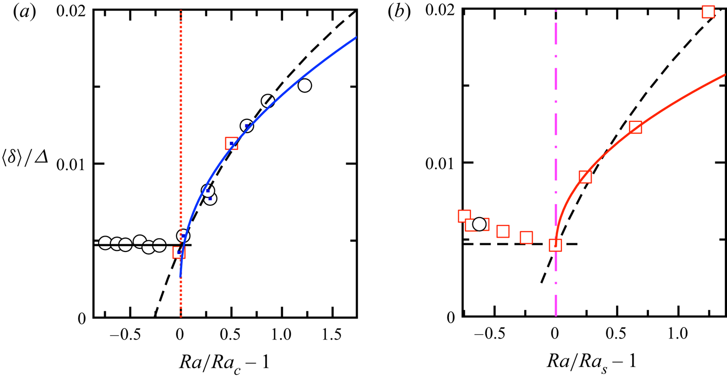
Figure 18. (a) The experimental data of the strength of the cellular pattern against  $Ra/Ra_c-1$. Here,
  $Ra_c=7300$ was fitted from a logarithmic function for the data
  $Ra_c\leqslant Ra\leqslant 2Ra_c$, shown as dashed lines. The vertical line represents
  $Ra_c$. (b) The experimental data of the LSC flow strength against
  $Ra/Ra_s-1$. Here, the onset of soft turbulence
  $Ra_s=8.38\times 10^6$ was fitted from a logarithmic function for the data
  $Ra_s\leqslant Ra \leqslant 2.5Ra_s$, shown by the dashed line. In (a,b), the dotted line is the value of
  $0.0047$ measured in the conduction regime, which is also considered as the measurement error. The solid lines are fitted by equation
  ${\langle \delta \rangle /\varDelta =k(Ra/\eta -1)^{1/2}}$, here
  $k=0.012$,
  $\eta =Ra_C$ for (a) and
  $k=0.010$,
  $\eta =Ra_S$ for (b).
Appendix B. Numerical values of the data shown in figure 10(a)
Tables 2 and 3 list the time-averaged strength  $\langle \delta \rangle /\varDelta$ as a function of
  $Ra$ plotted in figure 10(a).
Table 2. Time-averaged strength  $\langle \delta \rangle /\varDelta$ as a function of
  $Ra$. Cell A,
  $\varDelta =4.00$ K and
  $Pr=0.72$ (circles, figure 10a).
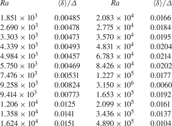
Table 3. Time-averaged strength  $\langle \delta \rangle /\varDelta$ as a function of
  $Ra$. Cell A,
  $\varDelta =10.00$ K and
  $Pr=0.72$ (circles, figure 10a).