


1 Introduction
The rotating-disk boundary-layer flow is of interest with relation to the cross-flow instability and the subsequent breakdown to turbulence. This flow is also called the von Kármán rotating-disk flow since a similarity solution for the laminar boundary layer was found by von Kármán (Reference von Kármán1921). The solution consists of an azimuthal velocity component which is dragged along with the disk, a radial velocity directed outwards with an inflectional profile normal to the disk and a vertical velocity component directed towards the disk surface. The radial inflectional component makes the flow susceptible to an inviscid cross-flow instability manifesting itself as stationary inclined vortices around the disk in experiments (Kobayashi, Kohama & Takamadate Reference Kobayashi, Kohama and Takamadate1980). These stationary vortices are triggered by the ‘rough’ disk surface – where ‘rough’ can be as small as micrometres (
 $\unicode[STIX]{x03BC}$
m) for a disk with a diameter of a metre. Commonly 28 to 32 vortices are observed in the circumferential direction, and they can be accurately described by local linear theory (Appelquist et al.
Reference Appelquist, Imayama, Alfredsson, Schlatter and Lingwood2016a
).
$\unicode[STIX]{x03BC}$
m) for a disk with a diameter of a metre. Commonly 28 to 32 vortices are observed in the circumferential direction, and they can be accurately described by local linear theory (Appelquist et al.
Reference Appelquist, Imayama, Alfredsson, Schlatter and Lingwood2016a
).
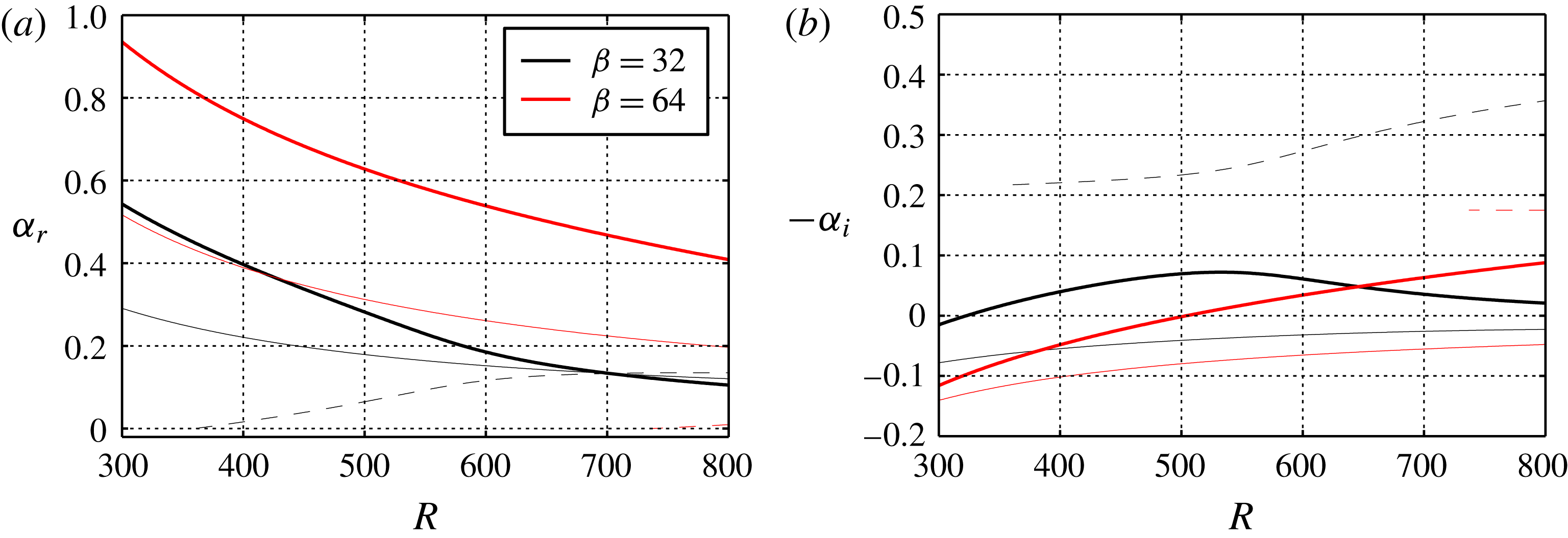
Figure 1. Stationary modes (with respect to the disk surface) for
 $\unicode[STIX]{x1D6FD}=32$
and
$\unicode[STIX]{x1D6FD}=32$
and
 $\unicode[STIX]{x1D6FD}=64$
. Keys: Type-I (——), Type-II (——), and Type-III (- - -). Only the Type-I mode is growing since
$\unicode[STIX]{x1D6FD}=64$
. Keys: Type-I (——), Type-II (——), and Type-III (- - -). Only the Type-I mode is growing since
 $-\unicode[STIX]{x1D6FC}_{i}<0$
for Type-II, and
$-\unicode[STIX]{x1D6FC}_{i}<0$
for Type-II, and
 $-\unicode[STIX]{x1D6FC}_{i}>0$
for the upstream Type-III mode. When
$-\unicode[STIX]{x1D6FC}_{i}>0$
for the upstream Type-III mode. When
 $\unicode[STIX]{x1D6FD}$
is doubled from 32 to 64 it can be seen in (a) that
$\unicode[STIX]{x1D6FD}$
is doubled from 32 to 64 it can be seen in (a) that
 $\unicode[STIX]{x1D6FC}_{r}$
is larger.
$\unicode[STIX]{x1D6FC}_{r}$
is larger.
Since 1921, when von Kármán published his paper on the similarity solution, this flow has been studied as a prototype for three-dimensional boundary layers. The rotating disk is more complex than two-dimensional boundary layers but simpler than other three-dimensional flows due to the similarity solution. It also lacks additional parameters such as a sweep angle. Research on the rotating-disk flow is fundamental to improving our overall knowledge of instabilities and Lingwood & Alfredsson (Reference Lingwood and Alfredsson2015) follow almost 100 years of research with regards to this flow. The disk configuration can also be found in technical applications and the research has additional relevance for chemical vapour deposition (CVD) (Hussain, Garrett & Stephen Reference Hussain, Garrett and Stephen2011) and computer storage devices (Oh et al. Reference Oh, Kim, Jo, Kim, Choi, Moon and Chung2012). Also, rotating disks are part of the rotor-stator flows (Serre, Tuliszka-Sznitko & Bontoux Reference Serre, Tuliszka-Sznitko and Bontoux2004) that are typically found between rotating compressors and turbine disks.
The cross-flow instability is also called the Type-I instability and is the strongest growing type of instability, although there are also Type-II and III modes. The Type-II mode is a viscous mode, which is also unstable, and the Type-III mode is a damped upstream-travelling mode. Figure 1 shows (a) the radial wavenumbers and (b) the radial growth rates of the Type-I, II and III stationary modes as function of Reynolds number for the azimuthal wavenumbers
 $\unicode[STIX]{x1D6FD}=32$
and
$\unicode[STIX]{x1D6FD}=32$
and
 $64$
. The Reynolds number is defined to be equal to the non-dimensional radius
$64$
. The Reynolds number is defined to be equal to the non-dimensional radius
 $$\begin{eqnarray}\displaystyle R=r^{\ast }\sqrt{\frac{\unicode[STIX]{x1D6FA}^{\ast }}{\unicode[STIX]{x1D708}}}=r, & & \displaystyle\end{eqnarray}$$
where
 $^{\ast }$
refers to a dimensional quantity,
$^{\ast }$
refers to a dimensional quantity,
 $r^{\ast }$
is the radial position on the disk and
$r^{\ast }$
is the radial position on the disk and
 $\unicode[STIX]{x1D6FF}^{\ast }=\sqrt{\unicode[STIX]{x1D708}/\unicode[STIX]{x1D6FA}^{\ast }}$
is the length scale used, where
$\unicode[STIX]{x1D6FF}^{\ast }=\sqrt{\unicode[STIX]{x1D708}/\unicode[STIX]{x1D6FA}^{\ast }}$
is the length scale used, where
 $\unicode[STIX]{x1D708}$
is the (dimensional) kinematic viscosity of the fluid and
$\unicode[STIX]{x1D708}$
is the (dimensional) kinematic viscosity of the fluid and
 $\unicode[STIX]{x1D6FA}^{\ast }$
is the angular velocity of the disk. The azimuthal wavenumber (
$\unicode[STIX]{x1D6FA}^{\ast }$
is the angular velocity of the disk. The azimuthal wavenumber (
 $\unicode[STIX]{x1D6FD}$
) is normalized such that it gives the number of waves over one disk circumference whereas the radial wavenumber (
$\unicode[STIX]{x1D6FD}$
) is normalized such that it gives the number of waves over one disk circumference whereas the radial wavenumber (
 $\unicode[STIX]{x1D6FC}$
) is made non-dimensional with
$\unicode[STIX]{x1D6FC}$
) is made non-dimensional with
 $\unicode[STIX]{x1D6FF}^{\ast }$
. It is clear from figure 1(b) that the strongest growing stationary mode is the Type-I mode for both wavenumbers.
$\unicode[STIX]{x1D6FF}^{\ast }$
. It is clear from figure 1(b) that the strongest growing stationary mode is the Type-I mode for both wavenumbers.
Moving towards higher Reynolds numbers, the experimentally observed (Type-I) 28 to 32 primary stationary vortices deviate from linear theory and saturate at a finite amplitude. For
 $R\gtrsim 500$
Kobayashi et al. (Reference Kobayashi, Kohama and Takamadate1980) obtained a striped pattern on top of these vortices in their flow visualizations, assumed to be secondary instabilities (their figure 8). Four to five wedges in the azimuthal direction including vortices with stripes were seen to become turbulent and form a distinct circle, see their figure 7. This transition region, differing from the jagged pattern on swept wings which also have the cross-flow instability (Saric, Carrillo & Reibert Reference Saric, Carrillo and Reibert1998), was hypothesized to be due to an absolute instability by Lingwood (Reference Lingwood1995), and that was also found theoretically by her. The absolute instability has been further investigated in direct numerical simulations (DNS). Davies & Carpenter (Reference Davies and Carpenter2003) found that the local absolute instability does not give rise to a globally unstable flow in their unconfined domain. However, when turbulence is involved, Appelquist et al. (Reference Appelquist, Schlatter, Alfredsson and Lingwood2016b
) have shown that the mean flow modified by turbulence acts as a confinement and a global instability appears where the turbulence triggers the global frequency. The critical Reynolds number for the local absolute instability is
$R\gtrsim 500$
Kobayashi et al. (Reference Kobayashi, Kohama and Takamadate1980) obtained a striped pattern on top of these vortices in their flow visualizations, assumed to be secondary instabilities (their figure 8). Four to five wedges in the azimuthal direction including vortices with stripes were seen to become turbulent and form a distinct circle, see their figure 7. This transition region, differing from the jagged pattern on swept wings which also have the cross-flow instability (Saric, Carrillo & Reibert Reference Saric, Carrillo and Reibert1998), was hypothesized to be due to an absolute instability by Lingwood (Reference Lingwood1995), and that was also found theoretically by her. The absolute instability has been further investigated in direct numerical simulations (DNS). Davies & Carpenter (Reference Davies and Carpenter2003) found that the local absolute instability does not give rise to a globally unstable flow in their unconfined domain. However, when turbulence is involved, Appelquist et al. (Reference Appelquist, Schlatter, Alfredsson and Lingwood2016b
) have shown that the mean flow modified by turbulence acts as a confinement and a global instability appears where the turbulence triggers the global frequency. The critical Reynolds number for the local absolute instability is
 $R_{c}=507$
whereas the critical Reynolds number for the global instability for the same wavenumber
$R_{c}=507$
whereas the critical Reynolds number for the global instability for the same wavenumber
 $\unicode[STIX]{x1D6FD}=68$
is
$\unicode[STIX]{x1D6FD}=68$
is
 $R_{cg}=583$
.
$R_{cg}=583$
.
For the global transition scenario described above, stationary vortices were not present; only an impulse response was investigated. The lack of stationary vortices in those simulations is inconsistent with experimental observations, where the onset of nonlinearity is found to be at
 $R=510{-}520$
(Imayama, Alfredsson & Lingwood Reference Imayama, Alfredsson and Lingwood2013), suggesting that other disturbances, mainly the stationary vortices present in all experiments, modify the flow such that transition is at smaller radii. Within this paper the focus is, therefore, on the convective instability of the stationary vortices and the transition of the modified flow. The stationary convective instability arises due to a modelled roughness element within the DNS and the main investigation reported here deals with varying the amplitude of this roughness. Further research with regard to the global instability has continued, e.g. the effects of either suction and injection (Thomas & Davies Reference Thomas and Davies2010; Ho, Corke & Matlis Reference Ho, Corke and Matlis2016), or by incorporating an axial magnetic field (Thomas & Davies Reference Thomas and Davies2013).
$R=510{-}520$
(Imayama, Alfredsson & Lingwood Reference Imayama, Alfredsson and Lingwood2013), suggesting that other disturbances, mainly the stationary vortices present in all experiments, modify the flow such that transition is at smaller radii. Within this paper the focus is, therefore, on the convective instability of the stationary vortices and the transition of the modified flow. The stationary convective instability arises due to a modelled roughness element within the DNS and the main investigation reported here deals with varying the amplitude of this roughness. Further research with regard to the global instability has continued, e.g. the effects of either suction and injection (Thomas & Davies Reference Thomas and Davies2010; Ho, Corke & Matlis Reference Ho, Corke and Matlis2016), or by incorporating an axial magnetic field (Thomas & Davies Reference Thomas and Davies2013).
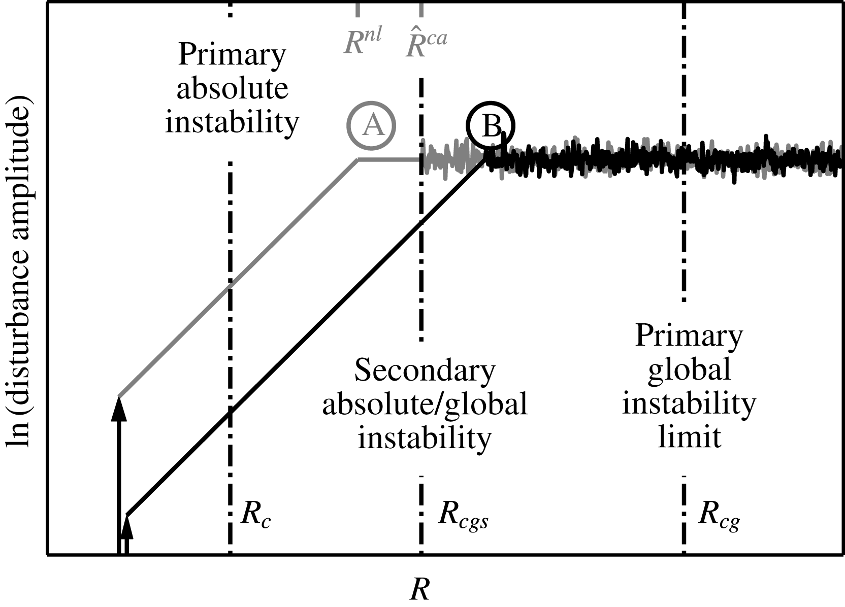
Figure 2. An illustration of the flow behaviour according to the theory of Pier (Reference Pier2007). Two different amplitude disturbances consisting of the same temporal frequency and azimuthal wavenumber are shown to grow linearly at first until they saturate or reach the same level of amplitude, followed by a disordered (turbulent) state. Ⓐ shows the content of Pier’s (Reference Pier2007) figure 3(b) where also
 $R^{nl}$
and
$R^{nl}$
and
 $\hat{R}^{ca}$
are given.
$\hat{R}^{ca}$
are given.
In addition to the primary stationary vortices, secondary instabilities can develop on top of these and have been theoretically studied by Balachandar, Streett & Malik (Reference Balachandar, Streett and Malik1992) and Pier (Reference Pier2003, Reference Pier2007). Balachandar et al. (Reference Balachandar, Streett and Malik1992) found that the primary vortex amplitude should be larger than 9 % of the mean flow for the secondary convective disturbances to grow significantly, and an increased amplitude of the primary vortex gives a higher growth rate. There is also an effect of the Reynolds number, i.e. the growth rate of the secondary instability increases with the Reynolds number. Pier (Reference Pier2003, Reference Pier2007) clarified the theoretical scenario for the rotating-disk boundary layer by including both primary and secondary stability analyses. If in this scenario there are no external perturbations, the absolute instability will set in at
 $R_{c}=507$
due to the local nature of his primary stability analysis. Pier (Reference Pier2003) studied the naturally selected outward-spiralling nonlinear vortices created by the continuous perturbation of the absolute instability. These are in turn absolutely unstable to secondary instabilities, and it is shown that the rotating-disk boundary layer can be analysed in terms of an ‘elephant’ global mode, similar to the rotating cavity described by Viaud, Serre & Chomaz (Reference Viaud, Serre and Chomaz2008, Reference Viaud, Serre and Chomaz2011). In addition, Yim et al. (Reference Yim, Chomaz, Marinand and Serre2017) observed that the growth rate of fluctuations in the rotating cavity could decrease and show smoother fronts when a superposition of spanwise wavenumbers is considered, however, leaving the underlying transition scenario unaffected. Furthermore, in the work of Pier (Reference Pier2007), harmonic forcing is applied at a frequency that does not excite the primary absolute instability. In this case, primary nonlinear waves are generated leading similarly to a secondary absolute instability and to transition, if the frequency and azimuthal wavenumber of the forcing are chosen properly. This is of interest here since the local absolute instability does not translate to an unstable global flow at exactly
$R_{c}=507$
due to the local nature of his primary stability analysis. Pier (Reference Pier2003) studied the naturally selected outward-spiralling nonlinear vortices created by the continuous perturbation of the absolute instability. These are in turn absolutely unstable to secondary instabilities, and it is shown that the rotating-disk boundary layer can be analysed in terms of an ‘elephant’ global mode, similar to the rotating cavity described by Viaud, Serre & Chomaz (Reference Viaud, Serre and Chomaz2008, Reference Viaud, Serre and Chomaz2011). In addition, Yim et al. (Reference Yim, Chomaz, Marinand and Serre2017) observed that the growth rate of fluctuations in the rotating cavity could decrease and show smoother fronts when a superposition of spanwise wavenumbers is considered, however, leaving the underlying transition scenario unaffected. Furthermore, in the work of Pier (Reference Pier2007), harmonic forcing is applied at a frequency that does not excite the primary absolute instability. In this case, primary nonlinear waves are generated leading similarly to a secondary absolute instability and to transition, if the frequency and azimuthal wavenumber of the forcing are chosen properly. This is of interest here since the local absolute instability does not translate to an unstable global flow at exactly
 $R_{c}=507$
(Davies, Thomas & Carpenter Reference Davies, Thomas and Carpenter2007; Appelquist et al.
Reference Appelquist, Schlatter, Alfredsson and Lingwood2016b
). A harmonic forcing followed by primary nonlinear waves carrying a secondary absolute instability could, however, explain the earlier transition point seen in experiments compared to
$R_{c}=507$
(Davies, Thomas & Carpenter Reference Davies, Thomas and Carpenter2007; Appelquist et al.
Reference Appelquist, Schlatter, Alfredsson and Lingwood2016b
). A harmonic forcing followed by primary nonlinear waves carrying a secondary absolute instability could, however, explain the earlier transition point seen in experiments compared to
 $R_{cg}$
. The most interesting harmonic forcing is for zero frequency, i.e. the forcing generated by stationary roughnesses on the disk surface, which are unavoidable to greater or lesser extent in experiments, and this is studied here.
$R_{cg}$
. The most interesting harmonic forcing is for zero frequency, i.e. the forcing generated by stationary roughnesses on the disk surface, which are unavoidable to greater or lesser extent in experiments, and this is studied here.
According to the theory of Pier (Reference Pier2007), there are two positions playing a role in the flow field, the saturation location beyond which finite-amplitude cross-flow vortices develop (Pier’s
 $R^{nl}$
), and the onset of the secondary absolute instability (Pier’s
$R^{nl}$
), and the onset of the secondary absolute instability (Pier’s
 $\hat{R}^{ca}$
). Figure 2 is used to illustrate this, where two different amplitude disturbances consisting of the same temporal frequency and azimuthal wavenumber are shown. The illustration includes the content of figure 3(b) in the work by Pier (Reference Pier2007) where the high-amplitude case is shown, Ⓐ. Also the primary global instability limit,
$\hat{R}^{ca}$
). Figure 2 is used to illustrate this, where two different amplitude disturbances consisting of the same temporal frequency and azimuthal wavenumber are shown. The illustration includes the content of figure 3(b) in the work by Pier (Reference Pier2007) where the high-amplitude case is shown, Ⓐ. Also the primary global instability limit,
 $R_{cg}$
, is included. Both disturbances grow exponentially at first and then saturate, here illustrated by reaching a certain amplitude level. If the saturation location is at lower
$R_{cg}$
, is included. Both disturbances grow exponentially at first and then saturate, here illustrated by reaching a certain amplitude level. If the saturation location is at lower
 $R$
than the onset of secondary absolute instability (Ⓐ high-amplitude forcing), the flow will reach a disordered state at the onset location. If the saturation location is at higher
$R$
than the onset of secondary absolute instability (Ⓐ high-amplitude forcing), the flow will reach a disordered state at the onset location. If the saturation location is at higher
 $R$
than the onset (Ⓑ low-amplitude forcing), the flow will reach a disordered state immediately on saturation. The forcing amplitude thus determines the transition scenario. Both these scenarios undergo transition at lower
$R$
than the onset (Ⓑ low-amplitude forcing), the flow will reach a disordered state immediately on saturation. The forcing amplitude thus determines the transition scenario. Both these scenarios undergo transition at lower
 $R$
than the primary global instability limit. The onset of secondary absolute instability (
$R$
than the primary global instability limit. The onset of secondary absolute instability (
 $\hat{R}^{ca}$
) is dependent on the frequency and azimuthal wavenumber of the forcing (Pier Reference Pier2007), and for our DNS only stationary vortices are considered with a wavenumber
$\hat{R}^{ca}$
) is dependent on the frequency and azimuthal wavenumber of the forcing (Pier Reference Pier2007), and for our DNS only stationary vortices are considered with a wavenumber
 $\unicode[STIX]{x1D6FD}=32$
. We will report further on these scenarios in this paper including a secondary global instability limit (
$\unicode[STIX]{x1D6FD}=32$
. We will report further on these scenarios in this paper including a secondary global instability limit (
 $R_{cgs}$
); ‘global’ due to the framework of our simulations.
$R_{cgs}$
); ‘global’ due to the framework of our simulations.
 $R_{cgs}$
is the global correspondence of
$R_{cgs}$
is the global correspondence of
 $\hat{R}^{ca}$
from local theory and can also be seen in figure 2. Note that figure 2 does not account for any possible secondary convective instability.
$\hat{R}^{ca}$
from local theory and can also be seen in figure 2. Note that figure 2 does not account for any possible secondary convective instability.
A cross-flow instability also generates streamwise vortices on a swept wing. Depending on the initial disturbance that triggers a cross-flow mode, the vortices can be either stationary or travelling with respect to the wall, which is also the case for the rotating disk. The stationary kind is seen where roughnesses on the surface give rise to the stationary vortices and the travelling kind is common in a high disturbance environment. Extensive research has been done on the cross-flow vortices on swept wings, and for instance Wassermann & Kloker (Reference Wassermann and Kloker2002, Reference Wassermann and Kloker2003) investigate both the stationary and travelling vortices. For the stationary vortices they performed DNS both in order to look at the downstream growth into a nonlinear saturated state, and to investigate the additionally triggered secondary instability. In the latter case with a triggered background condition, the steady nonlinear disturbance state experiences a sudden breakdown of the dominating nonlinear cross-flow vortices. In the transition region they found temporal frequencies of 20 and 160 to be particularly amplified (non-dimensionalized by
 $\bar{U}_{\infty }=30~\text{ms}^{-1}$
and
$\bar{U}_{\infty }=30~\text{ms}^{-1}$
and
 $\bar{L}=0.05$
m using their notation). When investigating the conditions for transition onset, the low turbulence background condition was turned off, and the flow returned to the initial nonlinear saturated state. The secondary instability causing the breakdown in the flow over their wing thus indicates a convective nature.
$\bar{L}=0.05$
m using their notation). When investigating the conditions for transition onset, the low turbulence background condition was turned off, and the flow returned to the initial nonlinear saturated state. The secondary instability causing the breakdown in the flow over their wing thus indicates a convective nature.
Brynjell-Rahkola et al. (Reference Brynjell-Rahkola, Shahriari, Schlatter, Hanifi and Henningson2017) show that in the three-dimensional Falkner–Skan–Cooke boundary layer the wake of a large roughness can change into an oscillator driving a secondary instability such that the flow becomes globally unstable. They found that the first mode that becomes unstable in their simulations is the ‘z’-mode. This relates back to Malik et al. (Reference Malik, Li, Choudhari and Chang1999) who found several secondary modes when investigating secondary instabilities on the swept-wing cross-flow vortices using a quasi-parallel flow assumption. They classified the modes into ‘y’- or ‘z’-modes, where the names relate to the maximum amplitude of the modes with respect to the gradient of the mean axial velocity distribution. Malik et al. (Reference Malik, Li, Choudhari and Chang1999) found that the disturbance energy production is dominated by energy transfer associated with the gradients in either the wall-normal/
 $y$
-direction or spanwise/
$y$
-direction or spanwise/
 $z$
-direction. For the geometry of the disk these modes correspond to a ‘z’- and ‘r’-mode, respectively.
$z$
-direction. For the geometry of the disk these modes correspond to a ‘z’- and ‘r’-mode, respectively.
For the rotating-disk flow of interest here, an investigation of secondary instabilities is made both to understand the transition scenario in the presence of roughness, and to investigate their structure. For instance, Brynjell-Rahkola et al. (Reference Brynjell-Rahkola, Shahriari, Schlatter, Hanifi and Henningson2017) found that for distributed roughnesses in a cross-flow boundary layer the global eigenvalue spectrum is very sensitive to the domain size used in the simulation and the numerical parameters set for the eigenvalue solver. Appelquist et al. (Reference Appelquist, Schlatter, Alfredsson and Lingwood2015) found a similar sensitivity to the domain size where higher growth rates of the global instability were found for larger domains. However, both of these references considered a linearized framework in which the baseflow did not change. In the present case, the nonlinear governing equations are solved, which means that the influence of the edge condition, and any emerging turbulence, is allowed to propagate into the whole flow domain. This is in an effort to compare to the experimental flow case as studied by Imayama et al. (Reference Imayama, Alfredsson and Lingwood2013), such that the full route to turbulence can be analysed. Further simulations on the turbulent flow can be found in Appelquist (Reference Appelquist2017). Note that our analysis is restricted to one azimuthal wavenumber; as shown by Yim et al. (Reference Yim, Chomaz, Marinand and Serre2017) the interaction of multiple wavenumbers might reduce the growth rates.
The paper is organized as follows. In the next section (§ 2) the simulation method is described and the flow parameters for all simulations are presented. Following that, § 3 shows results where first (§ 3.1) an analysis of the critical Reynolds number for the global instability in our domain with
 $\unicode[STIX]{x1D6FD}=64$
is presented. Next (§ 3.2), the spatially fluctuating velocity is presented and discussed for all simulations, followed (§ 3.3) by results from the temporal fluctuating velocity. In § 3.4 a comparison to the swept-wing flow is presented. Finally, the conclusions are given in § 4.
$\unicode[STIX]{x1D6FD}=64$
is presented. Next (§ 3.2), the spatially fluctuating velocity is presented and discussed for all simulations, followed (§ 3.3) by results from the temporal fluctuating velocity. In § 3.4 a comparison to the swept-wing flow is presented. Finally, the conclusions are given in § 4.
2 Method
The simulations were performed with the massively parallel code Nek5000 (Fischer, Lottes & Kerkemeier Reference Fischer, Lottes and Kerkemeier2012) using a spectral-element method (SEM). The set-up is described in Appelquist et al. (Reference Appelquist, Schlatter, Alfredsson and Lingwood2015, Reference Appelquist, Schlatter, Alfredsson and Lingwood2016b ). Also here, Legendre polynomials of order 7 are used. The full Navier–Stokes equations solved within the Nek5000 code are
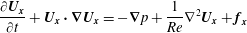 $$\begin{eqnarray}\displaystyle \frac{\unicode[STIX]{x2202}\boldsymbol{U}_{\boldsymbol{x}}}{\unicode[STIX]{x2202}t}+\boldsymbol{U}_{\boldsymbol{x}}\boldsymbol{\cdot }\unicode[STIX]{x1D735}\boldsymbol{U}_{\boldsymbol{x}}=-\unicode[STIX]{x1D735}p+\frac{1}{Re}\unicode[STIX]{x1D6FB}^{2}\boldsymbol{U}_{\boldsymbol{ x}}+\boldsymbol{f}_{\boldsymbol{x}} & & \displaystyle\end{eqnarray}$$
together with the continuity equation
 $$\begin{eqnarray}\displaystyle \unicode[STIX]{x1D735}\boldsymbol{\cdot }\boldsymbol{U}_{\boldsymbol{x}}=0, & & \displaystyle\end{eqnarray}$$
where
 $Re$
is the simulation Reynolds number,
$Re$
is the simulation Reynolds number,
 $\boldsymbol{U}_{\boldsymbol{x}}=(U_{x},U_{y},W)$
are the velocities in Cartesian coordinates,
$\boldsymbol{U}_{\boldsymbol{x}}=(U_{x},U_{y},W)$
are the velocities in Cartesian coordinates,
 $p$
is the pressure and
$p$
is the pressure and
 $\boldsymbol{f}_{\boldsymbol{x}}$
is a forcing term used in connection with the initial disturbance, fictional forces (if included) and sponge regions are used together with the radial boundary conditions. For the velocities in cylindrical coordinates the vector
$\boldsymbol{f}_{\boldsymbol{x}}$
is a forcing term used in connection with the initial disturbance, fictional forces (if included) and sponge regions are used together with the radial boundary conditions. For the velocities in cylindrical coordinates the vector
 $\boldsymbol{U}=(U,V,W)$
is used. The time scale within Nek5000 is such that
$\boldsymbol{U}=(U,V,W)$
is used. The time scale within Nek5000 is such that
 $t$
corresponds to the number of radians through which the disk has rotated. The number of full rotations is measured by
$t$
corresponds to the number of radians through which the disk has rotated. The number of full rotations is measured by
 $T=t/(2\unicode[STIX]{x03C0})$
.
$T=t/(2\unicode[STIX]{x03C0})$
.
2.1 Mesh
The domain size of the simulations conducted is shown in figure 3 in the
 $r$
–
$r$
–
 $z$
plane, and the spectral-element mesh is summarized in table 1. Only a disk angle of
$z$
plane, and the spectral-element mesh is summarized in table 1. Only a disk angle of
 $2\unicode[STIX]{x03C0}/32$
radians are simulated. In the wall-normal (
$2\unicode[STIX]{x03C0}/32$
radians are simulated. In the wall-normal (
 $z$
) direction the elements were stretched according to
$z$
) direction the elements were stretched according to
 $$\begin{eqnarray}\displaystyle z_{n}=\frac{s^{n}-1}{s-1}\unicode[STIX]{x0394}z, & & \displaystyle\end{eqnarray}$$
where
 $s$
is the stretch factor,
$s$
is the stretch factor,
 $z_{n}$
is the coordinate at position
$z_{n}$
is the coordinate at position
 $n$
above the wall (
$n$
above the wall (
 $z_{1}=\unicode[STIX]{x0394}z$
where
$z_{1}=\unicode[STIX]{x0394}z$
where
 $\unicode[STIX]{x0394}z$
is the extent of the spectral element closest to the wall). The resolution in
$\unicode[STIX]{x0394}z$
is the extent of the spectral element closest to the wall). The resolution in
 $r$
, i.e.
$r$
, i.e.
 $\unicode[STIX]{x0394}r$
, varies along the mesh. The mesh is stretched in
$\unicode[STIX]{x0394}r$
, varies along the mesh. The mesh is stretched in
 $r$
to obtain a lower resolution for
$r$
to obtain a lower resolution for
 $r<400$
and an increased resolution is applied close to
$r<400$
and an increased resolution is applied close to
 $r=700$
since this set-up includes an edge that needs to be fully resolved (see next section). The set-up is based on previous simulations of the impulse response (Appelquist et al.
Reference Appelquist, Schlatter, Alfredsson and Lingwood2016b
) and for those simulations turbulent quantities were extracted prior to creating this mesh. Here the turbulent viscous length scale
$r=700$
since this set-up includes an edge that needs to be fully resolved (see next section). The set-up is based on previous simulations of the impulse response (Appelquist et al.
Reference Appelquist, Schlatter, Alfredsson and Lingwood2016b
) and for those simulations turbulent quantities were extracted prior to creating this mesh. Here the turbulent viscous length scale
 $\ell _{\ast }$
was estimated to
$\ell _{\ast }$
was estimated to
 $3.3\times 10^{-2}$
in non-dimensional units just prior to the edge at
$3.3\times 10^{-2}$
in non-dimensional units just prior to the edge at
 $r=700$
. For a polynomial order of 7, the closest point to the wall for our mesh is at a height of
$r=700$
. For a polynomial order of 7, the closest point to the wall for our mesh is at a height of
 $z=2.6\times 10^{-2}$
corresponding to
$z=2.6\times 10^{-2}$
corresponding to
 $z^{+}=0.77$
, and for
$z^{+}=0.77$
, and for
 $z<16.6$
the resolution of the mesh is
$z<16.6$
the resolution of the mesh is
 $\unicode[STIX]{x0394}z^{+}<10$
. Appelquist et al. (Reference Appelquist, Schlatter, Alfredsson and Lingwood2016b
) also investigated meshes of different structure and polynomial resolution.
$\unicode[STIX]{x0394}z^{+}<10$
. Appelquist et al. (Reference Appelquist, Schlatter, Alfredsson and Lingwood2016b
) also investigated meshes of different structure and polynomial resolution.

Figure 3. Simulation set-up for all cases presented. ‘SYM’ denotes the symmetry boundary condition, ‘v’ the Dirichlet boundary condition, ‘O’ the homogeneous Neumann outflow and ‘ON’ a combination of ‘v’ and ‘O’, see text for further details.
Table 1. Mesh parameters including the size of the domain [min max], number of spectral elements (
 $N_{r}$
,
$N_{r}$
,
 $N_{\unicode[STIX]{x1D703}}$
and
$N_{\unicode[STIX]{x1D703}}$
and
 $N_{z}$
in the
$N_{z}$
in the
 $r$
,
$r$
,
 $\unicode[STIX]{x1D703}$
and
$\unicode[STIX]{x1D703}$
and
 $z$
directions, respectively) and resolution of the spectral elements in the radial, azimuthal and wall-normal directions. The total number of spectral elements is 388 864.
$z$
directions, respectively) and resolution of the spectral elements in the radial, azimuthal and wall-normal directions. The total number of spectral elements is 388 864.
2.2 Boundary conditions
In figure 3 a symmetry boundary condition is shown downwards of the disk edge denoted with ‘SYM’. For this condition the domain is mirrored in the
 $z$
direction corresponding to an infinitely thin disk where
$z$
direction corresponding to an infinitely thin disk where
 $W=0$
, and
$W=0$
, and
 $\unicode[STIX]{x2202}U/\unicode[STIX]{x2202}z=0$
and
$\unicode[STIX]{x2202}U/\unicode[STIX]{x2202}z=0$
and
 $\unicode[STIX]{x2202}V/\unicode[STIX]{x2202}z=0$
. Furthermore, the Dirichlet boundary condition is denoted with ‘v’ and is always set to von. A homogeneous Neumann outflow boundary condition is denoted with ‘O’, and ‘ON’ combines both v and O to set the in-plane velocities but leaves the normal velocity to be stress free. A segmentation of the domain to only
$\unicode[STIX]{x2202}V/\unicode[STIX]{x2202}z=0$
. Furthermore, the Dirichlet boundary condition is denoted with ‘v’ and is always set to von. A homogeneous Neumann outflow boundary condition is denoted with ‘O’, and ‘ON’ combines both v and O to set the in-plane velocities but leaves the normal velocity to be stress free. A segmentation of the domain to only
 $2\unicode[STIX]{x03C0}/32$
radians was done through cyclic boundary conditions in the azimuthal direction, which are essentially periodic boundary conditions but involve an appropriate rotation of the velocities across the boundary. A sponge region is used inward of the radial boundaries, it is shown as grey shaded areas in figure 3 and is described in Appelquist et al. (Reference Appelquist, Schlatter, Alfredsson and Lingwood2015). Within the sponge region, a volume force is applied to the velocity field such that the solution will go back to the von Kármán laminar flow field over the disk surface. The sponge function
$2\unicode[STIX]{x03C0}/32$
radians was done through cyclic boundary conditions in the azimuthal direction, which are essentially periodic boundary conditions but involve an appropriate rotation of the velocities across the boundary. A sponge region is used inward of the radial boundaries, it is shown as grey shaded areas in figure 3 and is described in Appelquist et al. (Reference Appelquist, Schlatter, Alfredsson and Lingwood2015). Within the sponge region, a volume force is applied to the velocity field such that the solution will go back to the von Kármán laminar flow field over the disk surface. The sponge function
 $\unicode[STIX]{x1D706}(r)$
is used in the forcing function
$\unicode[STIX]{x1D706}(r)$
is used in the forcing function
 $$\begin{eqnarray}\displaystyle \boldsymbol{f}=-\unicode[STIX]{x1D706}(r)\boldsymbol{u}, & & \displaystyle\end{eqnarray}$$
where
 $\boldsymbol{f}$
in cylindrical coordinates is converted to
$\boldsymbol{f}$
in cylindrical coordinates is converted to
 $\boldsymbol{f}_{\boldsymbol{x}}$
in Cartesian coordinates before entering (2.1) in our simulations. It is described by
$\boldsymbol{f}_{\boldsymbol{x}}$
in Cartesian coordinates before entering (2.1) in our simulations. It is described by
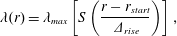 $$\begin{eqnarray}\displaystyle \unicode[STIX]{x1D706}(r)=\unicode[STIX]{x1D706}_{max}\left[S\left(\frac{r-r_{start}}{\unicode[STIX]{x1D6E5}_{rise}}\right)\right], & & \displaystyle\end{eqnarray}$$
where the maximum strength of the damping is
 $\unicode[STIX]{x1D706}_{max}$
, the radial position where the sponge region starts is
$\unicode[STIX]{x1D706}_{max}$
, the radial position where the sponge region starts is
 $r_{start}$
and
$r_{start}$
and
 $\unicode[STIX]{x1D6E5}_{rise}$
corresponds to the rise distance of the damping function. The smooth step function
$\unicode[STIX]{x1D6E5}_{rise}$
corresponds to the rise distance of the damping function. The smooth step function
 $S$
, using
$S$
, using
 $x$
as the argument, is
$x$
as the argument, is
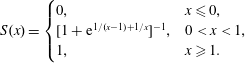 $$\begin{eqnarray}\displaystyle S(x)=\left\{\begin{array}{@{}ll@{}}0,\quad & x\leqslant 0,\\ \text{}[1+\text{e}^{1/(x-1)+1/x}]^{-1},\quad & 0<x<1,\\ 1,\quad & x\geqslant 1.\end{array}\right. & & \displaystyle\end{eqnarray}$$
The corresponding
 $\unicode[STIX]{x1D6E5}_{rise}$
parameter is seen as light grey shaded areas and the areas where
$\unicode[STIX]{x1D6E5}_{rise}$
parameter is seen as light grey shaded areas and the areas where
 $\unicode[STIX]{x1D706}_{max}$
is achieved are dark grey in figure 3. For large
$\unicode[STIX]{x1D706}_{max}$
is achieved are dark grey in figure 3. For large
 $r$
,
$r$
,
 $\unicode[STIX]{x1D706}_{max}=8$
and the sponge prior to the ‘O’ condition, only
$\unicode[STIX]{x1D706}_{max}=8$
and the sponge prior to the ‘O’ condition, only
 $V$
and
$V$
and
 $W$
were forced to zero (here there is no disk surface) to reduce the vorticity in the fields before the outflow. A sponge was also used for the inflow region where the function (2.5) was tuned to damp in the opposite direction. The inflow sponge region have
$W$
were forced to zero (here there is no disk surface) to reduce the vorticity in the fields before the outflow. A sponge was also used for the inflow region where the function (2.5) was tuned to damp in the opposite direction. The inflow sponge region have
 $\unicode[STIX]{x1D706}_{max}=0.8$
,
$\unicode[STIX]{x1D706}_{max}=0.8$
,
 $r_{start}=250$
and
$r_{start}=250$
and
 $\unicode[STIX]{x1D6E5}_{rise}=10$
used in the negative
$\unicode[STIX]{x1D6E5}_{rise}=10$
used in the negative
 $r$
-direction. The purpose of this inflow sponge region is to reduce potential spurious reflections of the upstream-travelling Type-III mode.
$r$
-direction. The purpose of this inflow sponge region is to reduce potential spurious reflections of the upstream-travelling Type-III mode.
The reason for these choices for the boundary conditions is discussed in detail in Appelquist (Reference Appelquist2014), but is summarized briefly here. The radial inflow lies in the laminar region, for which the von Kármán similarity solution is valid and is thus set as Dirichlet condition; for the radial turbulent outflow the instantaneous flow is unknown a priori, which motivates the use of a stress-free condition that does not prescribe velocity values, but only derivatives. Similarly, the Neumann conditions in the free stream are chosen to allow the boundary layer to grow based on the local flow conditions, while maintaining the (very small) radial velocity. This condition proved to be more robust than imposing a Neumann condition on the radial velocity, and does not influence the flow close to the disk (Appelquist Reference Appelquist2014).
2.3 Initial conditions and disturbances
All simulations were initialized with the von Kármán laminar boundary-layer solution. The simulations were run for 0.25 rotations to allow the flow to develop into a stable radial jet for
 $r>700$
as seen in figure 4. The influence of distributed surface roughness was modelled by a continuous volume force applied in the near-wall region of the rotating disk added at
$r>700$
as seen in figure 4. The influence of distributed surface roughness was modelled by a continuous volume force applied in the near-wall region of the rotating disk added at
 $T=0.25$
. To excite the flow continuously, a Gaussian forcing function was used as described in Appelquist et al. (Reference Appelquist, Imayama, Alfredsson, Schlatter and Lingwood2016a
) with the same parameters as their run r32. An amplitude factor defined as
$T=0.25$
. To excite the flow continuously, a Gaussian forcing function was used as described in Appelquist et al. (Reference Appelquist, Imayama, Alfredsson, Schlatter and Lingwood2016a
) with the same parameters as their run r32. An amplitude factor defined as
 $a_{f}$
is used in relation to the forcing for the simulations here where
$a_{f}$
is used in relation to the forcing for the simulations here where
 $a_{f}$
simply multiplies the forcing term
$a_{f}$
simply multiplies the forcing term
 $\boldsymbol{f}_{\boldsymbol{x}}$
that is added in relation to the roughness. Here the excitation radius is
$\boldsymbol{f}_{\boldsymbol{x}}$
that is added in relation to the roughness. Here the excitation radius is
 $r=287$
, except for the highest-amplitude case where this was moved to
$r=287$
, except for the highest-amplitude case where this was moved to
 $r=300$
. The reason for this was too much damping in the stable region for the azimuthal wavenumber
$r=300$
. The reason for this was too much damping in the stable region for the azimuthal wavenumber
 $\unicode[STIX]{x1D6FD}=32$
, which has a critical Reynolds number for Type-I stationary disturbances of
$\unicode[STIX]{x1D6FD}=32$
, which has a critical Reynolds number for Type-I stationary disturbances of
 $R=323$
(see where
$R=323$
(see where
 $-\unicode[STIX]{x1D6FC}_{i}$
becomes positive in figure 1
b).
$-\unicode[STIX]{x1D6FC}_{i}$
becomes positive in figure 1
b).
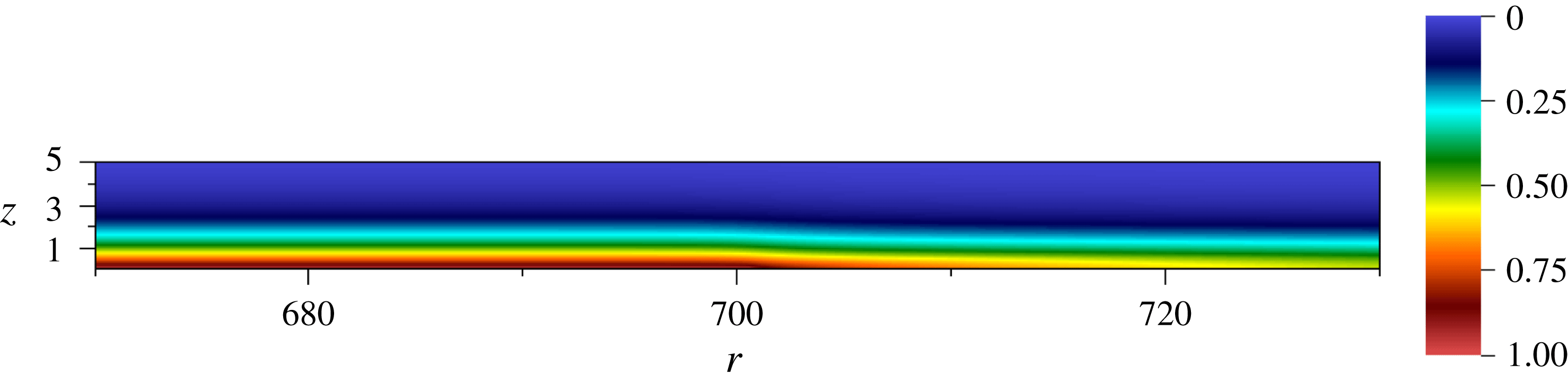
Figure 4. Azimuthal velocity normalized by the local disk velocity just before a roughness is added to the disk at
 $T=0.25$
.
$T=0.25$
.
The body force is used as a means to generate the stationary (spiral) vortices, which would emerge naturally in an experiment due to unavoidable random surface roughness. Therefore, the exact spatial shape of the forcing function is considered to be unimportant, as long as spiral vortices are generated, which initially follow linear behaviour as discussed in Appelquist et al. (Reference Appelquist, Imayama, Alfredsson, Schlatter and Lingwood2016a
). The differences relevant for the present paper start just before the deviation from the linear behaviour, i.e. for larger
 $r$
.
$r$
.
2.4 Simulations
The simulations made are summarized in table 2 together with their notation used throughout the paper. Additional simulations similar to cases A3 and A4 were also set-up with only a sponge outflow condition, i.e. no finite edge. Similar results were obtained in these cases and they are therefore not described in the paper. The main variation between the simulations is the amplitude used for the forcing,
 $a_{f}$
, denoted with ‘A1’ for the weakest amplitude through to ‘A5’ for the strongest. The highest value of
$a_{f}$
, denoted with ‘A1’ for the weakest amplitude through to ‘A5’ for the strongest. The highest value of
 $a_{f}$
was 400 since no extra effect was observed for higher amplitudes, instead the disturbance was moved to a higher radial position for case A5 (300 instead of 287) in order to achieve an elevation in amplitude further downstream, hence the notation ‘400
$a_{f}$
was 400 since no extra effect was observed for higher amplitudes, instead the disturbance was moved to a higher radial position for case A5 (300 instead of 287) in order to achieve an elevation in amplitude further downstream, hence the notation ‘400
 $+$
’.
$+$
’.
Table 2. Simulations presented in this paper together with the forcing amplitude used in each case, and comparable experimental cases for each amplitude.
The last column describes experimentally comparable cases connected to a certain forcing amplitude; the similarity will be seen from the results in § 3.2. The experimental data include two cases; case Exp
 $_{c}$
for the clean disk experiment (IP02 presented in Imayama, Alfredsson & Lingwood Reference Imayama, Alfredsson and Lingwood2014a
); and case Exp
$_{c}$
for the clean disk experiment (IP02 presented in Imayama, Alfredsson & Lingwood Reference Imayama, Alfredsson and Lingwood2014a
); and case Exp
 $_{r}$
for the rough disk experiment (EXP_rough presented in Appelquist et al.
Reference Appelquist, Imayama, Alfredsson, Schlatter and Lingwood2016a
). Exp
$_{r}$
for the rough disk experiment (EXP_rough presented in Appelquist et al.
Reference Appelquist, Imayama, Alfredsson, Schlatter and Lingwood2016a
). Exp
 $_{r}$
has 32 roughness elements equispaced azimuthally to excite 32 vortices preferentially. The
$_{r}$
has 32 roughness elements equispaced azimuthally to excite 32 vortices preferentially. The
 $v_{rms}$
data obtained at
$v_{rms}$
data obtained at
 $z=1.3$
available from these experiments were in the range
$z=1.3$
available from these experiments were in the range
 $R=360{-}700$
and
$R=360{-}700$
and
 $R=260{-}605$
, respectively.
$R=260{-}605$
, respectively.
All simulations were initially run until
 $T=2.5$
in the laboratory frame of reference. This was since the laboratory frame gives velocities after the disk edge,
$T=2.5$
in the laboratory frame of reference. This was since the laboratory frame gives velocities after the disk edge,
 $r>700$
, that decrease to zero giving a more stable simulation (larger time steps can be used). For the analysis of the secondary instability on the stationary vortices, however, the rotating reference frame is an advantage. Therefore the simulations were conducted in this frame for an additional 0.5 rotations until
$r>700$
, that decrease to zero giving a more stable simulation (larger time steps can be used). For the analysis of the secondary instability on the stationary vortices, however, the rotating reference frame is an advantage. Therefore the simulations were conducted in this frame for an additional 0.5 rotations until
 $T=3$
.
$T=3$
.
Time development data are shown in figure 5(a) in terms of
 $v_{rms}$
. These root-mean-square (r.m.s.) amplitudes are obtained as:
$v_{rms}$
. These root-mean-square (r.m.s.) amplitudes are obtained as:
 $$\begin{eqnarray}\displaystyle v_{rms}=\sqrt{\frac{1}{\unicode[STIX]{x1D6E9}}\int _{0}^{\unicode[STIX]{x1D6E9}}(V_{N}-\langle V_{N}\rangle )^{2}\,\text{d}\unicode[STIX]{x1D703}}, & & \displaystyle\end{eqnarray}$$
where
 $V_{N}$
is the azimuthal velocity normalized by the local disk velocity (
$V_{N}$
is the azimuthal velocity normalized by the local disk velocity (
 $r\unicode[STIX]{x1D6FA}$
) and the brackets define the spatial mean. For our domain
$r\unicode[STIX]{x1D6FA}$
) and the brackets define the spatial mean. For our domain
 $\unicode[STIX]{x1D6E9}=2\unicode[STIX]{x03C0}/32$
, only two runs were made for the initial 0.25 rotations where the background noise level is of the order of
$\unicode[STIX]{x1D6E9}=2\unicode[STIX]{x03C0}/32$
, only two runs were made for the initial 0.25 rotations where the background noise level is of the order of
 $10^{-14}$
for
$10^{-14}$
for
 $r=420$
and
$r=420$
and
 $z=1.3$
. In figure 5(b) the
$z=1.3$
. In figure 5(b) the
 $v_{rms}$
amplitude is shown as a function of radius and indicates the noise level of the simulations and this is seen to increase with
$v_{rms}$
amplitude is shown as a function of radius and indicates the noise level of the simulations and this is seen to increase with
 $r$
. Since the mesh resolution is higher at the edge of the disk (
$r$
. Since the mesh resolution is higher at the edge of the disk (
 $r=700$
), the only reason for this increase is the upstream-travelling disturbances from the edge when the flow downstream is adjusting from the von Kármán disk flow to a new baseflow. After
$r=700$
), the only reason for this increase is the upstream-travelling disturbances from the edge when the flow downstream is adjusting from the von Kármán disk flow to a new baseflow. After
 $T=0.25$
the disturbance was added and stationary vortices develop. On top of these there are low-amplitude secondary instabilities, which will be discussed in the result section.
$T=0.25$
the disturbance was added and stationary vortices develop. On top of these there are low-amplitude secondary instabilities, which will be discussed in the result section.
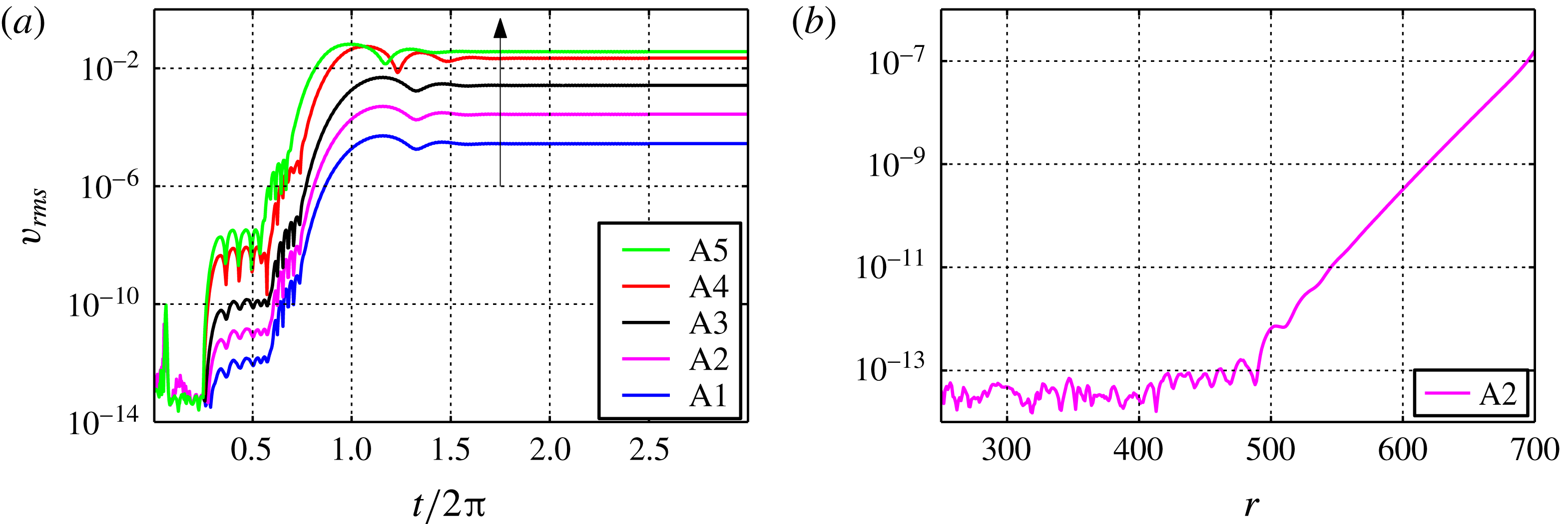
Figure 5. (a) Time development of
 $v_{rms}$
at
$v_{rms}$
at
 $r=420$
and
$r=420$
and
 $z=1.3$
. An arrow gives the direction of simulations from A1 to A5. (b) Noise level just before the disturbance was added at
$z=1.3$
. An arrow gives the direction of simulations from A1 to A5. (b) Noise level just before the disturbance was added at
 $T=0.25$
.
$T=0.25$
.
3 Results
3.1 Characteristics of the global instability
Previously Appelquist et al. (Reference Appelquist, Schlatter, Alfredsson and Lingwood2016b
) have shown that the rotating-disk boundary layer has a global instability at
 $R_{cg}=583$
for a domain simulating an azimuthal wavenumber
$R_{cg}=583$
for a domain simulating an azimuthal wavenumber
 $\unicode[STIX]{x1D6FD}=68$
. Here the simulation domain is
$\unicode[STIX]{x1D6FD}=68$
. Here the simulation domain is
 $1/32$
of the disk and while
$1/32$
of the disk and while
 $\unicode[STIX]{x1D6FD}=32$
does not give rise to a global instability, the periodicity of the domain is expected to give rise to a global instability for
$\unicode[STIX]{x1D6FD}=32$
does not give rise to a global instability, the periodicity of the domain is expected to give rise to a global instability for
 $\unicode[STIX]{x1D6FD}=64$
. Following the same procedure with an additional simulation G64, the front separating flow of small-amplitude perturbations (linear) and large-amplitude disordered perturbations (nonlinear) converges to a position of
$\unicode[STIX]{x1D6FD}=64$
. Following the same procedure with an additional simulation G64, the front separating flow of small-amplitude perturbations (linear) and large-amplitude disordered perturbations (nonlinear) converges to a position of
 $R_{cg}=599$
. This case was run for 4.5 rotations and the result is shown in its context in table 3. The global temporal frequency found in the simulation is 50.1 (
$R_{cg}=599$
. This case was run for 4.5 rotations and the result is shown in its context in table 3. The global temporal frequency found in the simulation is 50.1 (
 $-13.9$
in the rotating reference frame), and local linear theory gives
$-13.9$
in the rotating reference frame), and local linear theory gives
 $\unicode[STIX]{x1D714}_{r}=50.6$
(
$\unicode[STIX]{x1D714}_{r}=50.6$
(
 $-13.4$
) for
$-13.4$
) for
 $R_{cg}=599$
and
$R_{cg}=599$
and
 $\unicode[STIX]{x1D6FD}=64$
.
$\unicode[STIX]{x1D6FD}=64$
.

Figure 6. Instantaneous fields of
 $V_{N}$
at
$V_{N}$
at
 $z=3.6$
: (a) case A2; (b) case A5.
$z=3.6$
: (a) case A2; (b) case A5.
Table 3. Critical values for the primary absolute (
 $R_{c}$
) and primary global (
$R_{c}$
) and primary global (
 $R_{cg}$
) instability for two azimuthal wavenumbers (
$R_{cg}$
) instability for two azimuthal wavenumbers (
 $\unicode[STIX]{x1D6FD}$
).
$\unicode[STIX]{x1D6FD}$
).

Figure 7. Space–time diagrams showing
 $v_{rms}$
at
$v_{rms}$
at
 $z=1.3$
in
$z=1.3$
in
 $\log _{10}$
scale: (a) case A2; (b) case A5.
$\log _{10}$
scale: (a) case A2; (b) case A5.
3.2 Overall transition scenario
For illustrative purposes, two final instantaneous fields can be seen in figure 6(a) for case A2 and in (b) for case A5. The transition routes shown in these panels are explained later in this section by scenarios (a) Ⓑ and (b) Ⓐ (see figure 2). For small
 $r$
both simulations have stationary vortices shown as stripes in the azimuthal direction. In (a) a widening black region around
$r$
both simulations have stationary vortices shown as stripes in the azimuthal direction. In (a) a widening black region around
 $r=545$
is shown and in (b) additional stripes across the stationary vortices are shown at
$r=545$
is shown and in (b) additional stripes across the stationary vortices are shown at
 $r=500$
. For larger
$r=500$
. For larger
 $r$
both cases enter a disordered region.
$r$
both cases enter a disordered region.
In figure 7 two space–time diagrams show the development of
 $v_{rms}$
obtained at a height of
$v_{rms}$
obtained at a height of
 $z=1.3$
for the same cases (a) A2 and (b) A5. The colours are in
$z=1.3$
for the same cases (a) A2 and (b) A5. The colours are in
 $\log _{10}$
scale and it is clear that the forcing has a lower amplitude for case A2 compared to case A5. For
$\log _{10}$
scale and it is clear that the forcing has a lower amplitude for case A2 compared to case A5. For
 $T<0.25$
there is no forcing present. After the stationary forcing is introduced, both simulations have disturbances growing inwards from the edge at early times which can be traced back to the global instability, see figure 6(b) in Appelquist et al. (Reference Appelquist, Schlatter, Alfredsson and Lingwood2016b
). This global instability is triggered by low-amplitude travelling waves, which are induced by the introduction of the stationary disturbance. For later times the two simulations are different for the highest amplitudes. The amplitude increases with
$T<0.25$
there is no forcing present. After the stationary forcing is introduced, both simulations have disturbances growing inwards from the edge at early times which can be traced back to the global instability, see figure 6(b) in Appelquist et al. (Reference Appelquist, Schlatter, Alfredsson and Lingwood2016b
). This global instability is triggered by low-amplitude travelling waves, which are induced by the introduction of the stationary disturbance. For later times the two simulations are different for the highest amplitudes. The amplitude increases with
 $r$
for case A2 whereas case A5 has a clear peak around
$r$
for case A2 whereas case A5 has a clear peak around
 $R=475$
. Both simulations are seen to become turbulent without any additional tripping.
$R=475$
. Both simulations are seen to become turbulent without any additional tripping.
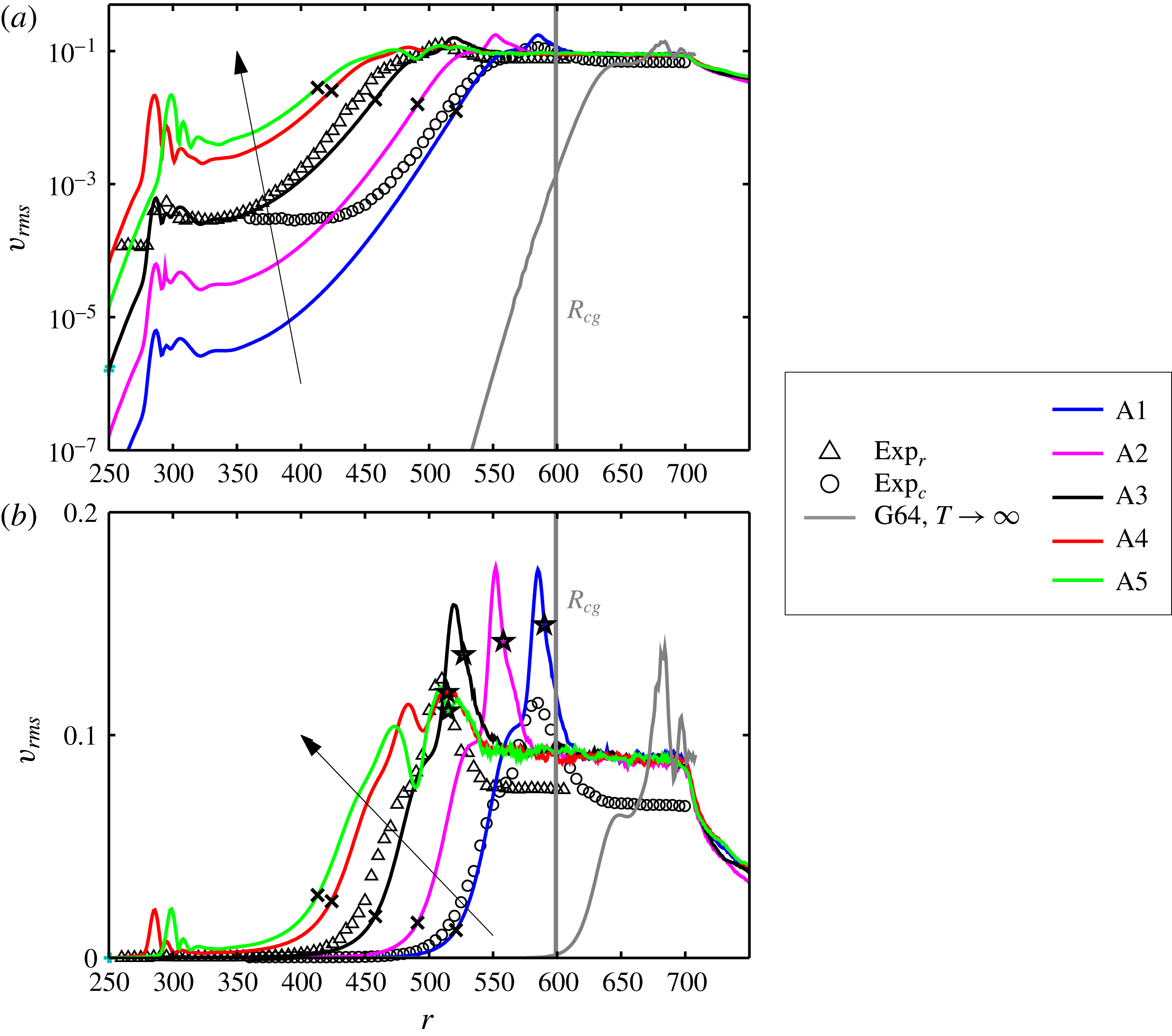
Figure 8. The azimuthal r.m.s.,
 $v_{rms}$
, as a function of
$v_{rms}$
, as a function of
 $r$
for all simulations in table 2 for
$r$
for all simulations in table 2 for
 $z=1.3$
at their final time. Arrows give the direction of simulations from A1 to A5. Additionally, the globally unstable case for
$z=1.3$
at their final time. Arrows give the direction of simulations from A1 to A5. Additionally, the globally unstable case for
 $\unicode[STIX]{x1D6FD}=64$
is included as G64 with its
$\unicode[STIX]{x1D6FD}=64$
is included as G64 with its
 $R_{cg}$
as a vertical line. Panel (a) shows a
$R_{cg}$
as a vertical line. Panel (a) shows a
 $v_{rms}$
with an ordinate in log scale and panel (b) in linear scale. Markers are shown for deviation points (
$v_{rms}$
with an ordinate in log scale and panel (b) in linear scale. Markers are shown for deviation points (
 $\times$
) and transition positions (
$\times$
) and transition positions (
 $\star$
), which are defined in the caption to figure 9.
$\star$
), which are defined in the caption to figure 9.
The time-averaged
 $v_{rms}$
over the last half-rotation of all 5 simulations and the two experiments are shown as a function of
$v_{rms}$
over the last half-rotation of all 5 simulations and the two experiments are shown as a function of
 $r$
in figure 8, both with an ordinate in
$r$
in figure 8, both with an ordinate in
 $\log _{10}$
scale and in linear scale. Based on the additional simulation G64 the approximate position of the front for the global primary instability is shown as
$\log _{10}$
scale and in linear scale. Based on the additional simulation G64 the approximate position of the front for the global primary instability is shown as
 $R_{cg}$
. In figure 8(a) the amplitude differences of the forcing can be clearly seen at
$R_{cg}$
. In figure 8(a) the amplitude differences of the forcing can be clearly seen at
 $r=287$
and 300. The correspondence in transition location between simulations and experiments can be seen for larger
$r=287$
and 300. The correspondence in transition location between simulations and experiments can be seen for larger
 $r$
where the low-amplitude case A1 is close to
$r$
where the low-amplitude case A1 is close to
 $\text{Exp}_{c}$
. Relating the forcing amplitude and surface roughness between these two cases,
$\text{Exp}_{c}$
. Relating the forcing amplitude and surface roughness between these two cases,
 $a_{f}=0.04$
, which is translated in figure 8(a) to be disturbing the flow of the order of
$a_{f}=0.04$
, which is translated in figure 8(a) to be disturbing the flow of the order of
 $10^{-6}$
, corresponds to a surface roughness of less than
$10^{-6}$
, corresponds to a surface roughness of less than
 $1\,\unicode[STIX]{x03BC}\text{m}$
(Imayama Reference Imayama2012). However the noise level in the experiments is too high to show the initial growth of the disturbance. Also, cases A3–A5 have a peak close to the experimental case
$1\,\unicode[STIX]{x03BC}\text{m}$
(Imayama Reference Imayama2012). However the noise level in the experiments is too high to show the initial growth of the disturbance. Also, cases A3–A5 have a peak close to the experimental case
 $\text{Exp}_{r}$
, which has the highest value at position
$\text{Exp}_{r}$
, which has the highest value at position
 $r=510$
, clearly seen also in figure 8(b). Cases A4 and A5 also have an additional peak prior to
$r=510$
, clearly seen also in figure 8(b). Cases A4 and A5 also have an additional peak prior to
 $r=510$
. All simulations clearly become turbulent without any additional disturbances added to the flow.
$r=510$
. All simulations clearly become turbulent without any additional disturbances added to the flow.
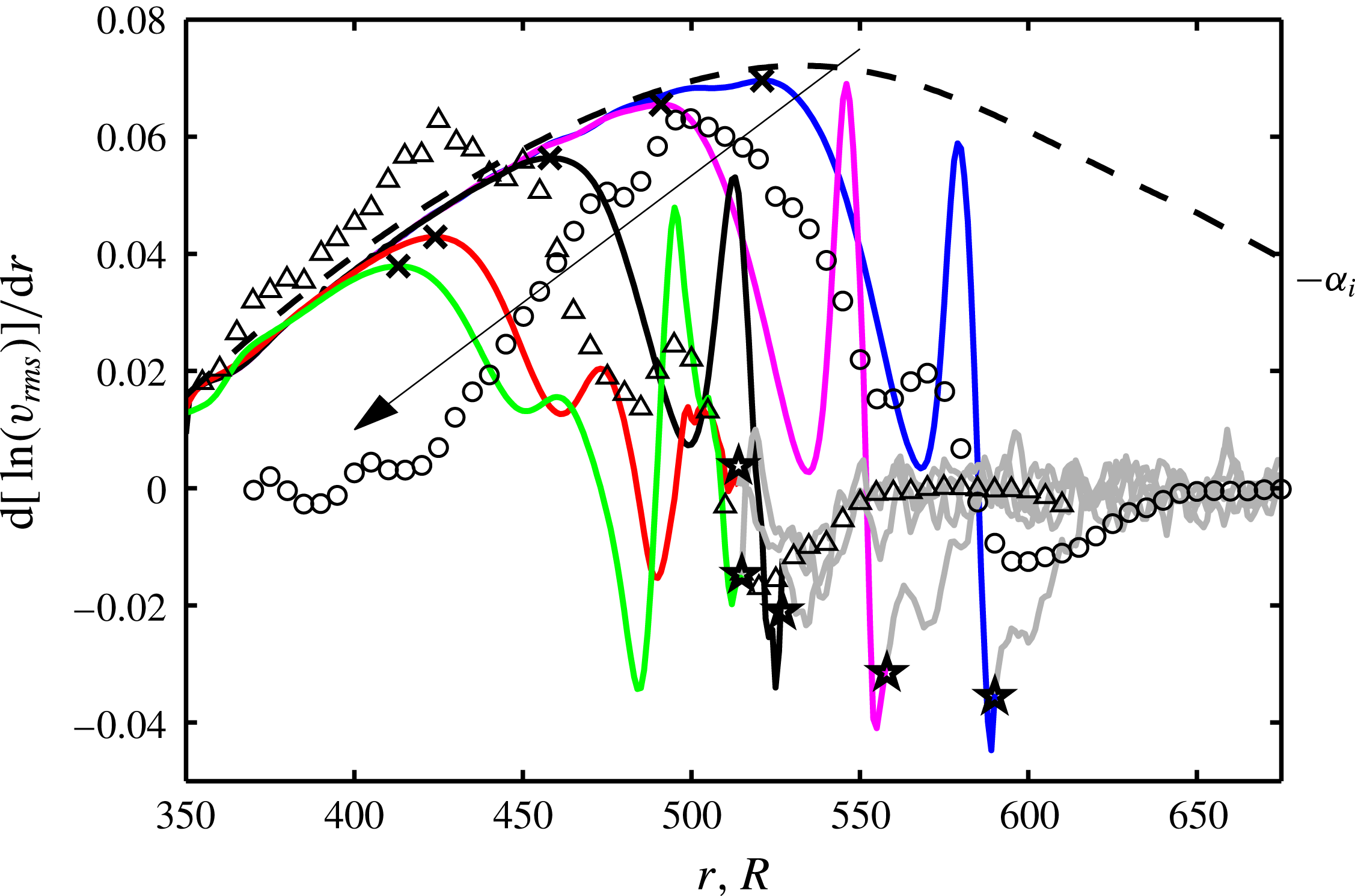
Figure 9. Growth rates of
 $v_{rms}$
are shown as a function of
$v_{rms}$
are shown as a function of
 $r$
for
$r$
for
 $z=1.3$
for simulations (at the final time) and experiments. An arrow gives the direction of simulations from A1 to A5, with the same colour keys as in figure 8. Markers are shown for deviation points (
$z=1.3$
for simulations (at the final time) and experiments. An arrow gives the direction of simulations from A1 to A5, with the same colour keys as in figure 8. Markers are shown for deviation points (
 $\times$
) and transition positions (
$\times$
) and transition positions (
 $\star$
) where the deviation points are denoted by maxima in the curves. The transition positions are defined in figure 14(b). The lines turn grey at the transition positions and are from here smoothed out by a running mean over five values. The dashed line shows the Type-I growth rates (
$\star$
) where the deviation points are denoted by maxima in the curves. The transition positions are defined in figure 14(b). The lines turn grey at the transition positions and are from here smoothed out by a running mean over five values. The dashed line shows the Type-I growth rates (
 $-\unicode[STIX]{x1D6FC}_{i}$
) for
$-\unicode[STIX]{x1D6FC}_{i}$
) for
 $\unicode[STIX]{x1D6FD}=32$
from local theory.
$\unicode[STIX]{x1D6FD}=32$
from local theory.
In figure 8(b) the experiments are seen to have a lower
 $v_{rms}$
amplitude than the simulations in the turbulent region. The hot-wire probe length for these experiments was 1 mm, which corresponds to almost 100 viscous units in the turbulent region leading to significant spatial resolution effects. In contrast, for the turbulent experiments by Imayama, Lingwood & Alfredsson (Reference Imayama, Lingwood and Alfredsson2014b
) the probe length was 0.3 mm. Using the data from that latter paper, one finds that at
$v_{rms}$
amplitude than the simulations in the turbulent region. The hot-wire probe length for these experiments was 1 mm, which corresponds to almost 100 viscous units in the turbulent region leading to significant spatial resolution effects. In contrast, for the turbulent experiments by Imayama, Lingwood & Alfredsson (Reference Imayama, Lingwood and Alfredsson2014b
) the probe length was 0.3 mm. Using the data from that latter paper, one finds that at
 $z=1.3$
(corresponding to
$z=1.3$
(corresponding to
 $z^{+}\approx 39$
)
$z^{+}\approx 39$
)
 $v_{rms}^{+}\approx 2.0$
, which yields
$v_{rms}^{+}\approx 2.0$
, which yields
 $v_{rms}\approx 0.089$
. That value is very close to the values obtained in our simulations.
$v_{rms}\approx 0.089$
. That value is very close to the values obtained in our simulations.
Figure 9 shows the spatial growth rate for the various cases and the theoretical linear growth rate of the Type-I mode
 $\unicode[STIX]{x1D6FD}=32$
as a dashed line. The simulation data are seen to follow the theoretical line closely until the vortices saturate and nonlinearities enter the flow. Also,
$\unicode[STIX]{x1D6FD}=32$
as a dashed line. The simulation data are seen to follow the theoretical line closely until the vortices saturate and nonlinearities enter the flow. Also,
 $\text{Exp}_{r}$
follows this dashed line well due to its 32 roughness elements. For case
$\text{Exp}_{r}$
follows this dashed line well due to its 32 roughness elements. For case
 $\text{Exp}_{c}$
there are many other wavenumbers present and their combined growth rate is therefore different from the theoretical line for
$\text{Exp}_{c}$
there are many other wavenumbers present and their combined growth rate is therefore different from the theoretical line for
 $\unicode[STIX]{x1D6FD}=32$
. The deviation points (
$\unicode[STIX]{x1D6FD}=32$
. The deviation points (
 $\times$
), defined as the radial location where the simulation data deviate from linear theory and reach a maximum growth rate (
$\times$
), defined as the radial location where the simulation data deviate from linear theory and reach a maximum growth rate (
 $r_{\times }$
), are listed in table 4. As expected, they are seen to be dependent on the amplitude of the forcing. This shows that the deviation points are in the convective region for the primary instability in line with the results of § 3.1. Downstream of the deviation points the growth rate decreases for all simulations until it reaches a minimum. Cases A4 and A5 have two well defined troughs before transition (around
$r_{\times }$
), are listed in table 4. As expected, they are seen to be dependent on the amplitude of the forcing. This shows that the deviation points are in the convective region for the primary instability in line with the results of § 3.1. Downstream of the deviation points the growth rate decreases for all simulations until it reaches a minimum. Cases A4 and A5 have two well defined troughs before transition (around
 $r=460$
and 490 in both cases) whereas cases A1–A3 only have one. The experimental data also experience troughs in the growth rate;
$r=460$
and 490 in both cases) whereas cases A1–A3 only have one. The experimental data also experience troughs in the growth rate;
 $\text{Exp}_{r}$
has two troughs in between its highest and lowest value, and
$\text{Exp}_{r}$
has two troughs in between its highest and lowest value, and
 $\text{Exp}_{c}$
experiences one, similar to cases
$\text{Exp}_{c}$
experiences one, similar to cases
 $\{\text{A4},\text{A5}\}$
and
$\{\text{A4},\text{A5}\}$
and
 $\{\text{A1},\text{A2},\text{A3}\}$
, respectively. This indicates that the transition scenarios for experiments and simulations agree and that there are two different observed scenarios. The transition position (
$\{\text{A1},\text{A2},\text{A3}\}$
, respectively. This indicates that the transition scenarios for experiments and simulations agree and that there are two different observed scenarios. The transition position (
 $r_{\star }$
) for each case is marked by a star and is defined later in figure 14(b) and it is also included in table 4.
$r_{\star }$
) for each case is marked by a star and is defined later in figure 14(b) and it is also included in table 4.
Table 4. Defined radial positions for cases A1–A5.

The two different observed transition scenarios are due to the role of the secondary instabilities. For cases A4 and A5, the first peak in figure 8(b) shows saturation of the primary stationary vortices. The second peak indicates the growth of secondary instabilities, this will be clarified in § 3.3.1. As already noted, cases A4, A5 and
 $\text{Exp}_{r}$
all have their highest
$\text{Exp}_{r}$
all have their highest
 $v_{rms}$
position close together (
$v_{rms}$
position close together (
 $r=515$
, 509 and 510, respectively) even though their initial disturbance amplitudes are quite different. This indicates a globally unstable dominated behaviour. The initial trigger of this globally unstable secondary instability can be related to the edge disturbances or the general development still occurring in the flow field at the time when the flow transitions to turbulence. For later times, the observed noise level in our DNS is low (figure 5
b) and will not trigger secondary convective instability. A globally unstable secondary instability can explain why all simulations become, and stay, turbulent without the introduction of disturbances continuously triggering secondary instabilities, and corresponds to the theory of Pier (Reference Pier2007) illustrated in figure 2. Both cases A4 and A5 then correspond to the grey curve in figure 2, case Ⓐ. The amplitude difference between the two simulations would make them saturate at different radial positions while becoming turbulent close together (position
$r=515$
, 509 and 510, respectively) even though their initial disturbance amplitudes are quite different. This indicates a globally unstable dominated behaviour. The initial trigger of this globally unstable secondary instability can be related to the edge disturbances or the general development still occurring in the flow field at the time when the flow transitions to turbulence. For later times, the observed noise level in our DNS is low (figure 5
b) and will not trigger secondary convective instability. A globally unstable secondary instability can explain why all simulations become, and stay, turbulent without the introduction of disturbances continuously triggering secondary instabilities, and corresponds to the theory of Pier (Reference Pier2007) illustrated in figure 2. Both cases A4 and A5 then correspond to the grey curve in figure 2, case Ⓐ. The amplitude difference between the two simulations would make them saturate at different radial positions while becoming turbulent close together (position
 $\hat{R}^{ca}$
from local theory and
$\hat{R}^{ca}$
from local theory and
 $R_{cgs}$
for our global simulation). The shorter transition region for case A4 (
$R_{cgs}$
for our global simulation). The shorter transition region for case A4 (
 $\unicode[STIX]{x0394}r_{\times \star }=90$
) compared to A5 (
$\unicode[STIX]{x0394}r_{\times \star }=90$
) compared to A5 (
 $\unicode[STIX]{x0394}r_{\times \star }=102$
) suggests such a behaviour. In contrast, cases A1, A2 and A3 correspond to the scenario represented by the black line in figure 2, case Ⓑ. Any small perturbation amplifies due to the already globally unstable secondary instability appearing as soon as the stationary vortices have saturated. The transition radial position is then dependent on the deviation point, from where the vortices saturate shortly downstream, and the transition scenario takes place over an average distance of
$\unicode[STIX]{x0394}r_{\times \star }=102$
) suggests such a behaviour. In contrast, cases A1, A2 and A3 correspond to the scenario represented by the black line in figure 2, case Ⓑ. Any small perturbation amplifies due to the already globally unstable secondary instability appearing as soon as the stationary vortices have saturated. The transition radial position is then dependent on the deviation point, from where the vortices saturate shortly downstream, and the transition scenario takes place over an average distance of
 $\unicode[STIX]{x0394}r_{\times \star }=68$
.
$\unicode[STIX]{x0394}r_{\times \star }=68$
.

Figure 10. The deformed mean flow (
 $\overline{V}_{N}$
) at
$\overline{V}_{N}$
) at
 $z=1.3$
for cases (a) A2 and (b) A5 shown in colour. The values are shown in linear scale where the azimuthal von Kármán velocity has a value of
$z=1.3$
for cases (a) A2 and (b) A5 shown in colour. The values are shown in linear scale where the azimuthal von Kármán velocity has a value of
 $-0.63$
for
$-0.63$
for
 $z=1.3$
. Black contours of the temporal r.m.s. values (
$z=1.3$
. Black contours of the temporal r.m.s. values (
 $v_{rms,t}$
) are shown on top in
$v_{rms,t}$
) are shown on top in
 $\log _{10}$
scale for values between
$\log _{10}$
scale for values between
 $-4$
to
$-4$
to
 $-0.5$
with a spacing of
$-0.5$
with a spacing of
 $\unicode[STIX]{x1D6E5}=0.5$
. In both panels, the simulation domain is shown twice in the azimuthal direction. The azimuthal direction is given by a dashed line, and both the streamwise and orthogonal plane to the stationary vortex are given by solid white lines.
$\unicode[STIX]{x1D6E5}=0.5$
. In both panels, the simulation domain is shown twice in the azimuthal direction. The azimuthal direction is given by a dashed line, and both the streamwise and orthogonal plane to the stationary vortex are given by solid white lines.
3.3 Secondary instability
3.3.1 Temporal disturbances
For the spatial development of the flow in the rotating reference frame, the time-averaged flow contains the stationary vortices, i.e. the new mean flow, and the r.m.s. in time indicates unsteady disturbances including secondary instabilities (if they are travelling with respect to the disk). The r.m.s. amplitudes of the azimuthal velocity normalized by the local disk velocity (
 $r\unicode[STIX]{x1D6FA}$
),
$r\unicode[STIX]{x1D6FA}$
),
 $V_{N}$
, are calculated in time
$V_{N}$
, are calculated in time
 $$\begin{eqnarray}\displaystyle v_{rms,t}(r,\unicode[STIX]{x1D703};z)=\sqrt{\frac{1}{T_{end}-T_{start}}\int _{T_{start}}^{T_{end}}(V_{N}-\overline{V}_{N})^{2}\,\text{d}t}, & & \displaystyle\end{eqnarray}$$
where
 $T_{start}$
and
$T_{start}$
and
 $T_{end}$
is the interval of the last half-rotation. The overbar defines the mean value in time.
$T_{end}$
is the interval of the last half-rotation. The overbar defines the mean value in time.
In figure 10 both the deformed mean flow (
 $\overline{V}_{N}$
) and r.m.s. in time (
$\overline{V}_{N}$
) and r.m.s. in time (
 $v_{rms,t}$
) are shown for cases A2 and A5 at
$v_{rms,t}$
) are shown for cases A2 and A5 at
 $z=1.3$
. The simulation domain is plotted twice in the azimuthal direction. The stationary vortices are clearly seen as coloured stripes across the domain in the azimuthal direction and the r.m.s. is shown with black contours on top. The streamwise and orthogonal plane to the stationary vortex are shown by solid lines for which data are shown later. The orthogonal plane, in the radial–vertical direction, is taken at an angle (
$z=1.3$
. The simulation domain is plotted twice in the azimuthal direction. The stationary vortices are clearly seen as coloured stripes across the domain in the azimuthal direction and the r.m.s. is shown with black contours on top. The streamwise and orthogonal plane to the stationary vortex are shown by solid lines for which data are shown later. The orthogonal plane, in the radial–vertical direction, is taken at an angle (
 $\unicode[STIX]{x1D700}$
) of 0.18 radians (
$\unicode[STIX]{x1D700}$
) of 0.18 radians (
 $10.3^{\circ }$
) to the azimuthal direction, shown as a dashed line. This is the average angle between the azimuthal and the vortex direction over the radial positions
$10.3^{\circ }$
) to the azimuthal direction, shown as a dashed line. This is the average angle between the azimuthal and the vortex direction over the radial positions
 $r=410{-}510$
which can be calculated by following equation (11) in Appelquist et al. (Reference Appelquist, Imayama, Alfredsson, Schlatter and Lingwood2016a
), which is the same as equation (1) in Wilkinson & Malik (Reference Wilkinson and Malik1985):
$r=410{-}510$
which can be calculated by following equation (11) in Appelquist et al. (Reference Appelquist, Imayama, Alfredsson, Schlatter and Lingwood2016a
), which is the same as equation (1) in Wilkinson & Malik (Reference Wilkinson and Malik1985):
 $$\begin{eqnarray}\displaystyle \text{tan}\,\unicode[STIX]{x1D700}=\frac{1}{r}\left.\frac{\text{d}r}{\text{d}\unicode[STIX]{x1D703}}\right|_{s}, & & \displaystyle\end{eqnarray}$$
where
 $s(r,\unicode[STIX]{x1D703})$
is the radial locus of the vortex.
$s(r,\unicode[STIX]{x1D703})$
is the radial locus of the vortex.
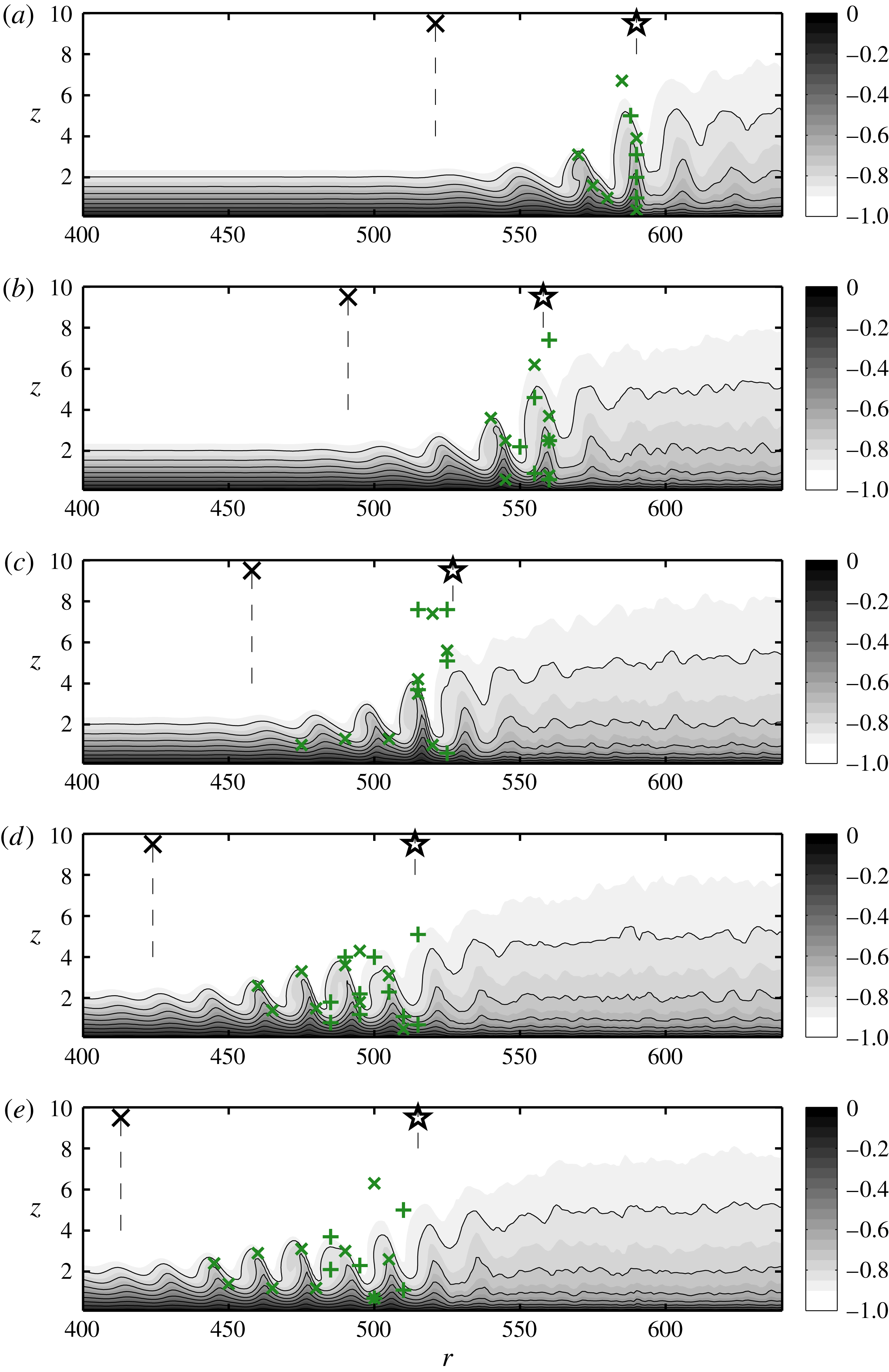
Figure 11. The deformed mean flow (
 $\overline{V}_{N}$
) with zero velocity at the wall increasing to a negative one in the free stream. Black lines are shown for
$\overline{V}_{N}$
) with zero velocity at the wall increasing to a negative one in the free stream. Black lines are shown for
 $\unicode[STIX]{x1D6E5}=0.1$
contours from
$\unicode[STIX]{x1D6E5}=0.1$
contours from
 $-0.8$
to zero. Vertical dashed lines are seen connected to a marker representing the deviation points (
$-0.8$
to zero. Vertical dashed lines are seen connected to a marker representing the deviation points (
 $\boldsymbol{\times }$
) or transition position (
$\boldsymbol{\times }$
) or transition position (
 $\star$
). Markers
$\star$
). Markers
 $\times$
and
$\times$
and
 $+$
are used for indicating the secondary instabilities in the flow field: (a) A1; (b) A2; (c) A3; (d) A4; (e) A5.
$+$
are used for indicating the secondary instabilities in the flow field: (a) A1; (b) A2; (c) A3; (d) A4; (e) A5.
The deformed mean flow (
 $\overline{V}_{N}$
) is shown in figure 11 along the orthogonal plane given by the white dashed line in figure 10. Note that the velocities are not rotated according to the line. Simulations A1–A5 are shown in figures 11(a–e) and the deviation and transition positions (table 4) are shown as vertical dashed lines connected to the marker,
$\overline{V}_{N}$
) is shown in figure 11 along the orthogonal plane given by the white dashed line in figure 10. Note that the velocities are not rotated according to the line. Simulations A1–A5 are shown in figures 11(a–e) and the deviation and transition positions (table 4) are shown as vertical dashed lines connected to the marker,
 $\times$
and
$\times$
and
 $\star$
, respectively. There are also markers that indicate locations of a maximum of secondary instabilities of the flow field when decomposed into Fourier modes. There are two kinds marked with
$\star$
, respectively. There are also markers that indicate locations of a maximum of secondary instabilities of the flow field when decomposed into Fourier modes. There are two kinds marked with
 $\times$
or
$\times$
or
 $+$
for low and high frequency maxima with temporal frequencies 28 and 156, respectively. In figure 11 it can be seen that cases A4 and A5 have longer transition regions (
$+$
for low and high frequency maxima with temporal frequencies 28 and 156, respectively. In figure 11 it can be seen that cases A4 and A5 have longer transition regions (
 $\unicode[STIX]{x0394}r_{\times \star }$
) compared with cases A1, A2 and A3. Also, the similarity between the latter three cases (a–c) reflects a similar transition scenario. Additional data for cases A2 and A5 are shown in figure 12. The panels show the amplitude of
$\unicode[STIX]{x0394}r_{\times \star }$
) compared with cases A1, A2 and A3. Also, the similarity between the latter three cases (a–c) reflects a similar transition scenario. Additional data for cases A2 and A5 are shown in figure 12. The panels show the amplitude of
 $\overline{V_{N}}$
as wall-normal profiles at equidistant
$\overline{V_{N}}$
as wall-normal profiles at equidistant
 $r$
-positions. For case A2 the profiles are taken over
$r$
-positions. For case A2 the profiles are taken over
 $r=545{-}560$
, which consist of one deformed wave seen in 11(b) whereafter the flow becomes turbulent. This radial range spans over the high-amplitude peak seen in figure 8. For case A5 the wall-normal profiles in figure 12(b) are taken over
$r=545{-}560$
, which consist of one deformed wave seen in 11(b) whereafter the flow becomes turbulent. This radial range spans over the high-amplitude peak seen in figure 8. For case A5 the wall-normal profiles in figure 12(b) are taken over
 $r=465{-}480$
, which consist of one deformed wave seen in 11(e). This radial range spans over the peak with smallest
$r=465{-}480$
, which consist of one deformed wave seen in 11(e). This radial range spans over the peak with smallest
 $r$
seen in figure 8. In figure 12(b) three profiles are marked, corresponding to positions where the lowest-frequency (
$r$
seen in figure 8. In figure 12(b) three profiles are marked, corresponding to positions where the lowest-frequency (
 $\times$
) peaks at the bottom (
$\times$
) peaks at the bottom (
 $r=465$
and 480), and at the top (
$r=465$
and 480), and at the top (
 $r=475$
). It can be seen that the initial and final wave profile are similar. For the top peak, one of the most deformed mean flow profiles is seen.
$r=475$
). It can be seen that the initial and final wave profile are similar. For the top peak, one of the most deformed mean flow profiles is seen.
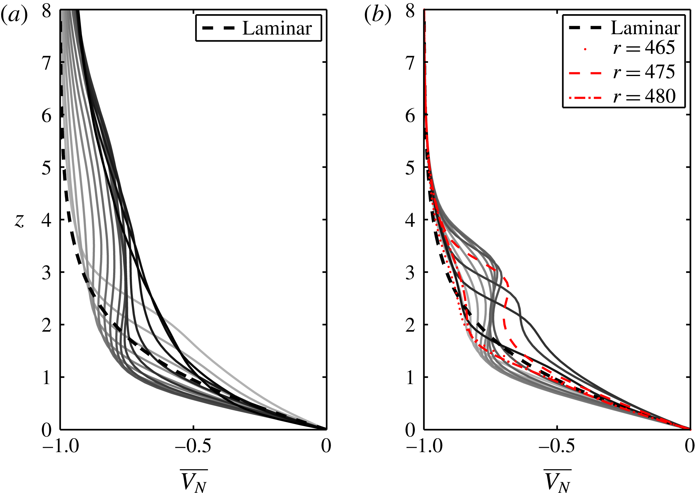
Figure 12. Wall-normal profiles of the deformed mean flow
 $\overline{V_{N}}$
(time averaged) for (a) case A2 over
$\overline{V_{N}}$
(time averaged) for (a) case A2 over
 $r=545{-}560$
where darker shade indicates larger radial position and (b) for A5 over
$r=545{-}560$
where darker shade indicates larger radial position and (b) for A5 over
 $r=465{-}480$
. The dashed black lines correspond to the von Kármán profile.
$r=465{-}480$
. The dashed black lines correspond to the von Kármán profile.
Figure 13 shows the deformation of the mean flow as black and white contours obtained by subtracting the laminar von Kármán solution from the averaged field. On top of this the
 $v_{rms,t}$
(3.1) is shown. Also vertical dashed lines and markers are shown as in figure 11. In figure 13, it is possible to see that the positions of the markers, i.e. secondary instabilities, lie on high values of temporal r.m.s. as expected. The deformation of the mean flow for case A5 starts at smaller
$v_{rms,t}$
(3.1) is shown. Also vertical dashed lines and markers are shown as in figure 11. In figure 13, it is possible to see that the positions of the markers, i.e. secondary instabilities, lie on high values of temporal r.m.s. as expected. The deformation of the mean flow for case A5 starts at smaller
 $r$
than for case A4, which is reasonable due to the higher amplitude of the crossflow vortices however the r.m.s. values in colour start approximately at the same radius.
$r$
than for case A4, which is reasonable due to the higher amplitude of the crossflow vortices however the r.m.s. values in colour start approximately at the same radius.

Figure 13. Showing
 $v_{rms,t}$
in colour
$v_{rms,t}$
in colour
 $\log _{10}$
scale and the deformation of the mean flow in black (negative values) and white (positive values). Zero contour is not included. The contour spacing is
$\log _{10}$
scale and the deformation of the mean flow in black (negative values) and white (positive values). Zero contour is not included. The contour spacing is
 $\unicode[STIX]{x1D6E5}=0.05$
. Vertical dashed lines and markers are included as in figure 11: (a) A1; (b) A2; (c) A3; (d) A4; (e) A5.
$\unicode[STIX]{x1D6E5}=0.05$
. Vertical dashed lines and markers are included as in figure 11: (a) A1; (b) A2; (c) A3; (d) A4; (e) A5.
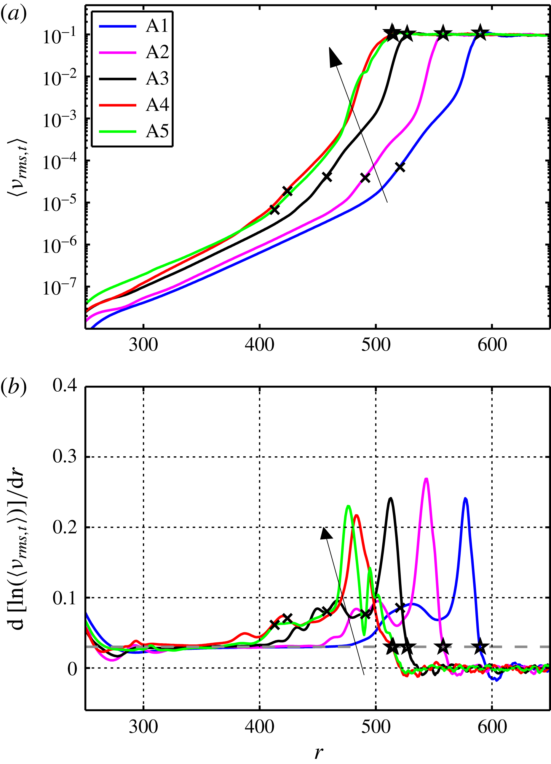
Figure 14. Averaged
 $v_{rms,t}$
in the azimuthal direction to obtain the growth and growth rate of the secondary disturbances at
$v_{rms,t}$
in the azimuthal direction to obtain the growth and growth rate of the secondary disturbances at
 $z=1.3$
. The positions in table 4 are shown and a grey dashed line is included in (b) to show the definition of the transition position. Arrows show the lines for cases A1 to A5.
$z=1.3$
. The positions in table 4 are shown and a grey dashed line is included in (b) to show the definition of the transition position. Arrows show the lines for cases A1 to A5.
Estimating the growth rates of all secondary instabilities also shows similar behaviour for cases A4 and A5. The temporal r.m.s.,
 $v_{rms,t}$
, averaged in the azimuthal direction together with its radial growth rate are shown in figure 14. Since
$v_{rms,t}$
, averaged in the azimuthal direction together with its radial growth rate are shown in figure 14. Since
 $v_{rms,t}$
indicates unsteady disturbances including secondary instabilities the figure shows a collection of all these present in the flow but excludes stationary disturbances. In figure 14(a), both curves of A4 and A5 are seen to follow each other closely. For these cases, the
$v_{rms,t}$
indicates unsteady disturbances including secondary instabilities the figure shows a collection of all these present in the flow but excludes stationary disturbances. In figure 14(a), both curves of A4 and A5 are seen to follow each other closely. For these cases, the
 $\langle v_{rms,t}\rangle$
amplitude for
$\langle v_{rms,t}\rangle$
amplitude for
 $r<485$
is below
$r<485$
is below
 $10^{-2}$
, hence the
$10^{-2}$
, hence the
 $v_{rms}$
peak in figure 8 of magnitude
$v_{rms}$
peak in figure 8 of magnitude
 $10^{-1}$
at these
$10^{-1}$
at these
 $r$
must be due to stationary disturbances. The radial position of the second peak occurring around
$r$
must be due to stationary disturbances. The radial position of the second peak occurring around
 $r=510$
in figure 8 corresponds, however, well to the amplitude level of the secondary temporal disturbances shown in figure 14(b). Also, Imayama et al. (Reference Imayama, Alfredsson and Lingwood2014a
) (
$r=510$
in figure 8 corresponds, however, well to the amplitude level of the secondary temporal disturbances shown in figure 14(b). Also, Imayama et al. (Reference Imayama, Alfredsson and Lingwood2014a
) (
 $\text{Exp}_{c}$
) could see a rapid growth in high-frequency disturbances for
$\text{Exp}_{c}$
) could see a rapid growth in high-frequency disturbances for
 $R=565{-}590$
, which agrees with case A1. The noise level was previously shown in figure 5(b) and is well below the
$R=565{-}590$
, which agrees with case A1. The noise level was previously shown in figure 5(b) and is well below the
 $\langle v_{rms,t}\rangle$
values. An additional simulation including a trip forcing but otherwise similar to case A3 was undertaken. There was an increase in the noise level for this simulation however no change with regards to the transition scenario occurred. For the growth rates shown in figure 14(b) growth is seen upstream of the highest peak. There is no clear dependence of this growth in relation to the convective behaviour of the primary disturbances such as the deviation point. It is possible that this growth is induced by the downstream transition triggering upstream modes. Moreover the values in figure 14(b) reach around four times higher than the maximum values in figure 9 for the maximum primary amplification. Also in figure 14(b) a grey dashed line at 0.03 indicates a definition of the transition position for each simulation given in table 4. This threshold is chosen just before the growth rates go to an average of zero, such that the transition position marks the beginning of the plateau for each curve in figure 14(a). This position is similar for cases A4 and A5, and along with the similar curves this shows a co-location of transition for the two cases, which is a result of the global secondary instability at
$\langle v_{rms,t}\rangle$
values. An additional simulation including a trip forcing but otherwise similar to case A3 was undertaken. There was an increase in the noise level for this simulation however no change with regards to the transition scenario occurred. For the growth rates shown in figure 14(b) growth is seen upstream of the highest peak. There is no clear dependence of this growth in relation to the convective behaviour of the primary disturbances such as the deviation point. It is possible that this growth is induced by the downstream transition triggering upstream modes. Moreover the values in figure 14(b) reach around four times higher than the maximum values in figure 9 for the maximum primary amplification. Also in figure 14(b) a grey dashed line at 0.03 indicates a definition of the transition position for each simulation given in table 4. This threshold is chosen just before the growth rates go to an average of zero, such that the transition position marks the beginning of the plateau for each curve in figure 14(a). This position is similar for cases A4 and A5, and along with the similar curves this shows a co-location of transition for the two cases, which is a result of the global secondary instability at
 $R_{cgs}$
.
$R_{cgs}$
.
3.3.2 Fourier decomposition
Scrutinizing the fluctuations in time further, the velocity signal was decomposed into Fourier modes. Figure 15 shows the (square root of the) energy content of these modes (
 $\unicode[STIX]{x1D714}<200$
) as a function of
$\unicode[STIX]{x1D714}<200$
) as a function of
 $r$
at height
$r$
at height
 $z=1.3$
for simulations A2 and A5 together with their growth rate in
$z=1.3$
for simulations A2 and A5 together with their growth rate in
 $r$
. Similarities to figure 14 can be observed. The maximum growth rates for both cases involve the highest frequencies where
$r$
. Similarities to figure 14 can be observed. The maximum growth rates for both cases involve the highest frequencies where
 $\unicode[STIX]{x1D714}=156$
is chosen and marked with a thick line. For smaller radial positions,
$\unicode[STIX]{x1D714}=156$
is chosen and marked with a thick line. For smaller radial positions,
 $\unicode[STIX]{x1D714}=28$
is larger and marked with a dashed line. Both of these frequencies were chosen from among the strongest growing frequencies for all cases and were, therefore, regarded as representative for all cases and were further analysed in space. As stated earlier, the low-frequency mode (
$\unicode[STIX]{x1D714}=28$
is larger and marked with a dashed line. Both of these frequencies were chosen from among the strongest growing frequencies for all cases and were, therefore, regarded as representative for all cases and were further analysed in space. As stated earlier, the low-frequency mode (
 $\unicode[STIX]{x1D714}=28$
) maxima are marked by
$\unicode[STIX]{x1D714}=28$
) maxima are marked by
 $\times$
(cross-mode) in figures 11 and 13. The growth rate of this mode decreases when the higher-frequency mode (
$\times$
(cross-mode) in figures 11 and 13. The growth rate of this mode decreases when the higher-frequency mode (
 $\unicode[STIX]{x1D714}=156$
) appears, and its maxima are marked by
$\unicode[STIX]{x1D714}=156$
) appears, and its maxima are marked by
 $+$
(plus mode) in figures 11 and 13. The peaks of the two modes are only marked for
$+$
(plus mode) in figures 11 and 13. The peaks of the two modes are only marked for
 $r$
smaller than the transition position and for a threshold of
$r$
smaller than the transition position and for a threshold of
 $10^{-5}$
. In the same figures it can be seen that the cross mode prefers to be either at high or low vertical positions on the stationary vortex.
$10^{-5}$
. In the same figures it can be seen that the cross mode prefers to be either at high or low vertical positions on the stationary vortex.

Figure 15. The energy content of modes
 $\unicode[STIX]{x1D714}<200$
,
$\unicode[STIX]{x1D714}<200$
,
 $\unicode[STIX]{x1D714}=28$
(- - -) and
$\unicode[STIX]{x1D714}=28$
(- - -) and
 $\unicode[STIX]{x1D714}=156$
(——), taken from a signal along a radial line such as in figure 10 at
$\unicode[STIX]{x1D714}=156$
(——), taken from a signal along a radial line such as in figure 10 at
 $z=1.3$
. The picture was similar for all heights: (a) A2; (b) A2; (c) A5; (d) A5.
$z=1.3$
. The picture was similar for all heights: (a) A2; (b) A2; (c) A5; (d) A5.


In figures 16 and 17 the
 $z$
and
$z$
and
 $r$
gradients, respectively, of the deformed mean flow are shown, again for simulations (a) A1–(e) A5. Also, here the maxima of the two modes are marked (
$r$
gradients, respectively, of the deformed mean flow are shown, again for simulations (a) A1–(e) A5. Also, here the maxima of the two modes are marked (
 $\times$
and
$\times$
and
 $+$
), and the cross-mode at high vertical positions (top) can be connected to a large negative
$+$
), and the cross-mode at high vertical positions (top) can be connected to a large negative
 $z$
-gradient and at low vertical positions (bottom) can similarly be connected to a large negative
$z$
-gradient and at low vertical positions (bottom) can similarly be connected to a large negative
 $r$
-gradient. This is most easily seen for case A4 and A5 where the cross-mode has a larger range. As shown by Malik et al. (Reference Malik, Li, Choudhari and Chang1999) secondary modes are generated where there are high gradients in the mean flow, these are associated with the disturbance energy production. The plus mode is seen to be in the neighbourhood of the cross-mode for cases A4 and A5, and may be dependent on the additional shear this mode creates since it is difficult to connect this mode to the shear of the mean flow. As seen for case A1, it is possible to find all markers very close to the transition position, where they collect on a vertical line at
$r$
-gradient. This is most easily seen for case A4 and A5 where the cross-mode has a larger range. As shown by Malik et al. (Reference Malik, Li, Choudhari and Chang1999) secondary modes are generated where there are high gradients in the mean flow, these are associated with the disturbance energy production. The plus mode is seen to be in the neighbourhood of the cross-mode for cases A4 and A5, and may be dependent on the additional shear this mode creates since it is difficult to connect this mode to the shear of the mean flow. As seen for case A1, it is possible to find all markers very close to the transition position, where they collect on a vertical line at
 $r=590$
.
$r=590$
.
3.3.3 Experimental comparison
Further comparing the simulations to experiments, azimuthal velocity signals from case A5 are shown in figure 18(a–c) where they are normalized to an amplitude of one. In (a) the signal shows both the low and high-frequency modes in the rotating frame of reference. This is because in the specific position chosen (
 $r=500$
and
$r=500$
and
 $z=0.7$
, see markers in figures 11, 13, 16 and 17) both modes are strong. In the laboratory frame of reference, (b), the flow is also modulated by the stationary vortex. The reason for shifting into this frame is to compare with experiments, where the transition route seen in figure 7 of Kobayashi et al. (Reference Kobayashi, Kohama and Takamadate1980) is concluded in Imayama et al. (Reference Imayama, Alfredsson and Lingwood2013) to be a convective route. Imayama et al. (Reference Imayama, Alfredsson and Lingwood2013) reinterpret the transition Reynolds number to be
$z=0.7$
, see markers in figures 11, 13, 16 and 17) both modes are strong. In the laboratory frame of reference, (b), the flow is also modulated by the stationary vortex. The reason for shifting into this frame is to compare with experiments, where the transition route seen in figure 7 of Kobayashi et al. (Reference Kobayashi, Kohama and Takamadate1980) is concluded in Imayama et al. (Reference Imayama, Alfredsson and Lingwood2013) to be a convective route. Imayama et al. (Reference Imayama, Alfredsson and Lingwood2013) reinterpret the transition Reynolds number to be
 $R<500$
. Also, for our simulation, A5 has a transition Reynolds number
$R<500$
. Also, for our simulation, A5 has a transition Reynolds number
 $R<500$
due to nonlinearities entering the flow field upstream of this position. Comparing the oscillogram of velocity fluctuations in figure 9(d) of Kobayashi et al. (Reference Kobayashi, Kohama and Takamadate1980) to our figure 18(c) for
$R<500$
due to nonlinearities entering the flow field upstream of this position. Comparing the oscillogram of velocity fluctuations in figure 9(d) of Kobayashi et al. (Reference Kobayashi, Kohama and Takamadate1980) to our figure 18(c) for
 $R=500$
and
$R=500$
and
 $z=1.8$
, clear similarities can be seen. Additionally, emphasizing the similarities to experiments, the striped pattern seen in flow visualizations, e.g. figure 8 by Kobayashi et al. (Reference Kobayashi, Kohama and Takamadate1980), can be found in our simulations as shown in figure 6(b). The stripes were, however, only clear for cases A4 and A5 prior to the secondary global instability due the turbulent breakdown this initiates.
$z=1.8$
, clear similarities can be seen. Additionally, emphasizing the similarities to experiments, the striped pattern seen in flow visualizations, e.g. figure 8 by Kobayashi et al. (Reference Kobayashi, Kohama and Takamadate1980), can be found in our simulations as shown in figure 6(b). The stripes were, however, only clear for cases A4 and A5 prior to the secondary global instability due the turbulent breakdown this initiates.
Figure 18. Azimuthal velocity signals normalized to unit maximum amplitude for specified heights at
 $r=500$
from case A5. The position is specified to be on the white solid line orthogonal to the vortex direction in figure 10(b). (a)
$r=500$
from case A5. The position is specified to be on the white solid line orthogonal to the vortex direction in figure 10(b). (a)
 $z=0.7$
, rotating frame of reference; (b)
$z=0.7$
, rotating frame of reference; (b)
 $z=0.7$
, laboratory frame of reference; (c)
$z=0.7$
, laboratory frame of reference; (c)
 $z=1.8$
, laboratory frame of reference.
$z=1.8$
, laboratory frame of reference.
3.4 Comparison with secondary instabilities of the swept-wing flow
The cross-flow instabilities arising on the rotating-disk and the swept-wing boundary-layer flows have been compared since the early studies by Gregory, Stuart & Walker (Reference Gregory, Stuart and Walker1955). The boundary layer developing on the rotating disk can be viewed as an idealized case of the swept-wing boundary-layer flow, for which there is only one control parameter to take into account, viz. the Reynolds number. When setting up an experiment, in the case of a swept-wing flow one must decide what sweep angle, free-stream velocity as well as pressure gradient to use; the latter given by the wing geometry and angle of attack. In the case of the rotating disk, the only decision is what Reynolds number range to study and choose the disk diameter and rotational speed range appropriately. The rotating-disk flow also has the advantage that the velocity distribution in the laminar boundary layer is well known from the similarity solution. Furthermore, results from the rotating-disk boundary layer are naturally normalized by the disk speed, which makes comparisons for different radial positions (i.e. Reynolds numbers) straightforward.
There are, however, differences between the two cases such as the azimuthal periodicity for the disk, which does not exist for the wing. Also, for the disk, the shear-layer thickness is constant in the laminar case in contrast to the wing, and the strength of the cross-flow is constant relative to the disk velocity (free stream). For the swept wing this relative strength increases. These differences might result in the nature of the instabilities in the two flows differing. For the rotating disk the boundary layer experiences a global instability (Appelquist et al. Reference Appelquist, Schlatter, Alfredsson and Lingwood2016b ) and for the swept wing it is convective (Wassermann & Kloker Reference Wassermann and Kloker2002). Also as shown here, the secondary instability experiences a global instability unlike observations for the wing. For similar simulations over the swept wing (Högberg & Henningson Reference Högberg and Henningson1998; Wassermann & Kloker Reference Wassermann and Kloker2002; Hosseini et al. Reference Hosseini, Tempelmann, Hanifi and Henningson2013), additional low-level disturbances were needed to excite the secondary instability causing transition.
For a brief comparison of the secondary instabilities in the two boundary layers, the high-frequency plus mode found here can be compared to the low-frequency mode in Wassermann & Kloker (Reference Wassermann and Kloker2002), which relies on the energy production related to the shear of their high-frequency mode. The high growth rate of the plus mode is also similar to theirs. The low-frequency cross-mode for the disk can further be related to the high-frequency mode in Wassermann & Kloker (Reference Wassermann and Kloker2002). This mode is classified as a ‘z’-mode, which would correspond to an ‘r’-mode for our case. For the wing, it has its maximum amplitude located on the back of the wave, relating to a maximum of the negative spanwise gradient. In our case, this corresponds to a negative
 $r$
-gradient as found for the cross-mode maxima close to the wall. The top of the cross-mode gives a large deformed mean flow profile as shown in figure 12(b) (
$r$
-gradient as found for the cross-mode maxima close to the wall. The top of the cross-mode gives a large deformed mean flow profile as shown in figure 12(b) (
 $r=475$
), and a similar profile is found in Wassermann & Kloker’s (Reference Wassermann and Kloker2002) figure 10(b) to be the most deformed in a similar location on the wave.
$r=475$
), and a similar profile is found in Wassermann & Kloker’s (Reference Wassermann and Kloker2002) figure 10(b) to be the most deformed in a similar location on the wave.
Further research comparing swept-wing and rotating-disk flows should be undertaken to determine the structure and frequencies of the secondary instabilities. For the rotating-disk boundary-layer flow the simulations should then be focused on a region prior to the secondary global instability, such that the secondary instabilities can grow and fully develop in the field.
4 Conclusions
In the present study,
 $1/32$
of a rotating disk is simulated and the primary global instability is determined to be located at
$1/32$
of a rotating disk is simulated and the primary global instability is determined to be located at
 $R_{cg}=599$
for an azimuthal wavenumber
$R_{cg}=599$
for an azimuthal wavenumber
 $\unicode[STIX]{x1D6FD}=64$
. All simulations including a stationary disturbance become turbulent before
$\unicode[STIX]{x1D6FD}=64$
. All simulations including a stationary disturbance become turbulent before
 $R_{cg}$
and are therefore considered to be convectively unstable with respect to the primary instability. This convective behaviour is also shown by the defined deviation point, which directly depends on the amplitude of the initial disturbance. Nonlinear waves develop downstream of the deviation point and secondary instabilities grow on top of these waves. Two categories of behaviour have been identified based on the amplitude of disturbances and the behaviour of the secondary instability; these are illustrated in figure 2. Ⓐ represents a category where the primary instability is susceptible to secondary instabilities before the radial position for secondary global instability (
$R_{cg}$
and are therefore considered to be convectively unstable with respect to the primary instability. This convective behaviour is also shown by the defined deviation point, which directly depends on the amplitude of the initial disturbance. Nonlinear waves develop downstream of the deviation point and secondary instabilities grow on top of these waves. Two categories of behaviour have been identified based on the amplitude of disturbances and the behaviour of the secondary instability; these are illustrated in figure 2. Ⓐ represents a category where the primary instability is susceptible to secondary instabilities before the radial position for secondary global instability (
 $R_{cgs}$
) and, therefore, transition undergoes at the point of secondary global instability. Ⓑ represents the second category that, in contrast, becomes turbulent as soon as the primary instability has grown enough to become susceptible to secondary global instabilities; this is due to the flow already being globally unstable at the saturation position. In particular, figure 6(a,b) shows these two transition scenarios where the flow saturates for small radial positions in (a) for case A5, Ⓐ, and carries visible secondary instabilities. In (b) the flow instead saturates for large radial positions for case A2, showing an unstable behaviour where it is possible to see a black region widening at
$R_{cgs}$
) and, therefore, transition undergoes at the point of secondary global instability. Ⓑ represents the second category that, in contrast, becomes turbulent as soon as the primary instability has grown enough to become susceptible to secondary global instabilities; this is due to the flow already being globally unstable at the saturation position. In particular, figure 6(a,b) shows these two transition scenarios where the flow saturates for small radial positions in (a) for case A5, Ⓐ, and carries visible secondary instabilities. In (b) the flow instead saturates for large radial positions for case A2, showing an unstable behaviour where it is possible to see a black region widening at
 $r=550$
as the secondary instability is amplified globally.
$r=550$
as the secondary instability is amplified globally.
The initial triggering of the globally unstable secondary instabilities for both categories is likely to be related to edge disturbances or the initial development of the flow field. High-frequency secondary instabilities are then amplified where the global instability appears causing rapid breakdown. These high-frequency modes grow suddenly with a high growth rate and are named here as plus modes. The secondary global instability trips the flow upstream causing low-frequency secondary instabilities, so-called cross-modes at lower Reynolds numbers. This cross-mode is localized in physical space and relates to the structure of the primary vortices, where it occurs on the lower back and on top of the wave related to the large shear of the deformed mean flow in the
 $r$
- and
$r$
- and
 $z$
-direction, respectively. The cross-mode (
$z$
-direction, respectively. The cross-mode (
 $\times$
) is positioned on the lower back of the primary vortex can also be related to a high-frequency mode for the swept-wing flow (e.g. Wassermann & Kloker Reference Wassermann and Kloker2002).
$\times$
) is positioned on the lower back of the primary vortex can also be related to a high-frequency mode for the swept-wing flow (e.g. Wassermann & Kloker Reference Wassermann and Kloker2002).
The simulations were set-up for a finite domain such that a comparison to experiments could be made directly. The transition scenarios have been shown to agree well. Also, similarities were directly found between our simulations and the experiments by Kobayashi et al. (Reference Kobayashi, Kohama and Takamadate1980). The present analysis appears sufficient to show that the secondary instability is globally unstable. It could, however, be interesting to verify the results by a linear stability analysis of the saturated nonlinear waves and to extend the investigations of the latter to more than a single azimuthal wavenumber and to non-stationary primary vortices. A shift of either the wavenumber or the frequency would shift the transition position due to a change in the baseflow however we expect the two transition scenarios to be qualitatively similar to those described here. Judicious choices of azimuthal wavenumber and harmonic forcing frequency could give the opportunity to control the flow (Pier Reference Pier2007). Furthermore, a question that arises is whether the critical position of the secondary global instability (i.e. the lowest value of
 $R$
across all
$R$
across all
 $\unicode[STIX]{x1D6FD}$
) collapses on to the critical absolute instability position of the primary disturbance. For
$\unicode[STIX]{x1D6FD}$
) collapses on to the critical absolute instability position of the primary disturbance. For
 $\unicode[STIX]{x1D6FD}=64$
this would give
$\unicode[STIX]{x1D6FD}=64$
this would give
 $R_{cgs}=R_{c}=510$
close to the peak amplitude of the secondary instability for cases A4, A5 and
$R_{cgs}=R_{c}=510$
close to the peak amplitude of the secondary instability for cases A4, A5 and
 $\text{Exp}_{r}$
.
$\text{Exp}_{r}$
.
To finally conclude the paper and to summarize the understanding so far on the rotating-disk boundary-layer flow, the following stability and transition regions have been identified:
-
(i) For
 $R<49$
(Malik, Wilkinson & Orszag Reference Malik, Wilkinson and Orszag1981) the flow does not admit exponentially growing instabilities.
$R<49$
(Malik, Wilkinson & Orszag Reference Malik, Wilkinson and Orszag1981) the flow does not admit exponentially growing instabilities. -
(ii) For
$49<R<R_{cgs}$
the flow is convectively unstable both for the primary and secondary instability. The secondary global instability position,
$R_{cgs}$
, is dependent on the azimuthal wavenumber and the frequency of the primary nonlinear waves. -
(iii) At
$R_{cgs}$
, around
$r=510$
for
$\unicode[STIX]{x1D6FD}=32$
(stationary vortices), the flow allows secondary global instability such that disturbances on top of the saturated vortices trigger a sudden transition to turbulence. -
(iv) For
$R_{cgs}<R<R_{cg}$
the flow is globally unstable to secondary instabilities. -
(v) At
$R_{cg}$
the flow becomes globally unstable to the primary instability.


The above applies not only to stationary vortices in a finite domain but also to travelling waves. The finding of the secondary global instability finally gives an answer to why the rotating-disk boundary-layer flow has such a sharp transition to turbulence.
Acknowledgements
This work is supported by the Swedish Research Council through the ASTRID project and the Linné FLOW Centre. Computer time was provided by the Swedish National Infrastructure for Computing (SNIC). Dr S. Imayama is gratefully acknowledged for providing data from rotating-disk experiments. Dr B. Pier is also acknowledged for fruitful discussions.


