


1 Introduction
Turbulent bubble fountains form when gas bubbles are carried into a liquid by a downward jet of water. They frequently arise in industrial processes, most commonly in the form of air bubbles entering a liquid reservoir. Two-phase fountains can be highly desirable when aerating oxygen-scarce water (McDougall Reference McDougall1978; Biń Reference Biń1993), or highly undesirable when contamination of the liquid with bubbles is to be avoided. Examples of the latter case include the foaming induced when refuelling a petrol tank and the entrainment of air into oil as it refills the sump of an engine. In particular connecting-rod bearings in car engines show increased wear when the lubricant is laden with bubbles (Nemoto et al. Reference Nemoto, Kawata, Kuribayashii, Akiyama, Kawai and Murakawai1997). The purpose of this work is to broaden our understanding of bubble fountains and in particular the controls on the penetration depth of the bubbles.
We present a new set of systematic experiments in which we generate turbulent bubble fountains via a co-flow of air and fresh water issuing through a submerged nozzle. This set-up allows for a precise control of both the air and water flow rates at the source. We explore scalings for our experimental measurements of bubble penetration depth in terms of the initial fluxes of volume, momentum and buoyancy and present an integral model which describes how these horizontally averaged fluxes develop in the vertical direction. The model quantifies the effect of the bubble slip velocity,
 $u_{slip}$
(the terminal rise speed of an individual air bubble in water), on the fountain dynamics and quantifies the mixing with ambient liquid. Comparison of the model with experimental data yields a best-fit entrainment coefficient,
$u_{slip}$
(the terminal rise speed of an individual air bubble in water), on the fountain dynamics and quantifies the mixing with ambient liquid. Comparison of the model with experimental data yields a best-fit entrainment coefficient,
 $\unicode[STIX]{x1D6FC}$
. The model predictions for bubble penetration distance are in good accord with the new experimental data.
$\unicode[STIX]{x1D6FC}$
. The model predictions for bubble penetration distance are in good accord with the new experimental data.
Our experiments build on existing literature about bubble fountains generated by plunging water jets (Biń Reference Biń1993), for which a constant bubble slip velocity has been observed (Clanet & Lasheras Reference Clanet and Lasheras1997). In contrast to those experiments, using a co-flow of air and water issuing from a submerged nozzle, we are able to vary the source buoyancy flux independently of the source momentum flux.
The dimensional analysis presented in this paper is inspired by previous investigations of single-phase fountains in which the properties of the flow have been shown to depend on the Froude number at the source,
 $Fr_{0_{SPF}}=u_{0}/\sqrt{g^{\prime }b_{0}}$
, where
$Fr_{0_{SPF}}=u_{0}/\sqrt{g^{\prime }b_{0}}$
, where
 $u_{0}$
is the initial velocity and
$u_{0}$
is the initial velocity and
 $b_{0}$
the nozzle radius (Turner Reference Turner1966; Burridge & Hunt Reference Burridge and Hunt2013; Hunt & Burridge Reference Hunt and Burridge2015). The reduced gravity is given by
$b_{0}$
the nozzle radius (Turner Reference Turner1966; Burridge & Hunt Reference Burridge and Hunt2013; Hunt & Burridge Reference Hunt and Burridge2015). The reduced gravity is given by
 $g^{\prime }=g(\unicode[STIX]{x1D70C}_{a}-\unicode[STIX]{x1D70C}_{F})/\unicode[STIX]{x1D70C}_{a}$
, with
$g^{\prime }=g(\unicode[STIX]{x1D70C}_{a}-\unicode[STIX]{x1D70C}_{F})/\unicode[STIX]{x1D70C}_{a}$
, with
 $\unicode[STIX]{x1D70C}_{a}$
the density of the ambient liquid and
$\unicode[STIX]{x1D70C}_{a}$
the density of the ambient liquid and
 $\unicode[STIX]{x1D70C}_{F}$
the bulk density of the fountain fluid. The Froude number may also be expressed in terms of the initial volume, momentum and buoyancy fluxes,
$\unicode[STIX]{x1D70C}_{F}$
the bulk density of the fountain fluid. The Froude number may also be expressed in terms of the initial volume, momentum and buoyancy fluxes,
 $q_{W_{0}}=Q_{W_{0}}/\unicode[STIX]{x03C0}=b_{0}^{2}u_{0}$
,
$q_{W_{0}}=Q_{W_{0}}/\unicode[STIX]{x03C0}=b_{0}^{2}u_{0}$
,
 $m_{0}=M_{0}/\unicode[STIX]{x03C0}=b_{0}^{2}u_{0}^{2}$
and
$m_{0}=M_{0}/\unicode[STIX]{x03C0}=b_{0}^{2}u_{0}^{2}$
and
 $f_{0}=B_{0}/\unicode[STIX]{x03C0}=g^{\prime }b_{0}^{2}u_{0}$
, giving the expression
$f_{0}=B_{0}/\unicode[STIX]{x03C0}=g^{\prime }b_{0}^{2}u_{0}$
, giving the expression
 $$\begin{eqnarray}Fr_{0}=\frac{m_{0}^{5/4}}{q_{W_{0}}f_{0}^{1/2}}.\end{eqnarray}$$
We have combined these classical results (Turner Reference Turner1966; Hunt & Burridge Reference Hunt and Burridge2015) with recent experiments on particle-laden fountains produced from a negatively buoyant jet of fresh water laden with particles (Mingotti & Woods Reference Mingotti and Woods2016). In this latter study, it was shown that if the fall speed of the particles,
 $u_{fall}$
, exceeds the characteristic speed of the fountain, given by
$u_{fall}$
, exceeds the characteristic speed of the fountain, given by
 $$\begin{eqnarray}u_{F}=\frac{f_{0}^{1/2}}{m_{0}^{1/4}},\end{eqnarray}$$
then the particles fall out below the height of the equivalent single-phase fountain. By analogy with heavy particles falling from a particle-laden fountain, we introduce the dimensionless parameter
 $$\begin{eqnarray}\unicode[STIX]{x1D6EC}=\frac{u_{slip}}{u_{F}}\end{eqnarray}$$
where
 $u_{slip}$
is the terminal rise speed of the bubbles. In the present experiments, the bubbles with diameters of 2–5 mm have a terminal rise speed of
$u_{slip}$
is the terminal rise speed of the bubbles. In the present experiments, the bubbles with diameters of 2–5 mm have a terminal rise speed of
 $0.28~\text{m}~\text{s}^{-1}$
(Clift, Grace & Weber Reference Clift, Grace and Weber2005, p. 172). If the dimensionless parameter
$0.28~\text{m}~\text{s}^{-1}$
(Clift, Grace & Weber Reference Clift, Grace and Weber2005, p. 172). If the dimensionless parameter
 $\unicode[STIX]{x1D6EC}$
is small (
$\unicode[STIX]{x1D6EC}$
is small (
 $\unicode[STIX]{x1D6EC}<0.5$
), multiphase fountains resemble classical single-phase fountains (Mingotti & Woods Reference Mingotti and Woods2016). For a given set of source conditions, this requires the terminal velocity (terminal rise speed for bubbles or terminal fall speed for heavy particles) to be very small which is most commonly observed if the contaminants (bubbles or particles) are very small in diameter. We have been able to explore the range from
$\unicode[STIX]{x1D6EC}<0.5$
), multiphase fountains resemble classical single-phase fountains (Mingotti & Woods Reference Mingotti and Woods2016). For a given set of source conditions, this requires the terminal velocity (terminal rise speed for bubbles or terminal fall speed for heavy particles) to be very small which is most commonly observed if the contaminants (bubbles or particles) are very small in diameter. We have been able to explore the range from
 $2<\unicode[STIX]{x1D6EC}<15$
. This indicates that the fountains do not behave as single-phase fountains. Indeed, the bubbles separate from the fountain liquid before the liquid momentum flux is exhausted. Thus, we find that the downward penetration distance of the bubbles decreases relative to the height of a classical single-phase fountain as
$2<\unicode[STIX]{x1D6EC}<15$
. This indicates that the fountains do not behave as single-phase fountains. Indeed, the bubbles separate from the fountain liquid before the liquid momentum flux is exhausted. Thus, we find that the downward penetration distance of the bubbles decreases relative to the height of a classical single-phase fountain as
 $\unicode[STIX]{x1D6EC}$
increases.
$\unicode[STIX]{x1D6EC}$
increases.
In the integral model we propose for a bubble fountain, we work with the horizontally averaged volume and momentum fluxes (Morton, Taylor & Turner Reference Morton, Taylor and Turner1956; Turner Reference Turner1966) but also account for the bubble slip velocity. Furthermore, as the bubble rise speed is large compared to the entrainment velocity associated with the entrainment of ambient liquid into the fountain (
 $u_{slip}>u_{ent}$
), we expect that only a small fraction of the bubbles is re-entrained into the fountain so that the buoyancy flux remains approximately constant with height in the fountain. This differs from models of single-phase fountains for which the entrainment of the buoyant return flow leads to a variation of the fountain buoyancy flux with height (Turner Reference Turner1966; Bloomfield & Kerr Reference Bloomfield and Kerr2000; Carazzo, Kaminski & Tait Reference Carazzo, Kaminski and Tait2010). We test the model by direct comparison with our new experimental data. We then revisit observations of the bubble penetration distance in a bubble fountain produced when a downward jet of water impinges on a free surface. Combining our model with these observations, we are able to estimate the rate of entrainment of air into such impinging jets.
$u_{slip}>u_{ent}$
), we expect that only a small fraction of the bubbles is re-entrained into the fountain so that the buoyancy flux remains approximately constant with height in the fountain. This differs from models of single-phase fountains for which the entrainment of the buoyant return flow leads to a variation of the fountain buoyancy flux with height (Turner Reference Turner1966; Bloomfield & Kerr Reference Bloomfield and Kerr2000; Carazzo, Kaminski & Tait Reference Carazzo, Kaminski and Tait2010). We test the model by direct comparison with our new experimental data. We then revisit observations of the bubble penetration distance in a bubble fountain produced when a downward jet of water impinges on a free surface. Combining our model with these observations, we are able to estimate the rate of entrainment of air into such impinging jets.
2 Experiments
Turbulent bubble fountains were generated when a co-flow of fresh water and air issued through a submerged nozzle into a tank of dimensions
 $40~\text{cm}\times 20~\text{cm}\times 20~\text{cm}$
as shown in figure 1. The liquid was supplied from a pressurised tank and the flow rate was controlled by a Parker liquid flow indicator flowmeter (range:
$40~\text{cm}\times 20~\text{cm}\times 20~\text{cm}$
as shown in figure 1. The liquid was supplied from a pressurised tank and the flow rate was controlled by a Parker liquid flow indicator flowmeter (range:
 $3{-}33~\text{ml}~\text{s}^{-1}$
). The air flux, regulated via a Uniflux variable area flowmeter (range:
$3{-}33~\text{ml}~\text{s}^{-1}$
). The air flux, regulated via a Uniflux variable area flowmeter (range:
 $0.9{-}27~\text{ml}~\text{s}^{-1}$
), was supplied from a compressed air line and fed into the centre of the liquid stream. Four round nozzles of diameter 2.9, 3.84, 5 and 6 mm, submerged 5 cm under the water surface, were used as the sources during the experiments.
$0.9{-}27~\text{ml}~\text{s}^{-1}$
), was supplied from a compressed air line and fed into the centre of the liquid stream. Four round nozzles of diameter 2.9, 3.84, 5 and 6 mm, submerged 5 cm under the water surface, were used as the sources during the experiments.
Figure 1. Schematic of the experimental set-up: a co-flow of air and water issues downwards through a nozzle submerged in a tank of water. The same amount of liquid supplied through the nozzle is extracted at the bottom,
 $Q_{Out}=Q_{W_{0}}$
, to ensure a steady water level. Both the water flux and the air flux through the nozzle can be controlled via valves and flowmeters.
$Q_{Out}=Q_{W_{0}}$
, to ensure a steady water level. Both the water flux and the air flux through the nozzle can be controlled via valves and flowmeters.
A JAI SP-5000 monochrome high-speed camera with a
 $1:28$
HAMA lens was employed to record the motion of the air bubbles inside the tank. The camera was set to take 100 images per second for a period of ten seconds for each of the experiments listed in table 1. The lens was positioned to be at the height of the nozzle and a 400 W PhotonBeam halogen lamp was employed to illuminate the experiments. The light source was placed 30 cm away from the tank, orthogonal to the line of view of the camera to minimise reflections in the Perspex walls. A black plastic sheet was mounted to the back wall inside the tank to maximise the contrast between illuminated air bubbles and the background. A systematic set of 126 experiments was run for various source flux and nozzle diameter combinations as listed in table 1.
$1:28$
HAMA lens was employed to record the motion of the air bubbles inside the tank. The camera was set to take 100 images per second for a period of ten seconds for each of the experiments listed in table 1. The lens was positioned to be at the height of the nozzle and a 400 W PhotonBeam halogen lamp was employed to illuminate the experiments. The light source was placed 30 cm away from the tank, orthogonal to the line of view of the camera to minimise reflections in the Perspex walls. A black plastic sheet was mounted to the back wall inside the tank to maximise the contrast between illuminated air bubbles and the background. A systematic set of 126 experiments was run for various source flux and nozzle diameter combinations as listed in table 1.
Table 1. Range of experimental source conditions for turbulent bubble fountains: number of experiment, nozzle diameter (
 $d_{N}$
), water flux (
$d_{N}$
), water flux (
 $Q_{W_{0}}$
), air flux (
$Q_{W_{0}}$
), air flux (
 $Q_{A}$
) and measured bubble penetration distance (
$Q_{A}$
) and measured bubble penetration distance (
 $H_{F}$
). The corresponding values of
$H_{F}$
). The corresponding values of
 $Fr_{0}$
and
$Fr_{0}$
and
 $\unicode[STIX]{x1D6EC}$
are displayed in figure 6.
$\unicode[STIX]{x1D6EC}$
are displayed in figure 6.

2.1 Experimental observations
The high-speed videos revealed that in our experiments the majority of air bubbles are spherical in shape with diameters between 2 and 5 mm. The average bubble size as well as the bubble shape remained constant for all source fluxes and nozzle sizes which we investigated. Measurement of the rise speeds confirmed the well-known experimental finding that the slip velocity of air bubbles in this size range rising through water is approximately constant (Clift et al.
Reference Clift, Grace and Weber2005, p. 172), with a value of approximately
 $28~\text{cm}~\text{s}^{-1}$
(
$28~\text{cm}~\text{s}^{-1}$
(
 $\pm 4~\text{cm}~\text{s}^{-1}$
).
$\pm 4~\text{cm}~\text{s}^{-1}$
).
The high-speed videos recorded for each of the 126 experiments listed in table 1 contain 1000 grey-scale images, covering a time span of 10 s. An individual frame of such a video is shown in figure 2(a). In this instantaneous image, the white regions denote light reflected from the bubbles. The vertical red line marks the off-centre location at which the time-series image in figure 4(c) has been computed. The variation with time of the maximum bubble penetration distance is shown in figure 4(b). A MATLAB script was used to create a time average by superimposing the 1000 grey-scale images from the slow-motion videos. We then use a false-colour map to illustrate the result. Figure 2(b) shows such an image and represents the time-averaged intensity of the light reflected from the bubbles. In figure 2(a,b) only the bubbles are visible. In figure 2(c), dye has been added to the source liquid to visualise the flow path of the liquid phase of the fountain fluid. This experiment shows that the majority of the source liquid continues to travel downwards after the bubbles have separated from the flow. The false-colour image highlights that the amount of fountain liquid carried upwards by the rising bubbles is negligible. For this experiment, the concentration of dye was kept very low so that it did not have a significant influence on the buoyancy of the flow. The images in figure 2(a–c) were obtained for the source conditions of experiment 14 in table 1 (
 $Fr_{0}=70;\unicode[STIX]{x1D6EC}=5.4$
).
$Fr_{0}=70;\unicode[STIX]{x1D6EC}=5.4$
).
Figure 2(d) contains an averaged fountain shape for a single-phase fountain with the same source buoyancy and momentum fluxes as the multiphase bubble fountains in panels (a–c). Comparison of the bubble fountain and the single-phase fountain shows that for a given set of source flux conditions the fluid in the single-phase fountain penetrates further into the ambient than the bubbles in the bubble fountain. Furthermore, the single-phase fountain collapses when it runs out of momentum and the dyed liquid ascends around the central down-flowing fountain. This results in a collar-like annular up-flow region that interacts with the jet-like down-flowing fountain core (Bloomfield & Kerr Reference Bloomfield and Kerr2000; Carazzo et al.
Reference Carazzo, Kaminski and Tait2010; Hunt & Burridge Reference Hunt and Burridge2015). In the present turbulent bubble fountains we did not observe such a collapsing flow around the central fountain (figure 2
c). By amplifying the light intensities and changing the false colours used in the image shown in figure 2(b), we can identify a cylindrical region around the fountain core in which the bubbles rise to the surface after separating from the liquid phase of the fountain fluid (figure 3
a). The image intensity in this region is less pronounced as the concentration of bubbles is low compared to the fountain core and the bubbles quickly rise to the surface and escape. The cartoon in figure 3(b) summarises the observations presented in figures 2 and 3(a). The schematic shows that the bubbles are carried downwards by the water jet up to the point at which the liquid velocity in the fountain core matches the slip velocity of the bubbles. At this point the bubbles can separate from the flow and they rise upwards in the cylindrical region shown in figure 3(a). The fountain liquid continues to propagate downwards owing to its residual momentum. The cartoon illustrates the definition of the maximum bubble penetration depth,
 $H_{F}$
, the nozzle radius,
$H_{F}$
, the nozzle radius,
 $b_{0}$
, and the direction of the vertical coordinate
$b_{0}$
, and the direction of the vertical coordinate
 $z$
.
$z$
.
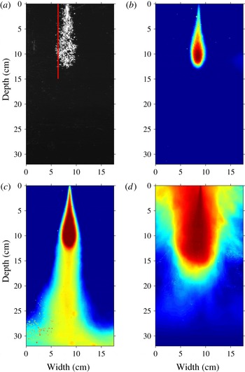
Figure 2. Illustrations of instantaneous (black and white image) and averaged (false-colour images) fountain shapes. (a) Instantaneous image in which the white regions denote light reflected from the bubbles. The air bubbles reach a maximum penetration depth of approximately 12 cm. The vertical red line defines the off-centre location of the time-series image shown in figure 4(c). (b) False-colour image in which the colour denotes a time-averaged intensity of the reflected light from the bubbles over an averaging period highlighted by the red rectangle (I) in figure 4. (c) False-colour image of the bubble fountain displayed in (b) with dyed source liquid. The averaging period corresponds to rectangle (II) in figure 4. The liquid phase of the fountain fluid continues to propagate downwards in the tank after the air bubbles have separated from the liquid. The fountains shown in panels (a–c) correspond to experiment 14 (table 1) with
 $Fr_{0}=70$
and
$Fr_{0}=70$
and
 $\unicode[STIX]{x1D6EC}=5.4$
. (d) False-colour image of a single-phase fountain (fresh water injected into a salt water solution) in which the initial buoyancy and momentum fluxes correspond to that of the bubble fountains shown in panels (a–c). The single-phase fountain reaches a maximum distance of approximately 18 cm below the nozzle and then all the fountain liquid rises to the top of the tank.
$\unicode[STIX]{x1D6EC}=5.4$
. (d) False-colour image of a single-phase fountain (fresh water injected into a salt water solution) in which the initial buoyancy and momentum fluxes correspond to that of the bubble fountains shown in panels (a–c). The single-phase fountain reaches a maximum distance of approximately 18 cm below the nozzle and then all the fountain liquid rises to the top of the tank.

Figure 3. (a) False-colour image of the averaged fountain profile recorded for experiment 14 in table 1, corresponding to the fountain shown in figure 2(a–c). In this figure, however, the image intensity has been amplified and the colour bar adjusted to visualise the cylindrical region in which the air bubbles rise after having separated from the liquid phase of the fountain fluid. (b) Cartoon summarising the experimental observations. The bubbles separate from the flow at
 $z=H_{F}$
. At this point the liquid velocity equals the bubble slip velocity,
$z=H_{F}$
. At this point the liquid velocity equals the bubble slip velocity,
 $u(H_{F})=u_{slip}$
. The liquid phase of the fountain continues to propagate as a simple jet owing to its residual momentum. The vertical coordinate,
$u(H_{F})=u_{slip}$
. The liquid phase of the fountain continues to propagate as a simple jet owing to its residual momentum. The vertical coordinate,
 $z$
, is positive downwards.
$z$
, is positive downwards.
A second imaging technique utilises time-series images, taken through the centre line of the fountain. This provides detailed information about the evolution of maximum fountain height over time (Williamson et al. Reference Williamson, Srinarayana, Armfield, McBain and Lin2008). An image of such a time series is shown in figure 4(a). The first six seconds show the penetration of air bubbles into the tank up to a maximum distance of approximately 12 cm measured from the base of the nozzle. After 6 s, the source liquid is dyed to show that the liquid phase of the fountain fluid continues to propagate downwards after the bubbles have separated from the flow. This indicates that the liquid momentum flux is not exhausted at the maximum bubble penetration depth. The two red rectangles labelled (I) and (II) define the time intervals over which the averaged fountain shapes in figure 2(b,c) have been computed.
Figure 4(b) shows a time-series image of the maximum penetration distance of a bubble fountain with an initial gas fraction of approximately
 $40\,\%$
. Although this is initially very gas rich, the mixing and dilution with ambient liquid rapidly reduces the gas fraction. The region shaded in grey is the area in which bubbles can be found. The red line marks the bottom border of the bubble region and illustrates how the instantaneous bubble penetration depth fluctuates over time, while the horizontal green line shows the time-averaged fountain depth.
$40\,\%$
. Although this is initially very gas rich, the mixing and dilution with ambient liquid rapidly reduces the gas fraction. The region shaded in grey is the area in which bubbles can be found. The red line marks the bottom border of the bubble region and illustrates how the instantaneous bubble penetration depth fluctuates over time, while the horizontal green line shows the time-averaged fountain depth.

Figure 4. (a) Time series of the vertical line through the centre of a turbulent bubble fountain, shown in false colour. For times less than 6 s, the image represents the intensity of light reflected from the bubbles. For times after 6 s, the liquid phase of the fountain fluid is dyed and may also be seen in the false-colour image. Although the bubbles only penetrate to a depth of approximately 12 cm, the liquid and hence dye continues downwards into the tank. The two red rectangles mark the time intervals over which individual frames have been averaged to extract averaged fountain shapes. These averaged fountain contours are displayed in figure 2(b,c). (b) Enlarged image of the bubble penetration depth into the tank. The bubble-laden region is shaded in grey. This image highlights the fluctuation of fountain height with time, shown as a red line. The bubble penetration depths listed in table 1 correspond to the average fountain height shown as a green horizontal line. (c) Time series of a vertical line, off centre of the fountain as indicated by the red line in figure 2(a). All lines have a similar gradient implying that the rise speed of the bubbles is
 $u_{slip}=28\pm 4~\text{cm}~\text{s}^{-1}$
. The straightness of the lines reflects the rapid adjustment of the bubbles to their terminal rise speed. The majority of the inclined lines extend to the top of the image suggesting that very few bubbles are re-entrained into the fountain.
$u_{slip}=28\pm 4~\text{cm}~\text{s}^{-1}$
. The straightness of the lines reflects the rapid adjustment of the bubbles to their terminal rise speed. The majority of the inclined lines extend to the top of the image suggesting that very few bubbles are re-entrained into the fountain.
The image in figure 4(c) shows a time series of a vertical line, away from the centre of the fountain (red line in figure 2 a). This time series identifies a series of rising bubbles, seen by the sloping lines. The majority of these lines rise to the top of the image, indicating that bubbles rise beyond the top of the fountain, and are not re-entrained.
The experimental set-up, in which we can independently control the flux of air and water through a submerged nozzle, allows us to investigate the influence of variations in the source buoyancy flux for a fixed source momentum flux. The four averaged fountain shapes displayed in false colour in figure 5 were obtained for the same source momentum flux, but the source buoyancy flux increases from panel (a) to panel (d). The liquid and the gas enter the tank through the same nozzle. Assuming that the gas and liquid have the same exit velocity from the nozzle, then an increase in either the liquid flux or the gas flux results in a larger nozzle exit velocity, as given by the relation
 $$\begin{eqnarray}u_{0}=\frac{Q_{W_{0}}+Q_{A}}{\unicode[STIX]{x03C0}b_{0}^{2}}=\frac{Q_{W_{0}}}{\unicode[STIX]{x03C0}b_{0}^{2}(1-C_{0})},\end{eqnarray}$$
where
 $Q_{W_{0}}$
and
$Q_{W_{0}}$
and
 $Q_{A}$
are the source volume fluxes of water and air, respectively and
$Q_{A}$
are the source volume fluxes of water and air, respectively and
 $C_{0}$
is the gas volume fraction inside the nozzle, given by
$C_{0}$
is the gas volume fraction inside the nozzle, given by
 $$\begin{eqnarray}C_{0}=\frac{Q_{A}}{Q_{W_{0}}+Q_{A}}.\end{eqnarray}$$
Our assumption that the nozzle exit velocities of the liquid and gas are equal in magnitude is motivated by the observation that the bubble diameters (
 $d_{B}=2{-}5~\text{mm}$
) are comparable in size to the nozzle diameters (
$d_{B}=2{-}5~\text{mm}$
) are comparable in size to the nozzle diameters (
 $d_{N}=3{-}6~\text{mm}$
).
$d_{N}=3{-}6~\text{mm}$
).
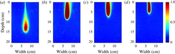
Figure 5. Four averaged fountain shapes (averaging period
 $=$
10 s) at the same constant momentum flux with different buoyancy fluxes. The source gas volume represents a fraction of (a)
$=$
10 s) at the same constant momentum flux with different buoyancy fluxes. The source gas volume represents a fraction of (a)
 $8\,\%$
(b)
$8\,\%$
(b)
 $47\,\%$
(c)
$47\,\%$
(c)
 $69\,\%$
and (d)
$69\,\%$
and (d)
 $78\,\%$
of the total volume of fluid issuing from the nozzle. The images are shown in false colour produced from the reflection of light by the bubbles in the fountain. No dye was used in the liquid phase of the fountain fluid in these experiments.
$78\,\%$
of the total volume of fluid issuing from the nozzle. The images are shown in false colour produced from the reflection of light by the bubbles in the fountain. No dye was used in the liquid phase of the fountain fluid in these experiments.
The source momentum flux is proportional to the square of the initial velocity,
 $u_{0}$
. The momentum flux is carried almost completely by the liquid phase of the fountain fluid as the density of air is three orders of magnitude smaller than the density of water. The source momentum flux can thus be written as
$u_{0}$
. The momentum flux is carried almost completely by the liquid phase of the fountain fluid as the density of air is three orders of magnitude smaller than the density of water. The source momentum flux can thus be written as
 $$\begin{eqnarray}M_{0}\approx (1-C_{0})\unicode[STIX]{x03C0}b_{0}^{2}u_{0}^{2}.\end{eqnarray}$$
Fountains with the same initial liquid flow rate and the same nozzle exit velocity have comparable initial momentum fluxes, irrespective of the air flow rate. At a constant liquid flux, the nozzle exit velocity can be kept constant by increasing the nozzle radius and simultaneously increasing the air flow rate such that
 $u_{0}$
remains unaffected. Following this procedure, we can investigate fountains with a constant source momentum flux but varying buoyancy fluxes. Figure 5 shows that increasing the initial gas volume fraction from (a) 8 % to (d) 78 % yields a height reduction of approximately 9 cm or 60 %, despite the fact that the source momentum flux remains constant. In single-phase fountains there is a decrease in fountain height when the buoyancy flux is increased for a given source momentum flux (Morton et al.
Reference Morton, Taylor and Turner1956; Turner Reference Turner1966; Hunt & Burridge Reference Hunt and Burridge2015). However, models describing the maximum penetration depth of bubbles in bubble fountains produced by a liquid jet plunging through the surface of a liquid reservoir have neglected the influence of the buoyancy flux (e.g. Clanet & Lasheras Reference Clanet and Lasheras1997). With the present experimental set-up we show that as may be anticipated from the single-phase fountain results, the source buoyancy flux can indeed have a significant effect on the maximum bubble penetration depth.
$u_{0}$
remains unaffected. Following this procedure, we can investigate fountains with a constant source momentum flux but varying buoyancy fluxes. Figure 5 shows that increasing the initial gas volume fraction from (a) 8 % to (d) 78 % yields a height reduction of approximately 9 cm or 60 %, despite the fact that the source momentum flux remains constant. In single-phase fountains there is a decrease in fountain height when the buoyancy flux is increased for a given source momentum flux (Morton et al.
Reference Morton, Taylor and Turner1956; Turner Reference Turner1966; Hunt & Burridge Reference Hunt and Burridge2015). However, models describing the maximum penetration depth of bubbles in bubble fountains produced by a liquid jet plunging through the surface of a liquid reservoir have neglected the influence of the buoyancy flux (e.g. Clanet & Lasheras Reference Clanet and Lasheras1997). With the present experimental set-up we show that as may be anticipated from the single-phase fountain results, the source buoyancy flux can indeed have a significant effect on the maximum bubble penetration depth.
2.2 Scaling of experimental results
Figure 6(a) shows the values of
 $Fr_{0}$
and
$Fr_{0}$
and
 $\unicode[STIX]{x1D6EC}$
used in each of our experiments. The colour coding indicates the measured bubble penetration depth in centimetres. Experiments reported by Turner (Reference Turner1966) and Hunt and Burridge (Reference Hunt and Burridge2015) suggest that the height of rise of single-phase fountains with
$\unicode[STIX]{x1D6EC}$
used in each of our experiments. The colour coding indicates the measured bubble penetration depth in centimetres. Experiments reported by Turner (Reference Turner1966) and Hunt and Burridge (Reference Hunt and Burridge2015) suggest that the height of rise of single-phase fountains with
 $Fr_{0}>4$
scales as
$Fr_{0}>4$
scales as
 $$\begin{eqnarray}H_{F_{single\text{-}phase}}=2.46\frac{m_{0}^{3/4}}{f_{0}^{1/2}},\end{eqnarray}$$
where
 $m_{0}^{3/4}/f_{0}^{1/2}$
is a characteristic length scale of the fountain.
$m_{0}^{3/4}/f_{0}^{1/2}$
is a characteristic length scale of the fountain.
Mingotti and Woods (Reference Mingotti and Woods2016) showed that particle-laden fountains behave similarly to single-phase fountains if
 $\unicode[STIX]{x1D6EC}_{P}=u_{fall}/u_{F}\ll 1$
, where
$\unicode[STIX]{x1D6EC}_{P}=u_{fall}/u_{F}\ll 1$
, where
 $u_{fall}$
is the terminal fall velocity of a single particle in water. For values of
$u_{fall}$
is the terminal fall velocity of a single particle in water. For values of
 $\unicode[STIX]{x1D6EC}_{P}$
greater than unity, however, the rise height of the particles decreases compared to that of a single-phase fountain. By analogy, in the present problem, we compare the terminal rise velocity of a bubble,
$\unicode[STIX]{x1D6EC}_{P}$
greater than unity, however, the rise height of the particles decreases compared to that of a single-phase fountain. By analogy, in the present problem, we compare the terminal rise velocity of a bubble,
 $u_{slip}$
, with the characteristic fountain velocity,
$u_{slip}$
, with the characteristic fountain velocity,
 $u_{F}$
. We find that
$u_{F}$
. We find that
 $u_{slip}$
has a value of
$u_{slip}$
has a value of
 $28\pm 4~\text{cm}~\text{s}^{-1}$
, in accord with published data (Clift et al.
Reference Clift, Grace and Weber2005, p. 172). This slip velocity is large compared to the characteristic fountain velocity,
$28\pm 4~\text{cm}~\text{s}^{-1}$
, in accord with published data (Clift et al.
Reference Clift, Grace and Weber2005, p. 172). This slip velocity is large compared to the characteristic fountain velocity,
 $u_{F}$
, in our experiments so that we did not access the region
$u_{F}$
, in our experiments so that we did not access the region
 $\unicode[STIX]{x1D6EC}<1$
. Our experimental data, however, confirm that the maximum bubble penetration depth decreases with
$\unicode[STIX]{x1D6EC}<1$
. Our experimental data, however, confirm that the maximum bubble penetration depth decreases with
 $\unicode[STIX]{x1D6EC}$
for
$\unicode[STIX]{x1D6EC}$
for
 $\unicode[STIX]{x1D6EC}>2$
and that these depths are smaller than the height of the analogous single-phase fountain. Indeed, figure 6(b) illustrates the maximum penetration distance of bubbles, normalised by the characteristic single-phase fountain length scale,
$\unicode[STIX]{x1D6EC}>2$
and that these depths are smaller than the height of the analogous single-phase fountain. Indeed, figure 6(b) illustrates the maximum penetration distance of bubbles, normalised by the characteristic single-phase fountain length scale,
 $m_{0}^{3/4}f_{0}^{-1/2}$
, as a function of
$m_{0}^{3/4}f_{0}^{-1/2}$
, as a function of
 $\unicode[STIX]{x1D6EC}=u_{slip}/u_{F}$
. The colour coding specifies the source Froude number for each of the 126 data points. Error bars have been omitted for clarity; these are shown in figure 9. For reference, with this scaling for the length, a classical single-phase fountain would reach a dimensionless height of 2.46. Figure 6(b) shows that the non-dimensional height decreases as
$\unicode[STIX]{x1D6EC}=u_{slip}/u_{F}$
. The colour coding specifies the source Froude number for each of the 126 data points. Error bars have been omitted for clarity; these are shown in figure 9. For reference, with this scaling for the length, a classical single-phase fountain would reach a dimensionless height of 2.46. Figure 6(b) shows that the non-dimensional height decreases as
 $\unicode[STIX]{x1D6EC}$
increases. There is also a trend in the colour coding which indicates that for a given value of
$\unicode[STIX]{x1D6EC}$
increases. There is also a trend in the colour coding which indicates that for a given value of
 $\unicode[STIX]{x1D6EC}$
, experiments with higher values of
$\unicode[STIX]{x1D6EC}$
, experiments with higher values of
 $Fr_{0}$
have systematically larger heights than experiments with lower
$Fr_{0}$
have systematically larger heights than experiments with lower
 $Fr_{0}$
(figure 6
b). In the next section, we develop a model for the bubble fountain in an attempt to understand these data.
$Fr_{0}$
(figure 6
b). In the next section, we develop a model for the bubble fountain in an attempt to understand these data.

Figure 6. (a) Illustration of the
 $Fr_{0}$
–
$Fr_{0}$
–
 $\unicode[STIX]{x1D6EC}$
-space covered by our new experiments. The colour coding specifies the bubble penetration distance in centimetres. (b) Illustration of the bubble penetration distance,
$\unicode[STIX]{x1D6EC}$
-space covered by our new experiments. The colour coding specifies the bubble penetration distance in centimetres. (b) Illustration of the bubble penetration distance,
 $H_{F}$
, normalised by the scaling for the height of a single-phase fountain,
$H_{F}$
, normalised by the scaling for the height of a single-phase fountain,
 $m_{0}^{3/4}f_{0}^{-1/2}$
, as a function of
$m_{0}^{3/4}f_{0}^{-1/2}$
, as a function of
 $\unicode[STIX]{x1D6EC}$
, the ratio of bubble slip speed and characteristic fountain velocity. The colour coding specifies
$\unicode[STIX]{x1D6EC}$
, the ratio of bubble slip speed and characteristic fountain velocity. The colour coding specifies
 $Fr_{0}$
.
$Fr_{0}$
.
3 A theoretical model
Theoretical models for turbulent single-phase fountains have been based on conservation equations for horizontally averaged momentum, buoyancy and volume fluxes (Morton et al.
Reference Morton, Taylor and Turner1956; Turner Reference Turner1966; McDougall Reference McDougall1981; Bloomfield & Kerr Reference Bloomfield and Kerr2000). We build on this approach to describe the bubble fountains produced from a co-flowing stream of air and water issuing from a submerged nozzle, as described above. On its own, the liquid stream would behave as a jet, decelerating as it entrains ambient liquid. The gas phase, however, introduces buoyancy effects, leading to a more rapid deceleration of the flow up to the point of bubble separation, which is assumed to occur when the bubble rise speed matches the downward speed of the fountain liquid. The bubbles are modelled to have a descent speed equal to the difference between the liquid velocity and their rise speed,
 $u_{B}(z)=u(z)-u_{slip}$
; we justify this simplification in appendix A in which we compare the predictions of the present simplified model with a more detailed model in which we account for the change in speed of bubbles relative to the liquid over time. Note that the rise speed of all bubbles in the size range 2 to 5 mm, which is characteristic of the present bubble fountains, is similar at approximately
$u_{B}(z)=u(z)-u_{slip}$
; we justify this simplification in appendix A in which we compare the predictions of the present simplified model with a more detailed model in which we account for the change in speed of bubbles relative to the liquid over time. Note that the rise speed of all bubbles in the size range 2 to 5 mm, which is characteristic of the present bubble fountains, is similar at approximately
 $28\pm 4~\text{cm}~\text{s}^{-1}$
(Clift et al.
Reference Clift, Grace and Weber2005, p. 172). Hence, as a first approximation, we assume there is a single rise speed.
$28\pm 4~\text{cm}~\text{s}^{-1}$
(Clift et al.
Reference Clift, Grace and Weber2005, p. 172). Hence, as a first approximation, we assume there is a single rise speed.
We introduce the variables
 $\widetilde{C}(z,r)$
,
$\widetilde{C}(z,r)$
,
 $\widetilde{u_{B}}(z,r)$
and
$\widetilde{u_{B}}(z,r)$
and
 $\widetilde{u}(z,r)$
to represent the time-averaged gas volume fraction, gas speed and liquid speed in the fountain as a function of the vertical coordinate
$\widetilde{u}(z,r)$
to represent the time-averaged gas volume fraction, gas speed and liquid speed in the fountain as a function of the vertical coordinate
 $z$
and radial coordinate
$z$
and radial coordinate
 $r$
. We denote the horizontally averaged ‘top-hat’ volume fraction,
$r$
. We denote the horizontally averaged ‘top-hat’ volume fraction,
 $C(z)$
, gas velocity
$C(z)$
, gas velocity
 $u_{B}(z)$
, liquid velocity
$u_{B}(z)$
, liquid velocity
 $u(z)$
and fountain radius
$u(z)$
and fountain radius
 $b(z)$
, in terms of the volume flux,
$b(z)$
, in terms of the volume flux,
 $Q_{W}(z)=\unicode[STIX]{x03C0}q_{W}(z)$
, gas flux,
$Q_{W}(z)=\unicode[STIX]{x03C0}q_{W}(z)$
, gas flux,
 $Q_{A}(z)=\unicode[STIX]{x03C0}q_{A}(z)$
, and momentum flux,
$Q_{A}(z)=\unicode[STIX]{x03C0}q_{A}(z)$
, and momentum flux,
 $M(z)=\unicode[STIX]{x03C0}m(z)$
in the fountain, according to the relations
$M(z)=\unicode[STIX]{x03C0}m(z)$
in the fountain, according to the relations
 $$\begin{eqnarray}\displaystyle & \displaystyle q_{A}(z)=\int _{0}^{\infty }\widetilde{C}(z,r)2r\widetilde{u_{B}}(z,r)\,\text{d}r=C(z)b(z)^{2}(u(z)-u_{slip}), & \displaystyle\end{eqnarray}$$
 $$\begin{eqnarray}\displaystyle & \displaystyle q_{W}(z)=\int _{0}^{\infty }(1-\widetilde{C}(z,r))2r\widetilde{u}(z,r)\,\text{d}r=(1-C(z))b(z)^{2}u(z), & \displaystyle\end{eqnarray}$$
 $$\begin{eqnarray}\displaystyle & \displaystyle m(z)\approx m_{W}(z)=\int _{0}^{\infty }(1-\widetilde{C}(z,r))2r\widetilde{u}(z,r)^{2}\,\text{d}r=(1-C(z))b(z)^{2}u(z)^{2}, & \displaystyle\end{eqnarray}$$
where
 $(1-C(z))$
is the liquid volume fraction. In evaluating the total momentum flux of the fountain, we should in principle account for the sum of the momentum carried by the gas and the liquid phase. However, as the density of air is three orders of magnitude smaller than the density of water, the contribution of the gas phase to the overall momentum is negligible and so in (3.3) we only account for the momentum flux of the liquid phase of the fountain fluid.
$(1-C(z))$
is the liquid volume fraction. In evaluating the total momentum flux of the fountain, we should in principle account for the sum of the momentum carried by the gas and the liquid phase. However, as the density of air is three orders of magnitude smaller than the density of water, the contribution of the gas phase to the overall momentum is negligible and so in (3.3) we only account for the momentum flux of the liquid phase of the fountain fluid.
In the model, we assume that on leaving the nozzle, the vertical bubble velocity rapidly adjusts to the value
 $u_{0}-u_{slip}$
, where the terminal bubble rise speed is
$u_{0}-u_{slip}$
, where the terminal bubble rise speed is
 $u_{slip}\approx 28~\text{cm}~\text{s}^{-1}$
. As a simplification we estimate the properties of the flow beyond this adjustment zone by assuming conservation of volume, momentum and gas flux across this zone. We denote the flow in the nozzle and downstream of the adjustment zone with the subscripts
$u_{slip}\approx 28~\text{cm}~\text{s}^{-1}$
. As a simplification we estimate the properties of the flow beyond this adjustment zone by assuming conservation of volume, momentum and gas flux across this zone. We denote the flow in the nozzle and downstream of the adjustment zone with the subscripts
 $0$
and
$0$
and
 $1$
, respectively, leading to the relations
$1$
, respectively, leading to the relations
 $$\begin{eqnarray}\displaystyle & \displaystyle (1-C_{0})b_{0}^{2}u_{0}=(1-C_{1})b_{1}^{2}u_{1}, & \displaystyle\end{eqnarray}$$
 $$\begin{eqnarray}\displaystyle & \displaystyle (1-C_{0})b_{0}^{2}u_{0}^{2}=(1-C_{1})b_{1}^{2}u_{1}^{2}, & \displaystyle\end{eqnarray}$$
 $$\begin{eqnarray}\displaystyle & \displaystyle C_{0}b_{0}^{2}u_{0}=C_{1}b_{1}^{2}(u_{1}-u_{slip}). & \displaystyle\end{eqnarray}$$
In appendix A, we show that the predictions of this model in which we assume rapid adjustment of the bubble speed on leaving the nozzle (3.4)–(3.6) are within 3 % of those of a more complete model in which we allow the bubble speed relative to the liquid speed to adjust owing to the effects of both the bubble buoyancy and the drag between the bubble and the liquid. In the main text, we now develop a model for the bubble fountain, assuming the bubble speed has value
 $u-u_{slip}$
beyond the nozzle.
$u-u_{slip}$
beyond the nozzle.
In the experiments we did not observe significant re-entrainment of bubbles back into the descending fountain flow. Indeed, figure 4(c) shows that most bubble traces extend all the way to the top of the image, indicating that after they have separated from the fountain, the bubbles rise to the surface and escape, rather then being re-entrained into the fountain core. To help understand these observations, in appendix B we calculate the trajectory of an air bubble which separates from the fountain at
 $z=H_{F}$
and
$z=H_{F}$
and
 $R(H_{F})=b_{max}$
, the outer radius of the fountain. As the bubble rises, it migrates inwards towards the fountain owing to the radial velocity field associated with the entrainment. However, the rise speed is so large that the bubbles only migrate a small radial distance prior to reaching the free surface, and hence are not re-entrained. Therefore, in the model of the fountain we assume the gas flux is independent of depth
$R(H_{F})=b_{max}$
, the outer radius of the fountain. As the bubble rises, it migrates inwards towards the fountain owing to the radial velocity field associated with the entrainment. However, the rise speed is so large that the bubbles only migrate a small radial distance prior to reaching the free surface, and hence are not re-entrained. Therefore, in the model of the fountain we assume the gas flux is independent of depth
 $$\begin{eqnarray}\frac{\text{d}}{\text{d}z}(q_{A})=0.\end{eqnarray}$$
The volume flux of water in the fountain continually increases with distance owing to the entrainment (cf. Morton et al. Reference Morton, Taylor and Turner1956)
 $$\begin{eqnarray}\frac{\text{d}}{\text{d}z}(q_{W})=2\unicode[STIX]{x1D6FC}m^{1/2}=2\unicode[STIX]{x1D6FC}b(z)u(z)\sqrt{1-C(z)}.\end{eqnarray}$$
Finally, the rate of change of momentum in the vertical direction can be expressed as
 $$\begin{eqnarray}\frac{\text{d}}{\text{d}z}(m)=-g^{\prime }(z)b(z)^{2}=-gC(z)b(z)^{2},\end{eqnarray}$$
where the minus sign is associated with the negative buoyancy force of the bubbles. It should be noted that our model applies to light fountains which initially propagate downwards. The model is strictly valid for the region in which
 $u(z)>u_{slip}$
, so that the bubbles are carried down by the fountain. As we approach the point where
$u(z)>u_{slip}$
, so that the bubbles are carried down by the fountain. As we approach the point where
 $u(z)\rightarrow u_{slip}$
, the bubbles will separate from the flow and the flux of air,
$u(z)\rightarrow u_{slip}$
, the bubbles will separate from the flow and the flux of air,
 $q_{A}$
, rapidly decreases. Since we assume the bubbles all have a similar rise speed, we can use the model to estimate the maximum depth reached by the bubbles, by finding the point where
$q_{A}$
, rapidly decreases. Since we assume the bubbles all have a similar rise speed, we can use the model to estimate the maximum depth reached by the bubbles, by finding the point where
 $u(z)=u_{slip}$
. As we approach this point, the model predicts that the radius diverges, since in the model the bubble flux is a constant (3.7); in practice, the turbulent fluctuations lead to a range of depths around this height at which the bubbles actually separate, while the liquid phase of the fountain fluid carries on downwards beyond the point of separation (figure 2
c). In this context, it is worth noting that integral models of turbulent plumes and fountains often predict a divergence of the radius as the flow approaches the maximum distance from the source (Morton et al.
Reference Morton, Taylor and Turner1956).
$u(z)=u_{slip}$
. As we approach this point, the model predicts that the radius diverges, since in the model the bubble flux is a constant (3.7); in practice, the turbulent fluctuations lead to a range of depths around this height at which the bubbles actually separate, while the liquid phase of the fountain fluid carries on downwards beyond the point of separation (figure 2
c). In this context, it is worth noting that integral models of turbulent plumes and fountains often predict a divergence of the radius as the flow approaches the maximum distance from the source (Morton et al.
Reference Morton, Taylor and Turner1956).
To proceed, it is useful to scale the momentum and water fluxes relative to their initial values, and the distance relative to the length scale of the equivalent single-phase fountain, leading to the dimensionless variables
 $$\begin{eqnarray}\hat{m}=\frac{m}{m_{0}},\quad \hat{q}=\frac{q_{w}}{q_{w_{0}}},\quad \hat{z}=z\frac{f_{0}^{1/2}}{m_{0}^{3/4}}=z\frac{(C_{0}b_{0}^{2}u_{0}g)^{1/2}}{m_{0}^{3/4}}.\end{eqnarray}$$
Equation (3.7) implies that the gas flux and therefore the buoyancy flux,
 $f_{0}$
, is a constant. The remaining two equations may be expressed in dimensionless form
$f_{0}$
, is a constant. The remaining two equations may be expressed in dimensionless form
 $$\begin{eqnarray}\frac{\text{d}\hat{m}}{\text{d}\hat{z}}=\frac{-1}{Fr_{0}}\left(\frac{1}{\displaystyle \frac{\hat{m}}{\hat{q}}-\displaystyle \frac{1}{Fr_{0}}\unicode[STIX]{x1D6EC}}\right)\end{eqnarray}$$
and
 $$\begin{eqnarray}\frac{\text{d}\hat{q}}{\text{d}\hat{z}}=Fr_{0}2\unicode[STIX]{x1D6FC}\hat{m}^{1/2}.\end{eqnarray}$$
These equations illustrate the influence on the flow of the source Froude number,
 $Fr_{0}$
, and the ratio of bubble slip speed to characteristic fountain velocity,
$Fr_{0}$
, and the ratio of bubble slip speed to characteristic fountain velocity,
 $\unicode[STIX]{x1D6EC}=u_{slip}/u_{F}$
.
$\unicode[STIX]{x1D6EC}=u_{slip}/u_{F}$
.
The only free parameter in the model is the entrainment coefficient,
 $\unicode[STIX]{x1D6FC}$
. By comparison of the model prediction with the actual fountain penetration distance for each of the 126 experiments we have run, we find that the value
$\unicode[STIX]{x1D6FC}$
. By comparison of the model prediction with the actual fountain penetration distance for each of the 126 experiments we have run, we find that the value
 $\unicode[STIX]{x1D6FC}=0.04\pm 0.004$
minimises the root-mean-square (r.m.s.) error,
$\unicode[STIX]{x1D6FC}=0.04\pm 0.004$
minimises the root-mean-square (r.m.s.) error,
 $$\begin{eqnarray}e=\sqrt{\frac{1}{126}\mathop{\sum }_{n=1}^{126}(H_{Model}(i)-H_{Exp}(i))^{2}},\end{eqnarray}$$
where
 $H_{Model}(i)$
and
$H_{Model}(i)$
and
 $H_{Exp}(i)$
are the model prediction and the experimental observation of the maximum height reached by the bubbles for experiment
$H_{Exp}(i)$
are the model prediction and the experimental observation of the maximum height reached by the bubbles for experiment
 $i$
(see figure 7
a, solid line). We have also calculated
$i$
(see figure 7
a, solid line). We have also calculated
 $$\begin{eqnarray}e_{2}=\frac{1}{126}\mathop{\sum }_{n=1}^{126}\frac{H_{Exp}(i)-H_{Model}(i)}{H_{Exp}(i)},\end{eqnarray}$$
which corresponds to the mean value of the difference between the theoretical prediction of the bubble penetration distance and the experimentally observed bubble penetration distance, as a fraction of the experimental measurement, using the data from all our experiments. In figure 7(a),
 $e_{2}$
is shown as a function of
$e_{2}$
is shown as a function of
 $\unicode[STIX]{x1D6FC}$
with the dotted line. It is seen that
$\unicode[STIX]{x1D6FC}$
with the dotted line. It is seen that
 $e_{2}=0$
when
$e_{2}=0$
when
 $\unicode[STIX]{x1D6FC}=0.04$
and that this value minimises the r.m.s. error. In figure 7(b) we illustrate the ratio of the experimentally measured bubble penetration depth and the theoretical prediction, plotted as a function of the source Froude number,
$\unicode[STIX]{x1D6FC}=0.04$
and that this value minimises the r.m.s. error. In figure 7(b) we illustrate the ratio of the experimentally measured bubble penetration depth and the theoretical prediction, plotted as a function of the source Froude number,
 $Fr_{0}$
. For our set of 126 experiments we find a standard deviation of the bubble penetration distance,
$Fr_{0}$
. For our set of 126 experiments we find a standard deviation of the bubble penetration distance,
 $\unicode[STIX]{x1D70E}_{SD}$
, of
$\unicode[STIX]{x1D70E}_{SD}$
, of
 $11.5\,\%$
and a maximum difference between the data and the model prediction of approximately 30 %. This estimate of the entrainment coefficient,
$11.5\,\%$
and a maximum difference between the data and the model prediction of approximately 30 %. This estimate of the entrainment coefficient,
 $\unicode[STIX]{x1D6FC}$
, is approximately one half of the entrainment coefficient found by Bloomfield and Kerr (Reference Bloomfield and Kerr2000) for single-phase fountains. We suggest this difference may be associated with the rising bubbles which act to suppress the formation of large-scale turbulent eddies which drive the entrainment. A similar effect was reported by Neto, Cardoso & Woods (Reference Neto, Cardoso and Woods2016).
$\unicode[STIX]{x1D6FC}$
, is approximately one half of the entrainment coefficient found by Bloomfield and Kerr (Reference Bloomfield and Kerr2000) for single-phase fountains. We suggest this difference may be associated with the rising bubbles which act to suppress the formation of large-scale turbulent eddies which drive the entrainment. A similar effect was reported by Neto, Cardoso & Woods (Reference Neto, Cardoso and Woods2016).

Figure 7. (a) The r.m.s. error (RMSE, solid line) and the error in the prediction of the mean penetration distance as a fraction of the experimentally observed value (dashed line), as a function of the entrainment coefficient
 $\unicode[STIX]{x1D6FC}$
. Both errors have their absolute minimum at
$\unicode[STIX]{x1D6FC}$
. Both errors have their absolute minimum at
 $\unicode[STIX]{x1D6FC}=0.04.$
(b) Comparison of experimental data and model prediction for the penetration depth of the bubbles,
$\unicode[STIX]{x1D6FC}=0.04.$
(b) Comparison of experimental data and model prediction for the penetration depth of the bubbles,
 $H_{Exp}/H_{Model}$
, as a function of source Froude number with a logarithmic scaling on the
$H_{Exp}/H_{Model}$
, as a function of source Froude number with a logarithmic scaling on the
 $x$
-axis (
$x$
-axis (
 $10<Fr_{0}<240$
) for an entrainment coefficient of
$10<Fr_{0}<240$
) for an entrainment coefficient of
 $\unicode[STIX]{x1D6FC}=0.04$
. The 126 data points have a mean value of 1.02 (shown as a solid horizontal line) with a standard deviation of 0.115 (shown as the two dashed horizontal lines). The maximum deviation between experimental measurement and model prediction is approximately 30 %.
$\unicode[STIX]{x1D6FC}=0.04$
. The 126 data points have a mean value of 1.02 (shown as a solid horizontal line) with a standard deviation of 0.115 (shown as the two dashed horizontal lines). The maximum deviation between experimental measurement and model prediction is approximately 30 %.
The structure of the fountain as predicted by the non-dimensional model is displayed in figure 8. The cartoon of the fountain in figure 3(b) highlights that the fountain height is measured so that the downward direction is positive. Figure 8(a–c) shows how the dimensionless momentum flux, volume flux and liquid velocity develop as one travels downwards through the fountain. All model solutions were obtained for
 $Fr_{0}=100$
and each plot contains three lines for
$Fr_{0}=100$
and each plot contains three lines for
 $\unicode[STIX]{x1D6EC}=0$
,
$\unicode[STIX]{x1D6EC}=0$
,
 $\unicode[STIX]{x1D6EC}=1$
and
$\unicode[STIX]{x1D6EC}=1$
and
 $\unicode[STIX]{x1D6EC}=3$
. Only when
$\unicode[STIX]{x1D6EC}=3$
. Only when
 $\unicode[STIX]{x1D6EC}=0$
does the momentum of the fountain fluid fall to zero as the fountain reaches its maximum depth. For
$\unicode[STIX]{x1D6EC}=0$
does the momentum of the fountain fluid fall to zero as the fountain reaches its maximum depth. For
 $\unicode[STIX]{x1D6EC}>0$
, the momentum flux is still positive at the point at which the bubbles separate from the flow.
$\unicode[STIX]{x1D6EC}>0$
, the momentum flux is still positive at the point at which the bubbles separate from the flow.

Figure 8. Variation of the non-dimensional momentum flux (a), volume flux (b), velocity (c) as a function of the distance below the source. Curves are given for the parameter values
 $\unicode[STIX]{x1D6EC}=0$
(dashed),
$\unicode[STIX]{x1D6EC}=0$
(dashed),
 $\unicode[STIX]{x1D6EC}=1$
(dotted) and
$\unicode[STIX]{x1D6EC}=1$
(dotted) and
 $\unicode[STIX]{x1D6EC}=3$
(solid), and in this case for
$\unicode[STIX]{x1D6EC}=3$
(solid), and in this case for
 $Fr_{0}=100$
.
$Fr_{0}=100$
.
Figure 9. Comparison of the theoretical model with the experimental data plotted as non-dimensional height as a function of
 $\unicode[STIX]{x1D6EC}=u_{slip}/u_{F}$
. Each plot shows four model solutions for
$\unicode[STIX]{x1D6EC}=u_{slip}/u_{F}$
. Each plot shows four model solutions for
 $Fr_{0}=10$
,
$Fr_{0}=10$
,
 $Fr_{0}=20$
,
$Fr_{0}=20$
,
 $Fr_{0}=40$
and
$Fr_{0}=40$
and
 $Fr_{0}=240$
. Panel (a) contains all data points with
$Fr_{0}=240$
. Panel (a) contains all data points with
 $40<Fr_{0}<240$
. Similarly, (b) shows the experimental data for
$40<Fr_{0}<240$
. Similarly, (b) shows the experimental data for
 $20<Fr_{0}<40$
and (c) contains the data points for
$20<Fr_{0}<40$
and (c) contains the data points for
 $12<Fr_{0}<20$
.
$12<Fr_{0}<20$
.
Figure 8(b) highlights the importance of the entrainment of ambient water into the fountain. The liquid flux rapidly increases so that the fountain fluid is soon dominated by entrained liquid rather than the initial source fluid. The liquid velocity, plotted in figure 8(c), rapidly decreases after leaving the nozzle but remains positive except in the case
 $\unicode[STIX]{x1D6EC}=0$
. Solutions of the non-dimensional model presented in (3.11) and (3.12) also allow for an investigation of the influence of
$\unicode[STIX]{x1D6EC}=0$
. Solutions of the non-dimensional model presented in (3.11) and (3.12) also allow for an investigation of the influence of
 $Fr_{0}$
and
$Fr_{0}$
and
 $\unicode[STIX]{x1D6EC}$
on the penetration depth of the bubbles. Figure 6(b) shows that the experimental measurements of non-dimensional height decrease as
$\unicode[STIX]{x1D6EC}$
on the penetration depth of the bubbles. Figure 6(b) shows that the experimental measurements of non-dimensional height decrease as
 $\unicode[STIX]{x1D6EC}$
increases and
$\unicode[STIX]{x1D6EC}$
increases and
 $Fr_{0}$
decreases. This finding is consistent with the model predictions as seen in figure 9, which illustrates the predictions of the bubble penetration distance as a function of
$Fr_{0}$
decreases. This finding is consistent with the model predictions as seen in figure 9, which illustrates the predictions of the bubble penetration distance as a function of
 $\unicode[STIX]{x1D6EC}$
for four different values of
$\unicode[STIX]{x1D6EC}$
for four different values of
 $Fr_{0}$
and compares these with our experimental measurements.
$Fr_{0}$
and compares these with our experimental measurements.
Figures 9(a)–9(c) divide the experimental data into three sets of results: (a) a high Froude number range with
 $40<Fr_{0}<240$
, (b) an intermediate range with
$40<Fr_{0}<240$
, (b) an intermediate range with
 $20<Fr_{0}<40$
and (c) all data points with
$20<Fr_{0}<40$
and (c) all data points with
 $12<Fr_{0}<20$
. The lines represent the model predictions for source Froude numbers of 10, 20, 40 and 240. Figure 9(a) shows that the majority of the data points for
$12<Fr_{0}<20$
. The lines represent the model predictions for source Froude numbers of 10, 20, 40 and 240. Figure 9(a) shows that the majority of the data points for
 $Fr_{0}>40$
lie between the model solution for
$Fr_{0}>40$
lie between the model solution for
 $Fr_{0}=40$
(blue line) and
$Fr_{0}=40$
(blue line) and
 $Fr_{0}=240$
(green line). Similarly, the majority of the data points for the intermediate and low
$Fr_{0}=240$
(green line). Similarly, the majority of the data points for the intermediate and low
 $Fr_{0}$
regimes also lie mostly between the lines delineating the model predictions for the bounding values of
$Fr_{0}$
regimes also lie mostly between the lines delineating the model predictions for the bounding values of
 $Fr_{0}$
. The error bars included in this graph reflect uncertainties in the source conditions: for our experimental system, the liquid flux is known to an accuracy of
$Fr_{0}$
. The error bars included in this graph reflect uncertainties in the source conditions: for our experimental system, the liquid flux is known to an accuracy of
 $\pm 5\,\%$
and the air flux is known to an accuracy of
$\pm 5\,\%$
and the air flux is known to an accuracy of
 $\pm 10\,\%$
.
$\pm 10\,\%$
.
4 Comparison with bubble fountains produced by plunging jets
In our experimental set-up, shown in figure 1, the nozzle is submerged under water and this allows for independent control of the air and the water flux at the source. However, turbulent bubble fountains in water are also produced when a pure downward propagating liquid jet enters the free surface of a tank of water. At the plunging point, the jet entrains air from the environment, producing a bubble fountain. A schematic of this set-up is shown in figure 11(a). In this case, the amount of entrained air is a dependent parameter, controlled by
 $d_{0},L_{J}$
and
$d_{0},L_{J}$
and
 $u_{0}$
, the diameter, length and velocity of the plunging jet respectively (Biń Reference Biń1993; Clanet & Lasheras Reference Clanet and Lasheras1997).
$u_{0}$
, the diameter, length and velocity of the plunging jet respectively (Biń Reference Biń1993; Clanet & Lasheras Reference Clanet and Lasheras1997).
Turbulent bubble fountains generated by plunging liquid jets are frequently employed in the process industry, for waste water treatment and for lake restoration (Biń Reference Biń1993). Clanet and Lasheras (Reference Clanet and Lasheras1997) have investigated such fountains and have proposed a model for the depth of penetration of bubbles entrained by such plunging water jets which takes the form
 $$\begin{eqnarray}\frac{H_{F}}{2b_{0}}=\frac{1+\tan (12.5^{\circ })}{2\tan (12.5^{\circ })}\frac{u_{0}}{u_{slip}}.\end{eqnarray}$$
This model is very different to our new model for submerged bubble fountains (presented in § 3) as it does not account for the effects of buoyancy; the maximum bubble penetration depth is independent of the air flux,
 $Q_{Air}$
. Clanet and Lasheras’ model assumes a fixed spreading angle of
$Q_{Air}$
. Clanet and Lasheras’ model assumes a fixed spreading angle of
 $12.5^{\circ }$
and a constant bubble slip velocity of
$12.5^{\circ }$
and a constant bubble slip velocity of
 $u_{slip}=22~\text{cm}~\text{s}^{-1}$
. The only free parameters in (4.1) are the jet diameter and velocity,
$u_{slip}=22~\text{cm}~\text{s}^{-1}$
. The only free parameters in (4.1) are the jet diameter and velocity,
 $d_{0}$
and
$d_{0}$
and
 $u_{0}$
. As stated in § 1, the initial momentum flux in the water jet is
$u_{0}$
. As stated in § 1, the initial momentum flux in the water jet is
 $m_{0}=b_{0}^{2}u_{0}^{2}=d_{0}^{2}u_{0}^{2}/4$
. Clanet and Lasheras’ model, given by (4.1), can therefore be written in terms of
$m_{0}=b_{0}^{2}u_{0}^{2}=d_{0}^{2}u_{0}^{2}/4$
. Clanet and Lasheras’ model, given by (4.1), can therefore be written in terms of
 $m_{0}$
according to the relation
$m_{0}$
according to the relation
 $$\begin{eqnarray}H_{F}\approx 25b_{0}u_{0}=25m_{0}^{1/2}.\end{eqnarray}$$
This expression, which does not account for the effects of the gas phase, corresponds to the evolution of a simple single-phase jet, decelerating as it entrains ambient water. The equivalent entrainment coefficient would be 0.07. A simple decelerating jet would propagate over very long distances. Clanet and Lasheras, however, define the point at which the fountain liquid velocity matches the bubble rise speed as the point of maximum bubble penetration depth,
 $u(z_{max})=u_{slip}$
.
$u(z_{max})=u_{slip}$
.
Clanet and Lasheras’ model, expressed in simplified form in (4.2), depends only on the initial momentum flux. No account of the bubble buoyancy on the dynamics of the fountain is included. With our new experimental set-up with a submerged nozzle, however, we were able to vary the buoyancy flux for a given momentum flux. In figure 5, we clearly show that the maximum bubble penetration depth decreases for larger buoyancy fluxes at a constant initial momentum flux. We conducted this investigation for four initial momentum fluxes. For each momentum flux we produced fountains with four different gas fractions ranging from
 $10$
to
$10$
to
 $80\,\%$
, resulting in a total of 16 data points. The reduction in fountain height with increasing gas volume fraction is displayed in figure 10. The sloped lines describe the best linear fit through the bubble penetration distance measurements for a fixed source momentum flux. Clanet and Lasheras’ model (4.1) does not depend on the gas fraction and therefore predicts a constant bubble penetration depth for a given momentum flux. This prediction is plotted as a short horizontal line at the intersection of the best-fit line and the model prediction. This point of intersection serves as a rough approximation for the gas flux entrained by the plunging jet experiments of Clanet and Lasheras (Reference Clanet and Lasheras1997).
$80\,\%$
, resulting in a total of 16 data points. The reduction in fountain height with increasing gas volume fraction is displayed in figure 10. The sloped lines describe the best linear fit through the bubble penetration distance measurements for a fixed source momentum flux. Clanet and Lasheras’ model (4.1) does not depend on the gas fraction and therefore predicts a constant bubble penetration depth for a given momentum flux. This prediction is plotted as a short horizontal line at the intersection of the best-fit line and the model prediction. This point of intersection serves as a rough approximation for the gas flux entrained by the plunging jet experiments of Clanet and Lasheras (Reference Clanet and Lasheras1997).
Figure 10. Variation of the maximum bubble penetration depth for fountains with the same initial momentum flux. The source momentum flux was kept constant by fixing the liquid volume flux and adjusting nozzle diameter and air flux such that the source velocity,
 $u_{0}$
, remains unchanged. Each of the sloped lines is a linear best fit through four fountain height measurements at a constant momentum flux,
$u_{0}$
, remains unchanged. Each of the sloped lines is a linear best fit through four fountain height measurements at a constant momentum flux,
 $m_{0}=q_{W_{0}}u_{0}$
, but varying source gas fluxes. Increasing the source gas flux at a fixed momentum flux yields a reduction in bubble penetration depth. The dashed line (third line from the top) corresponds to the averaged fountain shapes shown in figure 5. The horizontal lines correspond to the height predicted by the model presented by Clanet and Lasheras (Reference Clanet and Lasheras1997).
$m_{0}=q_{W_{0}}u_{0}$
, but varying source gas fluxes. Increasing the source gas flux at a fixed momentum flux yields a reduction in bubble penetration depth. The dashed line (third line from the top) corresponds to the averaged fountain shapes shown in figure 5. The horizontal lines correspond to the height predicted by the model presented by Clanet and Lasheras (Reference Clanet and Lasheras1997).
Even though Clanet and Lasheras’ model neglects the influence of buoyancy on the maximum bubble penetration depth, their predictions are in very good agreement with their experimental data. A resolution of this seems to be that the model of Clanet and Lasheras implies an entrainment coefficient of approximately 0.07, which is much larger than we have determined for our model (§ 3). The enhanced entrainment predicts a faster deceleration of the fountain and this compensates for the lack of the negative buoyancy force associated with the bubbles, which also acts to decelerate the fountain.
We can re-interpret the experimental data on the penetration depth of the bubble fountains produced by a plunging jet provided by Clanet and Lasheras (Reference Clanet and Lasheras1997) using our new theoretical model. The liquid and momentum fluxes at the source are known as well as the measured bubble penetration depth. For each data point we can therefore find a gas flux so that the maximum bubble penetration distance predicted by our new model corresponds to the published fountain height measurement. Figure 11 illustrates the prediction of the ratio of the flux of entrained air as a fraction of the source liquid flow rate,
 $Q_{A}/Q_{W_{0}}$
, as a function of the dimensionless parameter
$Q_{A}/Q_{W_{0}}$
, as a function of the dimensionless parameter
 $\unicode[STIX]{x1D6FA}=u_{0}^{2}/(gd_{0})$
, where
$\unicode[STIX]{x1D6FA}=u_{0}^{2}/(gd_{0})$
, where
 $d_{0}$
is the nozzle diameter. Although there are no data on the actual gas flux in these specific plunging jets, we can nevertheless check if our predictions are consistent with empirical laws which have been published for the rate of entrainment of air into similar plunging jets. For example, we compare our results with two empirical relationships (Van de Donk (Reference Van de Donk1981), dashed line, and Ohkawa et al. (Reference Ohkawa, Kusabiraki, Kawai, Sakai and Endoh1986), solid line) between the bubble penetration distance and the ratio of gas flux to liquid flux which are based on experimental measurements (Biń Reference Biń1993). Our estimates of the gas flux entrained into the plunging liquid jets reported by Clanet and Lasheras (Reference Clanet and Lasheras1997) are consistent with these empirical relations; indeed the majority of our predictions fall between those of the two empirical models. This statement holds true for both the model presented in § 3 and for the model presented in appendix A which allows for an adjustment in bubble velocity. The predictions for the flux of entrained air of the two models agree to within 3 %. We do note that some caution is required since there is a non-negligible difference between the two empirical models plotted in figure 11.
$d_{0}$
is the nozzle diameter. Although there are no data on the actual gas flux in these specific plunging jets, we can nevertheless check if our predictions are consistent with empirical laws which have been published for the rate of entrainment of air into similar plunging jets. For example, we compare our results with two empirical relationships (Van de Donk (Reference Van de Donk1981), dashed line, and Ohkawa et al. (Reference Ohkawa, Kusabiraki, Kawai, Sakai and Endoh1986), solid line) between the bubble penetration distance and the ratio of gas flux to liquid flux which are based on experimental measurements (Biń Reference Biń1993). Our estimates of the gas flux entrained into the plunging liquid jets reported by Clanet and Lasheras (Reference Clanet and Lasheras1997) are consistent with these empirical relations; indeed the majority of our predictions fall between those of the two empirical models. This statement holds true for both the model presented in § 3 and for the model presented in appendix A which allows for an adjustment in bubble velocity. The predictions for the flux of entrained air of the two models agree to within 3 %. We do note that some caution is required since there is a non-negligible difference between the two empirical models plotted in figure 11.
Figure 11. (a) Schematic of a bubble fountain generated by a liquid jet plunging through a liquid surface. The curved arrows represent the air entrainment at the plunging point. For bubble fountains in water this air flux,
 $Q_{A}$
, is fixed for a given jet diameter,
$Q_{A}$
, is fixed for a given jet diameter,
 $d_{0}$
, jet length,
$d_{0}$
, jet length,
 $L_{J}$
, and jet velocity,
$L_{J}$
, and jet velocity,
 $u_{0}$
. (b) The new theoretical model was applied to existing experimental data (Clanet & Lasheras Reference Clanet and Lasheras1997) to calculate the amount of air entrained by plunging liquid jets based on the source momentum flux of the water jet and the maximum penetration depth of the resulting bubble fountain. The ratio of entrained gas to initial liquid flux,
$u_{0}$
. (b) The new theoretical model was applied to existing experimental data (Clanet & Lasheras Reference Clanet and Lasheras1997) to calculate the amount of air entrained by plunging liquid jets based on the source momentum flux of the water jet and the maximum penetration depth of the resulting bubble fountain. The ratio of entrained gas to initial liquid flux,
 $Q_{A}/Q_{W_{0}}$
, for these data points, shown as black squares, is plotted as a function of
$Q_{A}/Q_{W_{0}}$
, for these data points, shown as black squares, is plotted as a function of
 $\unicode[STIX]{x1D6FA}=u_{0}^{2}/(gd_{0})$
. The data points are compared against empirical fits (Van de Donk Reference Van de Donk1981; Ohkawa et al.
Reference Ohkawa, Kusabiraki, Kawai, Sakai and Endoh1986) to show that the new model can be used to calculate a first approximation of the entrained gas flux for plunging water jets.
$\unicode[STIX]{x1D6FA}=u_{0}^{2}/(gd_{0})$
. The data points are compared against empirical fits (Van de Donk Reference Van de Donk1981; Ohkawa et al.
Reference Ohkawa, Kusabiraki, Kawai, Sakai and Endoh1986) to show that the new model can be used to calculate a first approximation of the entrained gas flux for plunging water jets.
5 Summary
We have studied the dynamics of turbulent bubble fountains in fresh water with a series of new experiments complemented by a theoretical model based on conservation of the volume, momentum and buoyancy fluxes. We show that the penetration depth of the bubble fountains is controlled by the source Froude number,
 $Fr_{0}$
, as well as
$Fr_{0}$
, as well as
 $\unicode[STIX]{x1D6EC}$
, the ratio of bubble rise speed to characteristic fountain velocity. The predictions of the model are consistent with our new experimental measurements of the penetration distance of the bubbles in the case of an entrainment coefficient
$\unicode[STIX]{x1D6EC}$
, the ratio of bubble rise speed to characteristic fountain velocity. The predictions of the model are consistent with our new experimental measurements of the penetration distance of the bubbles in the case of an entrainment coefficient
 $\unicode[STIX]{x1D6FC}=0.04\pm 0.004$
. Our model assumes that there is little re-entrainment of rising gas bubbles and this is motivated by the observation that the bubble rise speed is large compared to the entrainment velocity. We find that the bubbles separate from the fountain at the point where the liquid velocity matches the bubble rise speed and the liquid phase of the fountain fluid continues to travel downwards owing to its residual momentum. We further show that the new theoretical model can be applied to estimate the volume of air entrained by plunging water jets based on the observed bubble penetration distance. In future work we plan to explore a generalisation of the modelling in the case that there is a range of bubble sizes and hence bubble rise velocities, as well as in the case that the ambient liquid lies in a confined space so that filling-box effects need to be considered (cf. Baines and Turner Reference Baines and Turner1969).
$\unicode[STIX]{x1D6FC}=0.04\pm 0.004$
. Our model assumes that there is little re-entrainment of rising gas bubbles and this is motivated by the observation that the bubble rise speed is large compared to the entrainment velocity. We find that the bubbles separate from the fountain at the point where the liquid velocity matches the bubble rise speed and the liquid phase of the fountain fluid continues to travel downwards owing to its residual momentum. We further show that the new theoretical model can be applied to estimate the volume of air entrained by plunging water jets based on the observed bubble penetration distance. In future work we plan to explore a generalisation of the modelling in the case that there is a range of bubble sizes and hence bubble rise velocities, as well as in the case that the ambient liquid lies in a confined space so that filling-box effects need to be considered (cf. Baines and Turner Reference Baines and Turner1969).
Acknowledgements
This work was funded through the BP Institute, a Benefactors’ Scholarship from St John’s College, Cambridge, the German Academic Scholarship Foundation (Studienstiftung des deutschen Volkes) and an EPSRC Industrial CASE Award.
Appendix A. Adjustment of the bubble velocity inside the fountain
The theoretical model presented in § 3 assumes that on exiting the nozzle and adjusting, the downward velocity of the gas phase,
 $u_{B}$
, differs from the downward liquid velocity,
$u_{B}$
, differs from the downward liquid velocity,
 $u$
, by a constant equal to the bubble rise speed,
$u$
, by a constant equal to the bubble rise speed,
 $\unicode[STIX]{x0394}u=u-u_{B}=u_{slip}=0.28~\text{m}~\text{s}^{-1}$
(see (3.1)). Inside the nozzle, however, we assume that the velocities of the gas and the liquid phase are equal in magnitude since the gas bubbles are observed to be of comparable radius to the radius of the nozzle (see (2.1)). Our assumption that the gas bubbles rapidly decelerate until attaining the constant slip velocity,
$\unicode[STIX]{x0394}u=u-u_{B}=u_{slip}=0.28~\text{m}~\text{s}^{-1}$
(see (3.1)). Inside the nozzle, however, we assume that the velocities of the gas and the liquid phase are equal in magnitude since the gas bubbles are observed to be of comparable radius to the radius of the nozzle (see (2.1)). Our assumption that the gas bubbles rapidly decelerate until attaining the constant slip velocity,
 $\unicode[STIX]{x0394}u=u_{slip}$
, is a simplification since the adjustment in bubble speed occurs over a finite adjustment length. We now show that provided this adjustment length is short compared to the length scale over which the momentum flux evolves, then this simplification does not have a large effect on the prediction of the maximum penetration distance of the bubbles in the fountain. The main effect of the bubble slip velocity on the motion of the fountain relates to its impact on the buoyancy force. Provided that the length scale over which the bubbles adjust to the terminal speed relative to the liquid is short compared to the length scale over which the buoyancy forces are important, then the buoyancy and momentum flux of the jet beyond the transition region is similar to that at the source. In this appendix, we explore this simplification in some detail. To this end, we introduce a further equation which accounts for the deceleration of the gas phase relative to the liquid
$\unicode[STIX]{x0394}u=u_{slip}$
, is a simplification since the adjustment in bubble speed occurs over a finite adjustment length. We now show that provided this adjustment length is short compared to the length scale over which the momentum flux evolves, then this simplification does not have a large effect on the prediction of the maximum penetration distance of the bubbles in the fountain. The main effect of the bubble slip velocity on the motion of the fountain relates to its impact on the buoyancy force. Provided that the length scale over which the bubbles adjust to the terminal speed relative to the liquid is short compared to the length scale over which the buoyancy forces are important, then the buoyancy and momentum flux of the jet beyond the transition region is similar to that at the source. In this appendix, we explore this simplification in some detail. To this end, we introduce a further equation which accounts for the deceleration of the gas phase relative to the liquid
 $$\begin{eqnarray}\left(\unicode[STIX]{x1D70C}_{air}+\frac{1}{2}\unicode[STIX]{x1D70C}_{w}\right)\frac{4}{3}\unicode[STIX]{x03C0}R_{B}^{3}\frac{\text{d}}{\text{d}t}(\unicode[STIX]{x0394}u)=\frac{4}{3}\unicode[STIX]{x03C0}R_{B}^{3}g(\unicode[STIX]{x1D70C}_{w}-\unicode[STIX]{x1D70C}_{air})-C_{D}(Re_{B})\unicode[STIX]{x03C0}R_{B}^{2}\frac{1}{2}\unicode[STIX]{x1D70C}_{w}\unicode[STIX]{x0394}u^{2}.\end{eqnarray}$$
The term in parentheses on the left-hand side accounts for the added mass effect owing to the displacement of ambient liquid around the bubble. The first term on the right-hand side is the buoyancy force experienced by a single bubble. The second term on the right-hand side provides a representation of the total drag on the bubble, where
 $C_{D}(Re_{B})$
is the drag coefficient,
$C_{D}(Re_{B})$
is the drag coefficient,
 $R_{B}$
is the bubble radius and
$R_{B}$
is the bubble radius and
 $(\text{d}/\text{d}t)(\unicode[STIX]{x0394}u)$
describes the bubble deceleration relative to the liquid velocity in the vertical direction. The bubble Reynolds number is defined in terms of the liquid density,
$(\text{d}/\text{d}t)(\unicode[STIX]{x0394}u)$
describes the bubble deceleration relative to the liquid velocity in the vertical direction. The bubble Reynolds number is defined in terms of the liquid density,
 $\unicode[STIX]{x1D70C}_{w}$
, the relative speed of the fluid and bubbles,
$\unicode[STIX]{x1D70C}_{w}$
, the relative speed of the fluid and bubbles,
 $\unicode[STIX]{x0394}u$
, the fluid viscosity,
$\unicode[STIX]{x0394}u$
, the fluid viscosity,
 $\unicode[STIX]{x1D707}_{w}$
, and the bubble diameter,
$\unicode[STIX]{x1D707}_{w}$
, and the bubble diameter,
 $d_{B}$
, according to the relation
$d_{B}$
, according to the relation
 $$\begin{eqnarray}Re_{B}=\frac{\unicode[STIX]{x1D70C}_{w}\unicode[STIX]{x0394}ud_{B}}{\unicode[STIX]{x1D707}_{w}}.\end{eqnarray}$$
The drag coefficient,
 $C_{D}$
, is a function of the bubble Reynolds number and experimental measurements (Turton & Levenspiel Reference Turton and Levenspiel1986) have been approximated by the empirical expression
$C_{D}$
, is a function of the bubble Reynolds number and experimental measurements (Turton & Levenspiel Reference Turton and Levenspiel1986) have been approximated by the empirical expression
 $$\begin{eqnarray}C_{D}(Re_{B})=\frac{24}{Re_{B}}(1+0.173Re_{B}^{0.657})+\frac{0.413}{1+16\,300Re_{B}^{-1.09}}.\end{eqnarray}$$
The time derivative in (A 1) can be transformed into a spatial derivative using the chain rule
 $$\begin{eqnarray}\frac{\text{d}}{\text{d}t}(\unicode[STIX]{x0394}u)=u_{B}\frac{\text{d}}{\text{d}z_{B}}(\unicode[STIX]{x0394}u)\approx 2g^{\prime }-C_{D}(Re_{B})\frac{3}{4R_{B}}\unicode[STIX]{x0394}u^{2},\end{eqnarray}$$
where
 $z_{B}$
is the position of the bubble relative to the nozzle, and the vertical velocity of the bubble,
$z_{B}$
is the position of the bubble relative to the nozzle, and the vertical velocity of the bubble,
 $u_{B}(z)$
, has an initial value of
$u_{B}(z)$
, has an initial value of
 $u_{B}(0)=u_{0}$
and adjusts towards the value
$u_{B}(0)=u_{0}$
and adjusts towards the value
 $u-u_{slip}$
when the bubble has travelled a distance of order
$u-u_{slip}$
when the bubble has travelled a distance of order
 $Z_{B}^{\ast }$
from the nozzle. We can rewrite (A 4) in the form
$Z_{B}^{\ast }$
from the nozzle. We can rewrite (A 4) in the form
 $$\begin{eqnarray}\frac{\text{d}}{\text{d}z_{B}}(u)-\frac{\text{d}}{\text{d}z_{B}}(u_{B})\approx \frac{2g^{\prime }}{u_{B}}-C_{D}(Re_{B})\frac{3}{4R_{B}u_{B}}\unicode[STIX]{x0394}u^{2}.\end{eqnarray}$$
By combining this equation with the equations for conservation of mass, momentum and buoyancy, we can find the variation of the velocity, buoyancy and radius of the fountain with distance from the source. Also the expression for the gas flux, equation (3.1), is generalised to the form
 $$\begin{eqnarray}q_{A}(z)=\int _{0}^{\infty }\widetilde{C}(z,r)2r\widetilde{u_{B}}(z,r)\,\text{d}r=C(z)b(z)^{2}u_{B}.\end{eqnarray}$$

Figure 12. (a) Illustration of the evolution of the three terms of (A 5) as a function of normalised distance from the source. Initially, the bubble decelerates owing to its buoyancy, but in steady state, the buoyancy is balanced by the turbulent drag. (b) Evolution of the liquid and bubble velocity plotted as a function of non-dimensional distance from the source. The dashed blue and red lines correspond to the predictions of the simplified model presented in § 3 of the main body of this paper. The solid blue line illustrates a gradual deceleration of the bubble compared to the liquid (black line) as predicted by the model which accounts for the evolution of the bubble velocity relative to the liquid as presented in this appendix. (c) Plot of Reynolds number as a function of the dimensionless distance from the source as predicted by the model of appendix A. (d) Plot of normalised liquid velocity (solid line) and the difference between liquid and bubble velocity (dashed line) as a function of fountain height as predicted by the model of appendix A. (e) Evolution of momentum flux and (f) liquid flux as a function of distance from the source. The red line corresponds to the model in § 3 of the main paper and the black line shows the prediction of the model presented in appendix A. For all panels, the source conditions correspond to experiment 1 in table 1 (
 $Fr_{0}=86$
).
$Fr_{0}=86$
).

Figure 13. Comparison of the model predictions of the maximum bubble penetration depth as predicted by the two models:
 $H_{u_{B}}$
corresponds to the penetration depth predicted by the model of appendix A, which allows the bubble speed relative to the liquid to vary with position, while
$H_{u_{B}}$
corresponds to the penetration depth predicted by the model of appendix A, which allows the bubble speed relative to the liquid to vary with position, while
 $H_{u-u_{slip}}$
corresponds to the model presented in § 3 of the main paper, in which the bubble is assumed to have a constant slip velocity relative to the liquid. In the figure, the ratio of
$H_{u-u_{slip}}$
corresponds to the model presented in § 3 of the main paper, in which the bubble is assumed to have a constant slip velocity relative to the liquid. In the figure, the ratio of
 $H_{u_{B}}$
to
$H_{u_{B}}$
to
 $H_{u-u_{slip}}$
is shown as a function of the source Froude number for the source conditions of all 126 experiments. The difference between the model predictions is somewhat larger for lower Froude numbers, but is always less than
$H_{u-u_{slip}}$
is shown as a function of the source Froude number for the source conditions of all 126 experiments. The difference between the model predictions is somewhat larger for lower Froude numbers, but is always less than
 $3\,\%$
.
$3\,\%$
.
If we combine (A 5) with equations (3.2)–(3.9) we can then solve for the motion of the bubble fountain. In figure 12 we illustrate a series of predictions of the model presented in this appendix (solid lines) and we compare these with the predictions of the simplified model proposed in § 3 of the main text (dashed lines). In figure 12(a), we show the prediction of the magnitude of the buoyancy force acting on a bubble (black line), the drag force acting on a bubble (red line) and the acceleration of the bubble (blue line). The buoyancy force is matched by the sum of the drag and the acceleration of the bubble (A 1). Initially, on leaving the nozzle, the dominant balance is between the buoyancy and the acceleration of the bubble. However, as the bubble speed adjusts in the first 10–20 % of the total fountain height, the force balance becomes dominated by a balance between the buoyancy force and the drag and subsequently the bubble moves with the high Reynolds number near-constant slip velocity relative to the liquid. In panel (b), we illustrate the model prediction of the velocity of the fountain liquid (red and black) and the bubbles (blue) as a function of depth. It is seen that the more complete model presented in this appendix (solid blue line) leads to a delay in the deceleration of the bubbles compared to the approximate model of the main text (dashed blue line). However, there is little difference in the predictions of the speed of the liquid in the fountain. Panel (c) illustrates the rapid increase in the bubble Reynolds number as the bubbles adjust to their slip speed in the upper 20 % of the fountain. Panel (d) clarifies the evolution of the bubble slip speed (dashed line) with position in the jet, as given by a local balance between the buoyancy force and the drag, as well as the mean speed of the liquid (solid line), while panels (e,f) illustrate that the momentum flux and volume flux of the fountain as predicted by the model presented in this appendix is indistinguishable from the prediction of the simplified model given in the main text.
In figure 13 we compare the predictions of the bubble penetration depth as given by the model in this appendix (labelled
 $H_{u_{B}}$
) and the simplified model of § 3 in the main text (
$H_{u_{B}}$
) and the simplified model of § 3 in the main text (
 $H_{u-u_{slip}}$
). The data are plotted as a function of the source Froude number for the conditions pertaining in all 126 experiments reported herein. The difference between the predictions of the two models is less than
$H_{u-u_{slip}}$
). The data are plotted as a function of the source Froude number for the conditions pertaining in all 126 experiments reported herein. The difference between the predictions of the two models is less than
 $3\,\%$
.
$3\,\%$
.
Figure 13 suggests that for the parameter space covered by our experiments, the model predictions for maximum bubble penetration depth are insensitive to the choice of initial gas phase velocity in the range from
 $\unicode[STIX]{x0394}u=0$
to
$\unicode[STIX]{x0394}u=0$
to
 $\unicode[STIX]{x0394}u=u_{slip}=0.28~\text{m}~\text{s}^{-1}$
. This results from the fact that the length over which the bubbles adjust to the liquid speed minus the high Reynolds number slip velocity is short compared to the length scale over which the buoyancy flux begins to influence the momentum flux of the fountain. Figure 8 illustrates the variation of the momentum flux, volume flux and velocity as a function of depth. The figure illustrates that on exiting the nozzle, the liquid velocity rapidly decreases, whereas the momentum flux in the vertical direction remains constant for the first 20 % of the distance travelled by the fountain. In the parameter regime covered by the present experiments, the momentum flux of the fountain only begins to evolve once the bubbles have adjusted to a downward velocity corresponding to
$\unicode[STIX]{x0394}u=u_{slip}=0.28~\text{m}~\text{s}^{-1}$
. This results from the fact that the length over which the bubbles adjust to the liquid speed minus the high Reynolds number slip velocity is short compared to the length scale over which the buoyancy flux begins to influence the momentum flux of the fountain. Figure 8 illustrates the variation of the momentum flux, volume flux and velocity as a function of depth. The figure illustrates that on exiting the nozzle, the liquid velocity rapidly decreases, whereas the momentum flux in the vertical direction remains constant for the first 20 % of the distance travelled by the fountain. In the parameter regime covered by the present experiments, the momentum flux of the fountain only begins to evolve once the bubbles have adjusted to a downward velocity corresponding to
 $u_{B}=u-u_{slip}$
. We can show this more rigorously by comparing the length scales over which changes in bubble velocity, volume flux and momentum flux occur in dimensionless form. To identify scalings, some analysis of the governing equations is helpful. The right-hand side of (A 5) can be rewritten in terms of its characteristic roots, which are
$u_{B}=u-u_{slip}$
. We can show this more rigorously by comparing the length scales over which changes in bubble velocity, volume flux and momentum flux occur in dimensionless form. To identify scalings, some analysis of the governing equations is helpful. The right-hand side of (A 5) can be rewritten in terms of its characteristic roots, which are
 $$\begin{eqnarray}\unicode[STIX]{x0394}u_{1,2}^{\ast }=\pm \sqrt{\frac{8g^{\prime }R_{B}}{3C_{D}(Re_{B})}}\approx \pm \sqrt{\frac{8gR_{B}}{3C_{D}(Re_{B})}}.\end{eqnarray}$$
Since the density of air is very small compared to the density of water the effective buoyancy,
 $g^{\prime }$
, is approximately equal to the acceleration due to gravity,
$g^{\prime }$
, is approximately equal to the acceleration due to gravity,
 $g^{\prime }\approx g$
. Using these characteristic roots, equation (A 4) can be rewritten as
$g^{\prime }\approx g$
. Using these characteristic roots, equation (A 4) can be rewritten as
 $$\begin{eqnarray}(u-\unicode[STIX]{x0394}u)\frac{\text{d}}{\text{d}z_{B}}(\unicode[STIX]{x0394}u)\approx \unicode[STIX]{x1D6FE}(\unicode[STIX]{x0394}u-\unicode[STIX]{x0394}u_{1}^{\ast })(\unicode[STIX]{x0394}u-\unicode[STIX]{x0394}u_{2}^{\ast }),\end{eqnarray}$$
where
 $\unicode[STIX]{x1D6FE}=3C_{D}(Re_{B})/4R_{B}$
. In our experiments the average bubble radius is approximately 1.5 mm, so that
$\unicode[STIX]{x1D6FE}=3C_{D}(Re_{B})/4R_{B}$
. In our experiments the average bubble radius is approximately 1.5 mm, so that
 $\unicode[STIX]{x1D6FE}\approx 500C_{D}(Re_{B})[1/m]$
. The remaining two equations are
$\unicode[STIX]{x1D6FE}\approx 500C_{D}(Re_{B})[1/m]$
. The remaining two equations are
 $$\begin{eqnarray}\frac{\text{d}(q_{W})}{\text{d}z}=\frac{\text{d}}{\text{d}z}((1-C(z))b(z)^{2}u(z))=2\unicode[STIX]{x1D6FC}m^{1/2}=2\unicode[STIX]{x1D6FC}b(z)u(z)\sqrt{1-C(z)}\end{eqnarray}$$
and
 $$\begin{eqnarray}\frac{\text{d}(m)}{\text{d}z}=\frac{\text{d}}{\text{d}z}((1-C(z))b(z)^{2}u(z)^{2})=-g^{\prime }(z)b(z)^{2}=-\frac{f_{0}}{u_{B}}.\end{eqnarray}$$
Scaling the drag coefficient with the value at high Reynolds numbers,
 $C_{D_{\infty }}$
, we can define a normalised drag coefficient,
$C_{D_{\infty }}$
, we can define a normalised drag coefficient,
 $\hat{C_{D}}=C_{D}(Re_{B})/C_{D_{\infty }}$
for each value of
$\hat{C_{D}}=C_{D}(Re_{B})/C_{D_{\infty }}$
for each value of
 $Re_{B}$
. We proceed by scaling the vertical coordinate,
$Re_{B}$
. We proceed by scaling the vertical coordinate,
 $z$
by
$z$
by
 $\unicode[STIX]{x1D6E4}=3C_{D_{\infty }}/(4R_{B})\approx 250[1/m]$
so that
$\unicode[STIX]{x1D6E4}=3C_{D_{\infty }}/(4R_{B})\approx 250[1/m]$
so that
 $\hat{z}=z\unicode[STIX]{x1D6E4}$
. The remaining dimensionless variables may be defined as
$\hat{z}=z\unicode[STIX]{x1D6E4}$
. The remaining dimensionless variables may be defined as
 $$\begin{eqnarray}\hat{u} =\frac{u}{u_{slip}};\quad \hat{\unicode[STIX]{x0394}u}=\frac{\unicode[STIX]{x0394}u}{u_{slip}};\quad \hat{\hat{u} }=\frac{u}{u_{0}};\quad V=\frac{u_{0}}{u_{slip}};\quad \hat{u} =V\hat{\hat{u} };\quad \hat{b}=\frac{b}{b_{0}}.\end{eqnarray}$$
It is important to note that the right-hand side of (A 7) can be expressed in the form
 $$\begin{eqnarray}u_{s}(Re_{B})=\sqrt{\frac{8gR_{B}}{3C_{D}(Re_{B})}}=\sqrt{\frac{1}{\hat{C_{D}}}}u_{slip},\end{eqnarray}$$
where the constant high Reynolds number bubble slip speed is
 $$\begin{eqnarray}u_{slip}=\sqrt{\frac{8gR_{B}}{3C_{D_{\infty }}}}.\end{eqnarray}$$
For our average observed bubble radius of 1.5 mm and a drag coefficient at high Reynolds numbers of
 $C_{D_{\infty }}\approx 0.5$
(Schlichting Reference Schlichting1979; Turton & Levenspiel Reference Turton and Levenspiel1986) we find
$C_{D_{\infty }}\approx 0.5$
(Schlichting Reference Schlichting1979; Turton & Levenspiel Reference Turton and Levenspiel1986) we find
 $u_{slip}=0.28~\text{m}~\text{s}^{-1}$
. With these scalings, equations (A 8)–(A 10) can be written in dimensionless form as
$u_{slip}=0.28~\text{m}~\text{s}^{-1}$
. With these scalings, equations (A 8)–(A 10) can be written in dimensionless form as
 $$\begin{eqnarray}\displaystyle & \displaystyle \left(\hat{\hat{u} }-\frac{\hat{\unicode[STIX]{x0394}u}}{V}\right)\frac{\text{d}}{\text{d}\hat{z_{B}}}(\hat{\unicode[STIX]{x0394}u})\approx \frac{1}{V}\left(\hat{\unicode[STIX]{x0394}u}-\frac{1}{\sqrt{\hat{C_{D}}}}\right)\left(\hat{\unicode[STIX]{x0394}u}+\frac{1}{\sqrt{\hat{C_{D}}}}\right), & \displaystyle\end{eqnarray}$$
 $$\begin{eqnarray}\displaystyle & \displaystyle \frac{\text{d}}{\text{d}\hat{z}}((1-C)\hat{b}^{2}\hat{\hat{u} })=\frac{2\unicode[STIX]{x1D6FC}}{b_{0}\unicode[STIX]{x1D6E4}}\hat{b}\hat{\hat{u} }\sqrt{1-C}, & \displaystyle\end{eqnarray}$$
 $$\begin{eqnarray}\displaystyle & \displaystyle \left(\hat{\hat{u} }-\frac{\hat{\unicode[STIX]{x0394}u}}{V}\right)\frac{\text{d}}{\text{d}\hat{z}}((1-C)\hat{b}^{2}\hat{\hat{u} }^{2})=-\frac{f_{0}}{V^{3}u_{slip}^{3}\unicode[STIX]{x1D6E4}b_{0}^{2}}. & \displaystyle\end{eqnarray}$$
In this form, the non-dimensional pre-factors on the right-hand side of each equation allow for a comparison of how quickly the bubble velocity, liquid flux and momentum flux adjust in the fountain. Equation (A 14) suggests that with
 $V\gg 1$
, the length scale for the adjustment of the bubble speed is given by
$V\gg 1$
, the length scale for the adjustment of the bubble speed is given by
 $Z_{Bubble}^{\ast }=V$
. The corresponding length scale for the adjustment of the momentum flux, as given by (A 16), is
$Z_{Bubble}^{\ast }=V$
. The corresponding length scale for the adjustment of the momentum flux, as given by (A 16), is
 $Z_{mmt}^{\ast }=(V^{3}u_{slip}^{3}\unicode[STIX]{x1D6E4}b_{0}^{2})/f_{0}$
. Using the parameter values corresponding to our 126 experimental source conditions we find
$Z_{mmt}^{\ast }=(V^{3}u_{slip}^{3}\unicode[STIX]{x1D6E4}b_{0}^{2})/f_{0}$
. Using the parameter values corresponding to our 126 experimental source conditions we find
 $Z_{mmt}^{\ast }/Z_{Bubble}^{\ast }$
lies in the range 10–400, so we expect that the bubble speed adjusts to the speed of the liquid minus the rise speed of the bubbles long before the buoyancy force leads to a reduction in the momentum flux of the fountain. We infer that the simplified model presented in the main text in which we assume that
$Z_{mmt}^{\ast }/Z_{Bubble}^{\ast }$
lies in the range 10–400, so we expect that the bubble speed adjusts to the speed of the liquid minus the rise speed of the bubbles long before the buoyancy force leads to a reduction in the momentum flux of the fountain. We infer that the simplified model presented in the main text in which we assume that
 $u_{B}(z)=u(z)-u_{slip}$
provides a good approximate description of the experimental fountains discussed in this paper.
$u_{B}(z)=u(z)-u_{slip}$
provides a good approximate description of the experimental fountains discussed in this paper.
It is of interest to note from (A 15) that the entrainment of ambient fluid into the fountain occurs over a length scale
 $Z_{Ent}^{\ast }=b_{0}\unicode[STIX]{x1D6E4}/2\unicode[STIX]{x1D6FC}$
. This is also small relative to the length scale over which the buoyancy forces influence the momentum flux in the fountain. This illustrates that in the initial stages of the flow, the velocity decreases rapidly owing to the turbulent mixing, and this leads to the rapid drop in velocity seen in figure 8. However, the rate of entrainment is proportional to the product
$Z_{Ent}^{\ast }=b_{0}\unicode[STIX]{x1D6E4}/2\unicode[STIX]{x1D6FC}$
. This is also small relative to the length scale over which the buoyancy forces influence the momentum flux in the fountain. This illustrates that in the initial stages of the flow, the velocity decreases rapidly owing to the turbulent mixing, and this leads to the rapid drop in velocity seen in figure 8. However, the rate of entrainment is proportional to the product
 $u(z)b(z)\sqrt{1-C(z)}$
and this does not change across the transition region described by (3.4)–(3.6), so that the entrainment process is insensitive to the initial speed of the gas bubbles.
$u(z)b(z)\sqrt{1-C(z)}$
and this does not change across the transition region described by (3.4)–(3.6), so that the entrainment process is insensitive to the initial speed of the gas bubbles.
Appendix B. Validating the assumption that the rising bubbles are not re-entrained into the descending core
In (3.7), we assume that the gas flux and hence the buoyancy flux remains constant at all heights in the fountain. We now examine this approximation, which requires that the gas bubbles which separate from the fountain liquid at
 $z=H_{F}$
are not re-entrained during their ascent. The bubbles separate from the down-flowing liquid at the outer edge of the fountain, a distance
$z=H_{F}$
are not re-entrained during their ascent. The bubbles separate from the down-flowing liquid at the outer edge of the fountain, a distance
 $b(H_{F})=b_{max}$
from the centre line, as shown by the cartoon in figure 14(a). We have measured this maximum fountain radius in our experiments. The ratio of the maximum fountain radius,
$b(H_{F})=b_{max}$
from the centre line, as shown by the cartoon in figure 14(a). We have measured this maximum fountain radius in our experiments. The ratio of the maximum fountain radius,
 $b_{max}$
, to the maximum bubble penetration depth,
$b_{max}$
, to the maximum bubble penetration depth,
 $H_{F}$
, is plotted in figure 14(b) as a function of
$H_{F}$
, is plotted in figure 14(b) as a function of
 $Fr_{0}$
. This graph shows that the fountain radius decreases compared to the total fountain depth for larger Froude numbers. The colour coding further suggests a decrease in the ratio of maximum fountain radius to fountain depth with
$Fr_{0}$
. This graph shows that the fountain radius decreases compared to the total fountain depth for larger Froude numbers. The colour coding further suggests a decrease in the ratio of maximum fountain radius to fountain depth with
 $\unicode[STIX]{x1D6EC}$
, highlighting that both
$\unicode[STIX]{x1D6EC}$
, highlighting that both
 $Fr_{0}$
and
$Fr_{0}$
and
 $\unicode[STIX]{x1D6EC}$
are critical parameters controlling the fountain depth (see figure 6
b) as well as the fountain radius. The entrainment of ambient fluid into the fountain draws the rising gas bubble towards the fountain core such that the distance of a rising bubble from the centre line,
$\unicode[STIX]{x1D6EC}$
are critical parameters controlling the fountain depth (see figure 6
b) as well as the fountain radius. The entrainment of ambient fluid into the fountain draws the rising gas bubble towards the fountain core such that the distance of a rising bubble from the centre line,
 $R(z)$
, decreases during the ascent from
$R(z)$
, decreases during the ascent from
 $R(z=H_{F})=b_{max}$
to
$R(z=H_{F})=b_{max}$
to
 $R(z=0)$
. If
$R(z=0)$
. If
 $R(0)$
is larger than the initial fountain radius at the nozzle we can assume that the bubbles are not re-entrained (figure 14
a). The vertical bubble velocity corresponds to the bubble slip speed
$R(0)$
is larger than the initial fountain radius at the nozzle we can assume that the bubbles are not re-entrained (figure 14
a). The vertical bubble velocity corresponds to the bubble slip speed
 $$\begin{eqnarray}\frac{\text{d}z}{\text{d}t}=-u_{slip}.\end{eqnarray}$$
Note the coordinate system to the left of figure 14(a) which specifies that the vertical coordinate,
 $z$
, is taken as positive downwards. The horizontal velocity component depends on the entrainment velocity into the fountain as well as the distance of the rising bubble from the edge of the fountain. The entrainment velocity can be written as
$z$
, is taken as positive downwards. The horizontal velocity component depends on the entrainment velocity into the fountain as well as the distance of the rising bubble from the edge of the fountain. The entrainment velocity can be written as
 $$\begin{eqnarray}u_{ent}(z)=\unicode[STIX]{x1D6FC}u(z)\sqrt{1-C(z)}\end{eqnarray}$$
(see (3.8)). Assuming that the entrainment velocity in the ambient liquid is purely horizontal, then at radius
 $R(z)>b(z)$
the horizontal velocity component thus becomes
$R(z)>b(z)$
the horizontal velocity component thus becomes
 $$\begin{eqnarray}\frac{\text{d}R}{\text{d}t}=-u_{ent}(z)\frac{b(z)}{R(z)}=-\unicode[STIX]{x1D6FC}u(z)\sqrt{1-C(z)}\frac{b(z)}{R(z)}.\end{eqnarray}$$
We can combine (B 3) with (B 1) and this results in the integral relation
 $$\begin{eqnarray}\frac{-\unicode[STIX]{x1D6FC}}{u_{slip}}\int _{H_{F}}^{z}u(z)b(z)\sqrt{1-C(z)}\,\text{d}z=\int _{b_{max}}^{R(z)}R\,\text{d}R.\end{eqnarray}$$
Equation (B 4) can be rewritten to give an expression for
 $R(z)$
in the form
$R(z)$
in the form
 $$\begin{eqnarray}R(z)=\sqrt{b_{max}^{2}-\frac{2\unicode[STIX]{x1D6FC}}{u_{slip}}\int _{H_{F}}^{z}u(z)b(z)\sqrt{1-C(z)}\,\text{d}z}.\end{eqnarray}$$
The fountain liquid velocity,
 $u(z)$
, the fountain radius,
$u(z)$
, the fountain radius,
 $b(z)$
, and the gas fraction,
$b(z)$
, and the gas fraction,
 $C(z)$
, are all known from the fountain model (3.1)–(3.3) so that the integral can be solved numerically. In order that the bubble is not re-entrained we require
$C(z)$
, are all known from the fountain model (3.1)–(3.3) so that the integral can be solved numerically. In order that the bubble is not re-entrained we require
 $R(z)>b(z)$
for
$R(z)>b(z)$
for
 $0<z<H_{F}$
. We have tested this condition for all 126 experiments we have conducted and found that in each case it holds. For example, in figure 14(c) we illustrate the value
$0<z<H_{F}$
. We have tested this condition for all 126 experiments we have conducted and found that in each case it holds. For example, in figure 14(c) we illustrate the value
 $R(0)-b(0)$
, for each experiment, as a function of the source Froude number.
$R(0)-b(0)$
, for each experiment, as a function of the source Froude number.

Figure 14. (a) Cartoon illustrating the trajectory of a rising air bubble, separating from the fountain at
 $z=H_{F}$
and
$z=H_{F}$
and
 $b(H_{F})=b_{max}$
. The entrainment of ambient liquid into the fountain deflects the rising bubble towards the fountain core. The variable
$b(H_{F})=b_{max}$
. The entrainment of ambient liquid into the fountain deflects the rising bubble towards the fountain core. The variable
 $R(z)$
denotes the distance of the rising air bubble from the centre line of the fountain, shown as the vertical dot-dashed line. (b) Experimentally determined ratio of maximum fountain radius,
$R(z)$
denotes the distance of the rising air bubble from the centre line of the fountain, shown as the vertical dot-dashed line. (b) Experimentally determined ratio of maximum fountain radius,
 $b_{max}$
, and bubble penetration depth,
$b_{max}$
, and bubble penetration depth,
 $H_{F}$
, plotted as a function of the source Froude number. The colour coding specifies
$H_{F}$
, plotted as a function of the source Froude number. The colour coding specifies
 $\unicode[STIX]{x1D6EC}$
. (c) The distance of the gas bubble from the outer edge of the fountain at
$\unicode[STIX]{x1D6EC}$
. (c) The distance of the gas bubble from the outer edge of the fountain at
 $z=0$
,
$z=0$
,
 $R(0)-b(0)$
, plotted as a function of the Froude number.
$R(0)-b(0)$
, plotted as a function of the Froude number.


