


1. Introduction
It is known that compressible wall-bounded turbulence critically influences the surface drag and heat transfer, so deep physical understanding and accurate modelling of turbulent flows are significant for reliable vehicle design and flow control (Lele Reference Lele1994; Cheng et al. Reference Cheng, Chen, Zhu, Shyy and Fu2024). Compared with the incompressible counterpart, current knowledge on compressible wall-bounded turbulence is still limited, likely due to a less comprehensive database and higher physical complexity resulting from extra thermodynamic processes, such as heat transfer, acoustics, dilatational work and high-enthalpy gas effects (Gatski & Bonnet Reference Gatski and Bonnet2013).
So far, numerous high-quality experiments and direct numerical simulations (DNSs) have provided us with the most comprehensive details of turbulence (e.g. Hultmark et al. Reference Hultmark, Vallikivi, Bailey and Smits2012; Lee & Moser Reference Lee and Moser2015). As an attempt to conduct operator-based modal decomposition and develop reduced-order modellings, various linear models have been developed for wall-bounded turbulence, which are promising and have been an academic hotspot in recent years; see the reviews of McKeon (Reference McKeon2017) and Jovanović (Reference Jovanović2021). These linear models are built upon the linearised Navier–Stokes (LNS) equations relative to a time-invariant reference state, usually the mean flow
assumed known. Contrary to the laminar case where the nonlinear fluctuation terms can be neglected, the nonlinear terms are retained for turbulent cases, and are treated as feedback or forcing to this linearly stable system. The fluctuation can then be solved in the wavenumber space based on non-modal instability theory and resolvent and input–output analyses. Within such frameworks, the linear operator and nonlinear forcing represent the energy amplification and redistribution mechanisms, respectively. For incompressible flows, outcomes from these linear models include revealing the multi-scale coherent motions (del Álamo & Jiménez Reference del Álamo and Jiménez2006; Hwang & Cossu Reference Hwang and Cossu2010), deriving fluctuation scalings (McKeon & Sharma Reference McKeon and Sharma2010; Moarref et al. Reference Moarref, Sharma, Tropp and McKeon2013), constructing low-rank estimation models (Illingworth, Monty & Marusic Reference Illingworth, Monty and Marusic2018; Gupta et al. Reference Gupta, Madhusudanan, Wan, Illingworth and Juniper2021; Ying et al. Reference Ying, Li and Fu2024b
) and designing flow control strategies (Moarref & Jovanović Reference Moarref and Jovanović2012; Ran, Zare & Jovanović Reference Ran, Zare and Jovanović2021). Many of these works adopt the eddy-viscosity-enhanced models (termed eLNS), where the Reynolds stress fluctuation is linearised using the eddy viscosity
 $\mu _t$
in the same spirit as the Reynolds-averaged NS (RANS) models, to partly model the colour of the forcing. The eLNS models are shown to perform generally better than those without using
$\mu _t$
in the same spirit as the Reynolds-averaged NS (RANS) models, to partly model the colour of the forcing. The eLNS models are shown to perform generally better than those without using
 $\mu _t$
, i.e. the LNS model, in terms of estimating coherent fluctuations and spectra for wall-bounded flows (Reynolds & Hussain Reference Reynolds and Hussain1972; Illingworth et al. Reference Illingworth, Monty and Marusic2018; Morra et al. Reference Morra, Nogueira, Cavalieri and Henningson2021; Symon et al. Reference Symon, Madhusudanan, Illingworth and Marusic2023).
$\mu _t$
, i.e. the LNS model, in terms of estimating coherent fluctuations and spectra for wall-bounded flows (Reynolds & Hussain Reference Reynolds and Hussain1972; Illingworth et al. Reference Illingworth, Monty and Marusic2018; Morra et al. Reference Morra, Nogueira, Cavalieri and Henningson2021; Symon et al. Reference Symon, Madhusudanan, Illingworth and Marusic2023).
The linear models have also been developed for compressible wall-bounded turbulent flows, mainly in the aspects of studying multi-scale coherent fluctuations (Alizard et al. Reference Alizard, Pirozzoli, Bernardini and Grasso2015; Bae, Dawson & McKeon Reference Bae, Dawson and McKeon2020; Dawson & McKeon Reference Dawson and McKeon2020; Chen et al. Reference Chen, Cheng, Fu and Gan2023a ,Reference Chen, Cheng, Gan and Fu b ; Fan et al. Reference Fan, Kozul, Li and Sandberg2024). In addition to the wide similarities to incompressible flows, some notable differences have been reported. Bae et al. (Reference Bae, Dawson and McKeon2020) highlighted that, for supersonic boundary layers, the fluctuation in the relatively supersonic region (phase speed faster than the free-stream speed of sound) is centred around the relative sonic line instead of the critical layer, and exhibits Mach-wave radiation and eddy shocklets (also Madhusudanan, Stroot & McKeon Reference Madhusudanan, Stroot and McKeon2025), which are absent in incompressible flows. Chen et al. (Reference Chen, Cheng, Gan and Fu2023b ) noted that the acoustic components can be overly amplified in the eLNS models due to reduced non-normality of the linear operator and inaccurate modelling of the forcing, which can disrupt the linear coherent estimation. They designed a post-processing decomposition to remove the acoustic components, which can improve the model results regarding velocity and temperature estimations.
One of the central problems in the linear models is the modelling of the forcing. Although the linear operator can solely determine the characteristic modes of the system, realistic fluctuations result from a combination of these modes, and the imposed forcing directly affects the energy distribution and sorting of these modes (Morra et al. Reference Morra, Nogueira, Cavalieri and Henningson2021). Therefore, the accuracy of the forcing directly determines the predictability of the linear models. A feasible way to bypass the explicit evaluation of the forcing is to directly determine the weights of different modes from the DNS data (Moarref et al. Reference Moarref, Sharma, Tropp and McKeon2013, Reference Moarref, Jovanović, Tropp, Sharma and McKeon2014), whereas for more general cases, a priori modelling of the forcing is preferred if DNS is not available. Early works, for both incompressible and compressible cases, adopted the simplest form of the forcing that it is either a white noise or a harmonic signal uniform in spatial spectra and delta correlated in the wall-normal direction. The resulting agreement with the DNS data regarding the fluctuations turns out to be more qualitative than quantitative (e.g. Hwang & Cossu Reference Hwang and Cossu2010; Alizard et al. Reference Alizard, Pirozzoli, Bernardini and Grasso2015; Chen et al. Reference Chen, Cheng, Fu and Gan2023a ).
Improvements on the forcing modelling have been extensively explored for incompressible flows. Successful attempts include considering the spatial and spectral dependence of the forcing (Gupta et al. Reference Gupta, Madhusudanan, Wan, Illingworth and Juniper2021; Wu & He Reference Wu and He2023), and modelling its colour through elaborate optimisation processes (Zare, Jovanović & Georgiou Reference Zare, Jovanović and Georgiou2017; Hwang & Eckhardt Reference Hwang and Eckhardt2020; Holford, Lee & Hwang Reference Holford, Lee and Hwang2023; Ying et al. Reference Ying, Chen, Li and Fu2024a ). Limited instantaneous DNS data can also assist by providing additional constraints (Illingworth et al. Reference Illingworth, Monty and Marusic2018; Towne, Lozano-Durán & Yang Reference Towne, Lozano-Durán and Yang2020). To gain a complete understanding of the real forcing, the spatial-temporal statistics of the forcing can be derived from the DNS data, as done for incompressible cases by Amaral et al. (Reference Amaral, Cavalieri, Martini, Jordan and Towne2021), Morra et al. (Reference Morra, Nogueira, Cavalieri and Henningson2021) and Nogueira et al. (Reference Nogueira, Morra, Martini, Cavalieri and Henningson2021). It is revealed that the forcing also features relatively high spatial–temporal coherence, which benefits the construction of more reliable forcing models. Morra et al. (Reference Morra, Nogueira, Cavalieri and Henningson2021) also clarified why the eLNS model leads to an improved response prediction than the LNS one, because the weights of principal resolvent modes from the eLNS model are closer to the DNS data. Besides, Symon, Illingworth & Marusic (Reference Symon, Illingworth and Marusic2021) analysed the nonlinear forcing term from the perspective of energy transfer, and clarified how the gain or loss of the redistributed energy affects the behaviour of resolvent models for different scales.
Nevertheless, the forcing statistics from DNS and possible improved models for compressible wall-bounded turbulence have not been carefully investigated. Therefore, it is the objective of this work to reveal the real forcing statistics of the linear models from DNS for compressible channel flows, which can straightforwardly explain the success and failure of current models for different cases and provide direct guidance for model improvements.
The classic LNS and eLNS models will be focused on. Although their differences have been extensively discussed for incompressible flows, we still include both models because relevant discussions for compressible flows are inadequate due to insufficient DNS data, and some new observations are worth reporting. Meanwhile, different from the various forcing models for incompressible flows, rare attempts have been made to optimise the compressible models, so candidate models for the present work are in fact very limited. Nonetheless, the classic LNS and eLNS models, although simple, can serve as benchmarks to provide insights into the forcing physics. To accurately compute the forcing statistics, we will employ a series of DNS data with the maximum bulk Mach number reaching 3. In addition to reporting the similar features to the incompressible counterparts, we will particularly focus on the distinctions in compressible flows, regarding the forcing for density and temperature, turbulent heat fluxes, the role of acoustic components and Mach number effects. The remainder of the article is organised as follows. Section 2 introduces the mathematical framework of the employed linear models and describes the DNS datasets. Section 3 verifies the DNS data processing and demonstrates the mathematical self-consistency of the linear models. The forcing distributions of different models are summarised in § 4, and the role of acoustics modes is discussed in § 5. The work is finally concluded in § 6.
2. Problem formulations
2.1. Mean flow and fluctuation equations
We consider canonical compressible turbulent channel flow under the calorically perfect gas assumption. To obtain reliable statistics from the DNS, we need to carefully deal with each term in the mean and fluctuation equations, especially those regarding high-order fluctuation terms and the difference between Reynolds and Favre averages. The equations in compressible flows are far more complicated than the incompressible version, so it is necessary to first present the complete form of the equations to be dealt with.
The Favre-averaged quantities are chosen as basic variables for the linear models, for ease of realising a thorough linearisation (Chen et al. Reference Chen, Cheng, Gan and Fu2023b ). The continuity, momentum and enthalpy equations of the mean flow are written as (e.g. Gatski & Bonnet Reference Gatski and Bonnet2013)
 $${\frac {\partial \bar {\rho }}{\partial t} + \frac {\partial \bar {\rho } \tilde {u}_j }{\partial x_j} = 0, }$$
 $${\bar {\rho } \left ({ \frac {\partial \tilde {u}_i}{\partial t} + \tilde {u}_j \frac {\partial \tilde {u}_i}{\partial x_j} }\right ) = - \frac {\partial }{\partial x_j} \left ({ \bar {\rho } \widetilde {u_i^{{\prime \prime }} u_j^{{\prime \prime }}} }\right ) - \frac {\partial \bar {p}}{\partial x_i} + \frac {\partial \bar {\tau }_{{i\!j}}}{\partial x_j}, \quad \text{for}\; i=1,2,3,}$$
 {$$\begin{aligned}& \frac {\partial }{\partial t} \left( \bar {\rho } c_p \widetilde {T} \right) + \frac {\partial }{\partial x_j} \left ({ \bar {\rho } c_p \tilde {u}_j \widetilde {T} }\right ) - \left ( \frac {\partial \bar {p}}{\partial t} + \tilde {u}_j \frac {\partial \bar {p}}{\partial x_j} + \overline {u_j^{{\prime \prime }} \frac {\partial p^{\prime }}{\partial x_j}} + \overline {u_j^{{\prime \prime }}} \frac {\partial \bar {p}}{\partial x_j} \right ) \\[-1mm] &\quad = - \frac {\partial }{\partial x_j} \left ({ \bar {\rho } c_p \widetilde {u_j^{{\prime \prime }} T^{{\prime \prime }}} }\right ) - \frac {\partial \bar {\vartheta }_j}{\partial x_j} + \bar {\tau }_{{i\!j}} \frac {\partial \tilde {u}_i}{\partial x_j} + \overline {\tau _{{i\!j}} \frac {\partial u_i^{{\prime \prime }}}{\partial x_{j_{_{_{_{\!}}}}}}}. \end{aligned}$$
Here,
 $\bar {\varphi }$
is the temporal (Reynolds) average and
$\bar {\varphi }$
is the temporal (Reynolds) average and
 $\tilde {\varphi }=\overline {\rho \varphi }/\bar {\rho }$
is the Favre average;
$\tilde {\varphi }=\overline {\rho \varphi }/\bar {\rho }$
is the Favre average;
 $\rho$
,
$\rho$
,
 $u_i=[u,v,w]^{T}$
and
$u_i=[u,v,w]^{T}$
and
 $T$
are the fluid’s density, velocities and temperature, respectively; the mean pressure is
$T$
are the fluid’s density, velocities and temperature, respectively; the mean pressure is
 $\bar {p}=\bar {\rho }R\widetilde {T}$
, with
$\bar {p}=\bar {\rho }R\widetilde {T}$
, with
 $R$
the gas constant and
$R$
the gas constant and
 $c_p$
is the isobaric specific heat. Note that the temporal derivatives are retained in (2.1) for reference for the fluctuation equations. No-slip and isothermal walls are set on both sides as the boundary condition. The mean viscous stress
$c_p$
is the isobaric specific heat. Note that the temporal derivatives are retained in (2.1) for reference for the fluctuation equations. No-slip and isothermal walls are set on both sides as the boundary condition. The mean viscous stress
 $\bar {\tau }_{{i\!j}}$
and heat flux
$\bar {\tau }_{{i\!j}}$
and heat flux
 $\bar {\vartheta }_j$
are calculated as
$\bar {\vartheta }_j$
are calculated as
 \begin{equation} \bar {\tau }_{{i\!j}} = \underbrace{\,\bar{\!\mu} \!\left (\!{ \frac {\partial \tilde {u}_i}{\partial x_j} \!+\! \frac {\partial \tilde {u}_j}{\partial x_i} }\!\right ) - \frac {2}{3} \,\bar {\!\mu } \frac {\partial \tilde {u}_k}{\partial x_k} \delta _{{i\!j}}}_{\equiv \bar {\tau }_{{i\!j},\textit {lin}}} + \underbrace {\overline {\mu \frac {\partial u_i^{{\prime \prime }}}{\partial x_j}} \!+\! \overline {\mu \frac {\partial u_j^{{\prime \prime }}}{\partial x_i}} - \frac {2}{3} \overline {\mu \frac {\partial u_k^{{\prime \prime }}}{\partial x_k}} \delta _{{i\!j}}}_{\equiv \bar {\tau }_{{i\!j},\textit {nln}}}, \, \bar {\vartheta }_j = - \bar {\kappa } \frac {\partial \widetilde {T}}{\partial x_j} - \overline {\kappa \frac {\partial T^{{\prime \prime }}}{\partial x_j}}, \end{equation}
where
 $\mu (T)$
and
$\mu (T)$
and
 $\kappa =\mu c_p/{\textit {Pr}}$
are the viscosity and thermal conductivity;
$\kappa =\mu c_p/{\textit {Pr}}$
are the viscosity and thermal conductivity;
 $\mu$
is calculated by Sutherland’s law and
$\mu$
is calculated by Sutherland’s law and
 ${\textit {Pr}}=0.72$
is the Prandtl number;
${\textit {Pr}}=0.72$
is the Prandtl number;
 $\delta _{{i\!j}}$
represents the Kronecker delta. Note that
$\delta _{{i\!j}}$
represents the Kronecker delta. Note that
 $\bar {\tau }_{{i\!j}}$
is divided into two parts, as underbraced, for later linearisation of the fluctuation equations. The first part
$\bar {\tau }_{{i\!j}}$
is divided into two parts, as underbraced, for later linearisation of the fluctuation equations. The first part
 $\bar {\tau }_{{i\!j},\textit {lin}}$
is a function of mean-flow variables only, while the second part
$\bar {\tau }_{{i\!j},\textit {lin}}$
is a function of mean-flow variables only, while the second part
 $\bar {\tau }_{{i\!j},\textit {nln}}$
is contributed by the second-order moment of the fluctuations.
$\bar {\tau }_{{i\!j},\textit {nln}}$
is contributed by the second-order moment of the fluctuations.
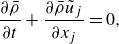
The fluctuation equations are far more complex than the incompressible counterparts. Following the derivation in Chen et al. (Reference Chen, Cheng, Gan and Fu2023b ), the fluctuation equations relative to (2.1) are written as
 $${\qquad \qquad \qquad \qquad \qquad \underbrace {\frac {\partial \rho ^{\prime }}{\partial t} + \frac {{\partial \bar {\rho } u_j^{{\prime \prime }}}}{\partial x_j} + \frac {\partial \rho ^{\prime } \tilde {u}_j }{\partial x_j}}_{\textit{linear terms}} = \underbrace {-\frac {\partial \rho ^{\prime } u_j^{{\prime \prime }}}{\partial x_j}}_{{\textit{nonlinear term}}},}$$
 $${\quad \begin{aligned}& \bar {\rho } \left ({ \frac {\partial u_i^{{\prime \prime }}}{\partial t} + \tilde {u}_j \frac {\partial u_i^{{\prime \prime }}}{\partial x_j} }\right ) + \big({ \rho ^{\prime } \tilde {u}_j + \bar {\rho } u_j^{{\prime \prime }}} \big) \frac {\partial \tilde {u}_i}{\partial x_j} + \frac {\partial p_{\textit {lin}}^{\prime }}{\partial x_i} - \frac {\partial \tau _{{i\!j},\textit {lin}}^{\prime }}{\partial x_j} \\[2pt] &\quad = \underbrace {- \frac {\partial }{\partial x_j} \left ({ \rho u_i^{{\prime \prime }} u_j^{{\prime \prime }} - \bar {\rho } \widetilde {u_i^{{\prime \prime }} u_j^{{\prime \prime }}} }\right )}_{{\textit{RSF}}} \underbrace {- \frac {\partial p_{\textit {nln}}^{\prime }}{\partial x_i}}_{\textit{PGNF}} + \underbrace {\frac {\partial \tau _{{i\!j},\textit {nln}}^{\prime }}{\partial x_j}}_{\textit{VSNF}} + \,\textit{MMNF}, \end{aligned}}$$
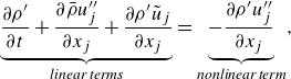
 \begin{aligned} & \bar {\rho } \left ({ c_v \frac {\partial T^{{\prime \prime }}}{\partial t} + c_p \tilde {u}_j \frac {\partial T^{{\prime \prime }}}{\partial x_j} }\right ) - R\widetilde {T} \frac {\partial \rho ^{\prime }}{\partial t} + \big({ \rho ^{\prime } \tilde {u}_j + \bar {\rho } u_j^{{\prime \prime }} }\big ) c_p \frac {\partial \widetilde {T}}{\partial x_j} - \left ( \tilde {u}_j \frac {\partial p_{\textit {lin}}^{\prime }}{\partial x_j} + u_j^{{\prime \prime }} \frac {\partial \bar {p}}{\partial x_j} \right ) \\[2pt] &\qquad + \frac {\partial \vartheta _{j,\textit {lin}}^{\prime }}{\partial x_j} - \bar {\tau }_{{i\!j},\textit {lin}} \frac {\partial u_i^{{\prime \prime }}}{\partial x_j} - \tau _{{i\!j},\textit {lin}}^{\prime } \frac {\partial \tilde {u}_i}{\partial x_j} = \underbrace {- c_p \frac {\partial }{\partial x_j} \left ({ \rho u_j^{{\prime \prime }} T^{{\prime \prime }} - \bar {\rho } \widetilde {u_j^{{\prime \prime }} T^{{\prime \prime }}} }\right )}_{\textit{THF}} \underbrace {- \frac {\partial \vartheta _{j,\textit {nln}}^{\prime }}{\partial x_j}}_{\textit{MHNF}} \\[2pt] &\qquad + \underbrace {\bar {\tau }_{{i\!j},\textit {nln}} \frac {\partial u_i^{{\prime \prime }}}{\partial x_j} + \tau _{{i\!j},\textit {nln}}^{\prime } \frac {\partial \tilde {u}_i}{\partial x_j} + \left ({ \tau _{{i\!j}}^{\prime } \frac {\partial u_i^{{\prime \prime }}}{\partial x_j} - \overline {\tau _{{i\!j}} \frac {\partial u_i^{{\prime \prime }}}{\partial x_j}} }\right )}_{\textit{VDNF}} + \,{\textit{PCNF}} + {\textit{EMNF}}. \end{aligned}
Here,
 $\varphi ^{\prime }$
and
$\varphi ^{\prime }$
and
 $\varphi ^{{\prime \prime }}$
are the Reynolds and Favre fluctuations, respectively; the linear and nonlinear fluctuation terms are listed on the two sides of each equation. There are five independent variables in the system. We choose the basic variable set as
$\varphi ^{{\prime \prime }}$
are the Reynolds and Favre fluctuations, respectively; the linear and nonlinear fluctuation terms are listed on the two sides of each equation. There are five independent variables in the system. We choose the basic variable set as
 ${\boldsymbol q}^{{\prime \prime }}=[\rho ^{\prime },\,u^{{\prime \prime }}, v^{{\prime \prime }},\,w^{{\prime \prime }},\,T^{{\prime \prime }}]^{T}$
, then the derived variables
${\boldsymbol q}^{{\prime \prime }}=[\rho ^{\prime },\,u^{{\prime \prime }}, v^{{\prime \prime }},\,w^{{\prime \prime }},\,T^{{\prime \prime }}]^{T}$
, then the derived variables
 $p^{\prime }$
,
$p^{\prime }$
,
 $\vartheta _j^{\prime }$
and
$\vartheta _j^{\prime }$
and
 $\tau _{{i\!j}}^{\prime }$
are not strictly linear functions of
$\tau _{{i\!j}}^{\prime }$
are not strictly linear functions of
 ${\boldsymbol q}^{{\prime \prime }}$
. To achieve a thorough linearisation of the system,
${\boldsymbol q}^{{\prime \prime }}$
. To achieve a thorough linearisation of the system,
 $p^{\prime }$
and
$p^{\prime }$
and
 $\vartheta _j^{\prime }$
are also divided into the linear and nonlinear parts in terms of
$\vartheta _j^{\prime }$
are also divided into the linear and nonlinear parts in terms of
 ${\boldsymbol q}^{{\prime \prime }}$
, as
${\boldsymbol q}^{{\prime \prime }}$
, as
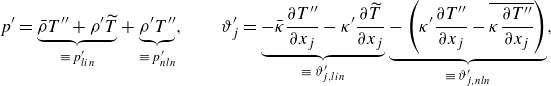 \begin{equation} p^{\prime } = \underbrace {\bar {\rho } T^{{\prime \prime }} + \rho ^{\prime } \widetilde {T}}_{\equiv\; p_{lin}^{\prime }} + \underbrace {\rho ^{\prime } T^{{\prime \prime }}}_{\equiv\; p_{nln}^{\prime }}, \qquad \vartheta _j^{\prime } = \underbrace {-\bar {\kappa } \frac {\partial T^{{\prime \prime }}}{\partial x_j} - \kappa ^{\prime } \frac {\partial \widetilde {T}}{\partial x_j}}_{\equiv\; \vartheta _{j,{lin}}^{\prime }} \underbrace {- \left ( \kappa ^{\prime } \frac {\partial T^{{\prime \prime }}}{\partial x_j} - \overline {\kappa \frac {\partial T^{{\prime \prime }}}{\partial x_j}} \right )}_{\equiv\; \vartheta _{j,{nln}}^{\prime }}, \end{equation}
and so is
 $\tau _{{i\!j}}^{\prime }=\tau _{{i\!j},\textit {lin}}^{\prime } + \tau _{{i\!j},\textit {nln}}^{\prime }$
(not detailed for brevity). As a result, the left-hand sides in (2.3) are all linear functions of
$\tau _{{i\!j}}^{\prime }=\tau _{{i\!j},\textit {lin}}^{\prime } + \tau _{{i\!j},\textit {nln}}^{\prime }$
(not detailed for brevity). As a result, the left-hand sides in (2.3) are all linear functions of
 ${\boldsymbol q}^{{\prime \prime }}$
, ready for constructing the linear operator. The various nonlinear fluctuation terms reside on the right-hand sides of (2.3), classified as underbraced. Their names are collectively defined in table 1. The expressions of the unspecified terms MMNF, PCNF, EMNF
are detailed in Appendix A.
${\boldsymbol q}^{{\prime \prime }}$
, ready for constructing the linear operator. The various nonlinear fluctuation terms reside on the right-hand sides of (2.3), classified as underbraced. Their names are collectively defined in table 1. The expressions of the unspecified terms MMNF, PCNF, EMNF
are detailed in Appendix A.
Table 1. Names and abbreviations of the nonlinear terms in the fluctuation equations.

Notably, the term RSF is the only nonlinear term in incompressible flows. For compressible cases, however, many other terms appear due to the thermodynamic processes. In previous works (e.g. Alizard et al. Reference Alizard, Pirozzoli, Bernardini and Grasso2015), RSF and THF were of the primary concern and were modelled using algebraic RANS relations to formulate the eLNS model; other terms were usually neglected. But here, we provide the complete form of the fluctuation equations and will clarify in § 4.1 the contribution of each nonlinear term.
2.2. The LNS and eLNS models
Equation (2.3) constitutes a closed set of equations for
 ${\boldsymbol q}^{{\prime \prime }}$
, and can be rearranged into an operator form as
${\boldsymbol q}^{{\prime \prime }}$
, and can be rearranged into an operator form as
 \begin{equation} \dfrac {\partial \rho ^{\prime }}{\partial t} - \mathcal{L}_\rho {\boldsymbol q}^{{\prime \prime }} = f_\rho ^{{\prime \prime }}, \quad \bar {\rho } \dfrac {\partial u_i^{{\prime \prime }}}{\partial t} - \mathcal{L}_{m_i} {\boldsymbol q}^{{\prime \prime }} = f_{m_i}^{{\prime \prime }}, \quad \bar {\rho } c_v \dfrac {\partial T^{{\prime \prime }}}{\partial t} - R\widetilde {T} \dfrac {\partial \rho ^{\prime }}{\partial t} - \mathcal{L}_{h} {\boldsymbol q}^{{\prime \prime }} = f_h^{{\prime \prime }}, \end{equation}
where
 $\mathcal{L}$
denotes the linear operator determined only by the mean flow
$\mathcal{L}$
denotes the linear operator determined only by the mean flow
 $\widetilde {\boldsymbol q}$
, and
$\widetilde {\boldsymbol q}$
, and
 $f^{{\prime \prime }}$
represents the nonlinear terms. Detailed expressions of
$f^{{\prime \prime }}$
represents the nonlinear terms. Detailed expressions of
 $\mathcal{L}$
are readily contained in (2.3), also available in Dawson & McKeon (Reference Dawson and McKeon2020) and Chen et al. (Reference Chen, Cheng, Fu and Gan2023a
). Equation (2.5a
) is rewritten into a matrix form as
$\mathcal{L}$
are readily contained in (2.3), also available in Dawson & McKeon (Reference Dawson and McKeon2020) and Chen et al. (Reference Chen, Cheng, Fu and Gan2023a
). Equation (2.5a
) is rewritten into a matrix form as
 \begin{equation} \boldsymbol{A} \frac {\partial }{\partial t} \left [\!\begin{array}{*{20}{c}} \rho ^{\prime } \\ u_j^{{\prime \prime }} \\ T^{{\prime \prime }} \end{array}\!\right ] = \left [\!\begin{array}{*{20}{c}} \mathcal{L}_\rho \\ \mathcal{L}_{m_i} \\ \mathcal{L}_{h} \end{array}\!\right ] {\boldsymbol q}^{{\prime \prime }} + \left [\!\begin{array}{*{20}{c}} f_\rho ^{{\prime \prime }} \\ f_{m_i}^{{\prime \prime }} \\ f_h^{{\prime \prime }} \end{array}\!\right ], \qquad \boldsymbol{A} \equiv \left [ \begin{array}{*{20}{c}} 1&{}&{}\\ {}&\bar {\rho }\delta _{{i\!j}}&{} \\ -R\widetilde {T}&{}&\bar {\rho } c_v \end{array} \right ], \end{equation}
or equivalently
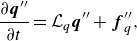 \begin{equation} \frac {\partial {\boldsymbol q}^{{\prime \prime }}}{\partial t} = \mathcal{L}_q {\boldsymbol q}^{{\prime \prime }} + {\boldsymbol f}_q^{{\prime \prime }}, \end{equation}
where
 $\boldsymbol{A}^{-1}$
has been absorbed into
$\boldsymbol{A}^{-1}$
has been absorbed into
 $\mathcal{L}_q$
and
$\mathcal{L}_q$
and
 ${\boldsymbol f}_q^{{\prime \prime }}\equiv [f_\rho ^{{\prime \prime }},\,f_u^{{\prime \prime }},\,f_v^{{\prime \prime }},\,f_w^{{\prime \prime }},\,f_T^{{\prime \prime }}]^{\textrm{T}}$
. Equation (2.6) is the linearised NS equation and serves as a classic model problem. The linear model built upon (2.6) is often referred to as the LNS model.
${\boldsymbol f}_q^{{\prime \prime }}\equiv [f_\rho ^{{\prime \prime }},\,f_u^{{\prime \prime }},\,f_v^{{\prime \prime }},\,f_w^{{\prime \prime }},\,f_T^{{\prime \prime }}]^{\textrm{T}}$
. Equation (2.6) is the linearised NS equation and serves as a classic model problem. The linear model built upon (2.6) is often referred to as the LNS model.
In addition to the LNS model, the compressible eLNS model is frequently considered for model improvement, which is built upon algebraic RANS models (Alizard et al. Reference Alizard, Pirozzoli, Bernardini and Grasso2015; Chen et al. Reference Chen, Gan and Fu2024, Reference Chen, Gan and Fu2025). Specifically, the Boussinesq assumption and the strong Reynolds analogy (SRA) are introduced to linearise the Reynolds stress
 $\tau _{R,{i\!j}}$
and turbulent heat flux
$\tau _{R,{i\!j}}$
and turbulent heat flux
 $\vartheta _{R,j}$
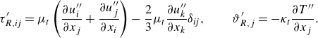 \begin{equation} \tau _{R,{i\!j}}^{\prime } = \mu _t \left ({ \frac {\partial u_i^{{\prime \prime }}}{\partial x_j} + \frac {\partial u_j^{{\prime \prime }}}{\partial x_i} }\right ) - \frac {2}{3}\mu _t \frac {\partial u_k^{{\prime \prime }}}{\partial x_k} \delta _{{i\!j}}, \qquad \vartheta _{R,j}^{\prime } = -\kappa _t \frac {\partial T^{{\prime \prime }}}{\partial x_j}. \end{equation}
Here,
 $\kappa _t$
is the eddy diffusivity. In practice,
$\kappa _t$
is the eddy diffusivity. In practice,
 $\mu _t$
and
$\mu _t$
and
 $\kappa _t$
are either assumed known from the DNS data or from semi-empirical models (e.g. Fan et al. Reference Fan, Kozul, Li and Sandberg2024). The terms
$\kappa _t$
are either assumed known from the DNS data or from semi-empirical models (e.g. Fan et al. Reference Fan, Kozul, Li and Sandberg2024). The terms
 $\tau _R^{\prime }$
and
$\tau _R^{\prime }$
and
 $\vartheta _R^{\prime }$
were originally designed to partially model the colour of the nonlinear terms. Taking the RSF term as an example, it is modelled as
$\vartheta _R^{\prime }$
were originally designed to partially model the colour of the nonlinear terms. Taking the RSF term as an example, it is modelled as
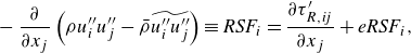 \begin{equation} -\frac {\partial }{\partial x_j} \left ({ \rho u_i^{{\prime \prime }} u_j^{{\prime \prime }} - \bar {\rho } \widetilde {u_i^{{\prime \prime }} u_j^{{\prime \prime }}} }\right ) \equiv {\textit{RSF}}_i = \frac {\partial \tau _{R,{i\!j}}^{\prime }}{\partial x_j} + {\textit{eRSF}}_i, \end{equation}
where
 ${\rm eRSF}$
represents the residual nonlinear term of RSF, after subtracting the modelled stress flux
${\rm eRSF}$
represents the residual nonlinear term of RSF, after subtracting the modelled stress flux
 ${\partial \tau _{R,{i\!j}}^{\prime }}/{\partial x_j}$
. The other two residual terms
${\partial \tau _{R,{i\!j}}^{\prime }}/{\partial x_j}$
. The other two residual terms
 $\rm{eTHF}$
and
$\rm{eTHF}$
and
 ${\rm eVDNF}$
, after modelling the turbulent heat flux and viscous dissipation, are similarly defined (e.g. Chen et al. Reference Chen, Cheng, Gan and Fu2023b
).
${\rm eVDNF}$
, after modelling the turbulent heat flux and viscous dissipation, are similarly defined (e.g. Chen et al. Reference Chen, Cheng, Gan and Fu2023b
).
It is worth emphasising that (2.8) is the core assumption for the eLNS model. However, we will show in § 4 that (2.8) can deviate from its original intention. The supposedly small residual terms,
 ${\rm{eRSF}}$
and
${\rm{eRSF}}$
and
 $\rm{eTHF}$
, turn out to essentially rebuild the forcing distributions.
$\rm{eTHF}$
, turn out to essentially rebuild the forcing distributions.
Since
 $\mu _t$
and
$\mu _t$
and
 $\kappa _t$
profiles are assumed fixed,
$\kappa _t$
profiles are assumed fixed,
 $\tau _R^{\prime }$
and
$\tau _R^{\prime }$
and
 $\vartheta _R^{\prime }$
are linear in terms of
$\vartheta _R^{\prime }$
are linear in terms of
 ${\boldsymbol q}^{{\prime \prime }}$
, so these eddy-viscosity-related terms in the momentum and enthalpy equations are linearised as
${\boldsymbol q}^{{\prime \prime }}$
, so these eddy-viscosity-related terms in the momentum and enthalpy equations are linearised as
 \begin{equation} \frac {\partial \tau _{R,{i\!j}}^{\prime }}{\partial x_j} \equiv \mathcal{M}_{m_i} {\boldsymbol q}^{{\prime \prime }}, \quad - \frac {\partial \vartheta _{R,j}^{\prime }}{\partial x_j} + \bar {\tau }_{R,{i\!j}} \frac {\partial u_i^{{\prime \prime }}}{\partial x_j} + \tau _{R,{i\!j}}^{\prime } \frac {\partial \tilde {u}_i}{\partial x_j} \equiv \mathcal{M}_{h} {\boldsymbol q}^{{\prime \prime }}. \end{equation}
Consequently, parts of the LNS nonlinear terms can be linearised and moved into the linear operator, so that the model is eddy-viscosity enhanced, following the term for incompressible flows (Madhusudanan, Illingworth & Marusic Reference Madhusudanan, Illingworth and Marusic2019). The resulting operator form of the eLNS model reads
 \begin{equation} \left \{ \!\!\begin{array}{l} \dfrac {\partial \rho ^{\prime }}{\partial t} = \mathcal{E}_\rho {\boldsymbol q}^{{\prime \prime }} + e_\rho ^{{\prime \prime }}, \quad \text{with $\mathcal{E}_{\rho }\equiv \mathcal{L}_{\rho }$ and $e_\rho ^{{\prime \prime }}\equiv f_\rho ^{{\prime \prime }}$},\\[10pt] \displaystyle \bar {\rho } \dfrac {\partial u_i^{{\prime \prime }}}{\partial t} = \underbrace {\left ( \mathcal{L}_{m_i} + \mathcal{M}_{m_i} \right )}_{\equiv\; \mathcal{E}_{m_i}} {\boldsymbol q}^{{\prime \prime }} + \underbrace {\left ( f_{m_i}^{{\prime \prime }} - \mathcal{M}_{m_i} {\boldsymbol q}^{{\prime \prime }} \right )}_{\equiv\; e_{m_i}^{{\prime \prime }}},\\[10pt] \displaystyle \bar {\rho } c_v \dfrac {\partial T^{{\prime \prime }}}{\partial t} - R\widetilde {T} \dfrac {\partial \rho ^{\prime }}{\partial t} = \underbrace {\left ( \mathcal{L}_{h} + \mathcal{M}_{h} \right )}_{\equiv\; \mathcal{E}_{h}} {\boldsymbol q}^{{\prime \prime }} + \underbrace {\left ( f_{h}^{{\prime \prime }} - \mathcal{M}_{h} {\boldsymbol q}^{{\prime \prime }} \right )}_{\equiv\; e_{h}^{{\prime \prime }}}, \end{array} \right . \end{equation}
where the linear operator
 $\mathcal{E}$
and the nonlinear term
$\mathcal{E}$
and the nonlinear term
 ${\boldsymbol e}^{{\prime \prime }}$
for eLNS are defined as underbraced. The final standard form similar to (2.6) is
${\boldsymbol e}^{{\prime \prime }}$
for eLNS are defined as underbraced. The final standard form similar to (2.6) is
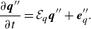 \begin{equation} \frac {\partial {\boldsymbol q}^{{\prime \prime }}}{\partial t} = \mathcal{E}_q {\boldsymbol q}^{{\prime \prime }} + {\boldsymbol e}_q^{{\prime \prime }}. \end{equation}
Note that
 $\mathcal{E}_q$
is the same as
$\mathcal{E}_q$
is the same as
 $\mathcal{L}_q$
except for replacing
$\mathcal{L}_q$
except for replacing
 $\,\bar {\!\mu }$
with
$\,\bar {\!\mu }$
with
 $\,\bar {\!\mu }+\mu _t$
and
$\,\bar {\!\mu }+\mu _t$
and
 $\bar {\kappa }$
with
$\bar {\kappa }$
with
 $\bar {\kappa }+\kappa _t$
. Equations (2.6) and (2.11) constitute the model equations for LNS and eLNS, respectively.
$\bar {\kappa }+\kappa _t$
. Equations (2.6) and (2.11) constitute the model equations for LNS and eLNS, respectively.
It is worth mentioning that the eLNS model was originally derived based on the triple decomposition of
 $\boldsymbol q$
(Reynolds & Hussain Reference Reynolds and Hussain1972; Alizard et al. Reference Alizard, Pirozzoli, Bernardini and Grasso2015), where
$\boldsymbol q$
(Reynolds & Hussain Reference Reynolds and Hussain1972; Alizard et al. Reference Alizard, Pirozzoli, Bernardini and Grasso2015), where
 $\boldsymbol q$
is decomposed into the mean part, the turbulent fluctuation part and a small-amplitude organised perturbation. This approach is more physically interpretable, whereas the final linearised equation is mathematically equivalent to (2.11). Therefore, we do not present the triply
decomposed fluctuation equations, considering the already complicated (2.3).
$\boldsymbol q$
is decomposed into the mean part, the turbulent fluctuation part and a small-amplitude organised perturbation. This approach is more physically interpretable, whereas the final linearised equation is mathematically equivalent to (2.11). Therefore, we do not present the triply
decomposed fluctuation equations, considering the already complicated (2.3).
2.3. The DNS datasets
A series of DNSs for compressible turbulent channel flows have been conducted by the present authors’ group, as described at length in Cheng & Fu (Reference Cheng and Fu2022, Reference Cheng and Fu2023). The simulations adopt three bulk Mach numbers
 ${\textit {Ma}}_b=U_b/a_w=0.8, 1.5, 3.0$
and a series of bulk Reynolds numbers
${\textit {Ma}}_b=U_b/a_w=0.8, 1.5, 3.0$
and a series of bulk Reynolds numbers
 $\textit{Re}_b=\rho _b U_b h/\mu _w$
. Here,
$\textit{Re}_b=\rho _b U_b h/\mu _w$
. Here,
 $\rho _b$
and
$\rho _b$
and
 $U_b$
are the bulk density and streamwise velocity,
$U_b$
are the bulk density and streamwise velocity,
 $a=(\gamma R T)^{1/2}$
is the speed of sound with the specific ratio
$a=(\gamma R T)^{1/2}$
is the speed of sound with the specific ratio
 $\gamma =1.4$
,
$\gamma =1.4$
,
 $h$
is the channel half-width and the subscript
$h$
is the channel half-width and the subscript
 $w$
denotes wall quantities. Our focus is the compressibility effects on the forcing models, so we first select two DNS cases at
$w$
denotes wall quantities. Our focus is the compressibility effects on the forcing models, so we first select two DNS cases at
 ${\textit {Ma}}_b=1.5$
and 3.0 with nearly equal
${\textit {Ma}}_b=1.5$
and 3.0 with nearly equal
 $\textit{Re}_\tau ^*$
. A third case with a higher
$\textit{Re}_\tau ^*$
. A third case with a higher
 $\textit{Re}$
at
$\textit{Re}$
at
 ${\textit {Ma}}_b=1.5$
is also included, to examine potential scalings. Additionally, two incompressible DNS cases at different
${\textit {Ma}}_b=1.5$
is also included, to examine potential scalings. Additionally, two incompressible DNS cases at different
 $\textit{Re}_\tau$
are adopted, with data from Ying et al. (Reference Ying, Liang, Li and Fu2023), to facilitate quantitative measure of the compressibility effects. Detailed parameters of the five cases are listed in table 2. Here,
$\textit{Re}_\tau$
are adopted, with data from Ying et al. (Reference Ying, Liang, Li and Fu2023), to facilitate quantitative measure of the compressibility effects. Detailed parameters of the five cases are listed in table 2. Here,
 $\textit{Re}_\tau =\rho _w u_\tau h/\mu _w$
and
$\textit{Re}_\tau =\rho _w u_\tau h/\mu _w$
and
 $\textit{Re}_\tau ^*=\bar {\rho }u_\tau ^* h/\,\bar {\!\mu }$
are the friction and semi-local Reynolds numbers;
$\textit{Re}_\tau ^*=\bar {\rho }u_\tau ^* h/\,\bar {\!\mu }$
are the friction and semi-local Reynolds numbers;
 $u_\tau$
is the friction velocity and
$u_\tau$
is the friction velocity and
 $u_\tau ^*$
is the semi-local counterpart;
$u_\tau ^*$
is the semi-local counterpart;
 $\widetilde {T}_c$
is the temperature at the channel centre;
$\widetilde {T}_c$
is the temperature at the channel centre;
 $L_x$
and
$L_x$
and
 $L_z$
are the domain sizes. For later use, the wall viscous and semi-local length scales are defined as
$L_z$
are the domain sizes. For later use, the wall viscous and semi-local length scales are defined as
 $\delta _\nu =\mu _w/(\rho _wu_\tau )$
and
$\delta _\nu =\mu _w/(\rho _wu_\tau )$
and
 $\delta _\nu ^*=\,\bar {\!\mu }/(\bar {\rho }u_\tau ^*)$
, based on which the two sets of non-dimensional lengths are denoted by superscripts
$\delta _\nu ^*=\,\bar {\!\mu }/(\bar {\rho }u_\tau ^*)$
, based on which the two sets of non-dimensional lengths are denoted by superscripts
 $+$
and
$+$
and
 $*$
, respectively.
$*$
, respectively.
Table 2. Parameters of the DNS cases for turbulent channel flows, where
 $t_{\textit {total}} u_{\tau }/h$
is the total eddy turnover time to accumulate statistics. Two incompressible cases are also included for later reference.
$t_{\textit {total}} u_{\tau }/h$
is the total eddy turnover time to accumulate statistics. Two incompressible cases are also included for later reference.

To obtain the real forcing statistics, the nonlinear terms
 ${\boldsymbol f}_q^{{\prime \prime }}$
and
${\boldsymbol f}_q^{{\prime \prime }}$
and
 ${\boldsymbol e}_q^{{\prime \prime }}$
are calculated by their definitions in §§ 2.1, 2.2 using the DNS data. The linear models in this work are solved within the framework of the stochastic Lyapunov equation (see § 2.4), so we do not need time-resolved DNS data of massive memory requirement as in Morra et al. (Reference Morra, Nogueira, Cavalieri and Henningson2021) and Ying et al. (Reference Ying, Chen, Li and Fu2024a
) for incompressible cases. Instead, we focus on the ensemble (temporal) average
${\boldsymbol e}_q^{{\prime \prime }}$
are calculated by their definitions in §§ 2.1, 2.2 using the DNS data. The linear models in this work are solved within the framework of the stochastic Lyapunov equation (see § 2.4), so we do not need time-resolved DNS data of massive memory requirement as in Morra et al. (Reference Morra, Nogueira, Cavalieri and Henningson2021) and Ying et al. (Reference Ying, Chen, Li and Fu2024a
) for incompressible cases. Instead, we focus on the ensemble (temporal) average
 $\langle \cdot \rangle$
of variables, where time-not-resolved data are adequate. Therefore, the sampling number of the instantaneous fields
$\langle \cdot \rangle$
of variables, where time-not-resolved data are adequate. Therefore, the sampling number of the instantaneous fields
 $N_t$
can be orders of magnitude lower than that required by the time-resolved data; for the latter case,
$N_t$
can be orders of magnitude lower than that required by the time-resolved data; for the latter case,
 $N_t$
can reach
$N_t$
can reach
 ${\sim}10^4$
at current
${\sim}10^4$
at current
 $\textit{Re}_\tau$
. The price is that the frequency spectrum is not resolved, but we can still reveal the forcing statistics in the spatial spectra, which provides adequate information to improve the stochastic linear models. The Fourier decomposition is applied on
$\textit{Re}_\tau$
. The price is that the frequency spectrum is not resolved, but we can still reveal the forcing statistics in the spatial spectra, which provides adequate information to improve the stochastic linear models. The Fourier decomposition is applied on
 ${\boldsymbol q}^{{\prime \prime }}$
in two homogenous directions as
${\boldsymbol q}^{{\prime \prime }}$
in two homogenous directions as
 \begin{equation} {\boldsymbol q}^{{\prime \prime }}\! \left (x,y,z,t\right ) = \iint \nolimits _{-\infty }^{\infty } {\hat {\boldsymbol q}^{{\kern0.3pt}{\prime \prime }} \left (y, t; k_x, k_z\right ) \exp \left [{\mathrm{i}} \left (k_x x + k_z z\right )\right ] {\mathrm{d}} k_x {\mathrm{d}} k_z}, \end{equation}
where
 $k_x$
and
$k_x$
and
 $k_z$
are the streamwise and spanwise wavenumbers, and
$k_z$
are the streamwise and spanwise wavenumbers, and
 $\hat {\boldsymbol q}^{{\kern0.3pt}{\prime \prime }}$
is the shape function. The Fourier components of
$\hat {\boldsymbol q}^{{\kern0.3pt}{\prime \prime }}$
is the shape function. The Fourier components of
 $\,\hat {\!\boldsymbol f}^{{\prime \prime }}$
and
$\,\hat {\!\boldsymbol f}^{{\prime \prime }}$
and
 $\,\hat {\!\boldsymbol e}^{{\prime \prime }}$
are similarly defined. Thevalue of
$\,\hat {\!\boldsymbol e}^{{\prime \prime }}$
are similarly defined. Thevalue of
 $N_t$
used for different cases is listed in table 2, which will be shown in § 3 to be large enough to provide converged spectral statistics.
$N_t$
used for different cases is listed in table 2, which will be shown in § 3 to be large enough to provide converged spectral statistics.
2.4. Fluctuations in response to modelled and DNS forcing
In this subsection, we first present how the spectral correlation tensor
 $\widehat {\boldsymbol{\Phi }}(y,y^{\prime };k_x,k_z)= \langle \hat {\boldsymbol q}^{{\kern0.3pt}{\prime \prime }}(y,t;k_x,k_z) \hat {\boldsymbol q}^{{{\prime \prime }}{{H}}}(y^{\prime },t;k_x,k_z) \rangle$
in response to a modelled forcing is obtained in the linear model, which requires only the mean flow (including
$\widehat {\boldsymbol{\Phi }}(y,y^{\prime };k_x,k_z)= \langle \hat {\boldsymbol q}^{{\kern0.3pt}{\prime \prime }}(y,t;k_x,k_z) \hat {\boldsymbol q}^{{{\prime \prime }}{{H}}}(y^{\prime },t;k_x,k_z) \rangle$
in response to a modelled forcing is obtained in the linear model, which requires only the mean flow (including
 $\mu _t$
,
$\mu _t$
,
 $\kappa _t$
) as the input. Afterwards, we present how the real forcing can be computed from the DNS data, hence enabling a direct interpretation of the model errors.
$\kappa _t$
) as the input. Afterwards, we present how the real forcing can be computed from the DNS data, hence enabling a direct interpretation of the model errors.
In the Fourier space, the model equations (2.6) and (2.11) are expressed as
 \begin{equation} \frac {\partial \hat {\boldsymbol q}^{{\kern0.3pt}{\prime \prime }}}{\partial t} = \widehat {\mathcal{L}}_q \hat {\boldsymbol q}^{{\kern0.3pt}{\prime \prime }} + \,\hat {\!\boldsymbol f}_q^{{\prime \prime }}, \qquad \frac {\partial \hat {\boldsymbol q}^{{\kern0.3pt}{\prime \prime }}}{\partial t} = \widehat {\mathcal{E}}_q \hat {\boldsymbol q}^{{\kern0.3pt}{\prime \prime }} + \,\hat {\!\boldsymbol e}_q^{{\prime \prime }}. \end{equation}
When the real forcings
 $\,\hat {\!\boldsymbol f}_q^{{\prime \prime }}$
and
$\,\hat {\!\boldsymbol f}_q^{{\prime \prime }}$
and
 $\,\hat {\!\boldsymbol e}_q^{{\prime \prime }}$
are unknown, the stochastic linear models provide a mean to estimate
$\,\hat {\!\boldsymbol e}_q^{{\prime \prime }}$
are unknown, the stochastic linear models provide a mean to estimate
 $\widehat {\boldsymbol{\Phi }}$
. An idealised stochastic forcing is assumed as
$\widehat {\boldsymbol{\Phi }}$
. An idealised stochastic forcing is assumed as
 $\,\hat {\!\boldsymbol f}_q=\boldsymbol{F}\,\hat {\!\boldsymbol f}_0$
(so is
$\,\hat {\!\boldsymbol f}_q=\boldsymbol{F}\,\hat {\!\boldsymbol f}_0$
(so is
 $\,\hat {\!\boldsymbol e}_q=\boldsymbol{E}\,\hat {\!\boldsymbol e}_0$
), where the matrix
$\,\hat {\!\boldsymbol e}_q=\boldsymbol{E}\,\hat {\!\boldsymbol e}_0$
), where the matrix
 $\boldsymbol{F}(y)$
models the wall-normally varied forcing amplitude, and
$\boldsymbol{F}(y)$
models the wall-normally varied forcing amplitude, and
 $\,\hat {\!\boldsymbol f}_0$
(and
$\,\hat {\!\boldsymbol f}_0$
(and
 $\,\hat {\!\boldsymbol e}_0$
) is a delta-correlated Gaussian white noise with zero mean. Consequently, the correlation tensor
$\,\hat {\!\boldsymbol e}_0$
) is a delta-correlated Gaussian white noise with zero mean. Consequently, the correlation tensor
 $\widehat {\boldsymbol{\Phi }}$
is obtained by solving the Lyapunov equation (Farrell & Ioannou Reference Farrell and Ioannou1993), as
$\widehat {\boldsymbol{\Phi }}$
is obtained by solving the Lyapunov equation (Farrell & Ioannou Reference Farrell and Ioannou1993), as
 $${\widehat {\mathcal{L}}\, \widehat {\boldsymbol{\Phi }} + \widehat {\boldsymbol{\Phi }} \widehat {\mathcal{L}}^{{H}} + (\boldsymbol{{FF}}^{{H}}) = \boldsymbol{0}, \qquad \text{for the LNS model},}$$
 $${\widehat {\mathcal{E}}\, \widehat {\boldsymbol{\Phi }} + \widehat {\boldsymbol{\Phi }} \widehat {\mathcal{E}}^{{H}} + (\boldsymbol{{EE}}^{{H}}) = \boldsymbol{0}, \qquad \text{for the eLNS model},}$$
where the Hermitian transpose of
 $\widehat {\mathcal{L}}$
and
$\widehat {\mathcal{L}}$
and
 $\widehat {\mathcal{E}}$
is defined as the discrete adjoint. In the simplest models,
$\widehat {\mathcal{E}}$
is defined as the discrete adjoint. In the simplest models,
 $\boldsymbol{F}$
and
$\boldsymbol{F}$
and
 $\boldsymbol{E}$
are assumed to be diagonal, suggesting perfect zero
correlation of the forcing between different variables and between different wall-normal heights. The simple yet well-behaved W-model (Gupta et al. Reference Gupta, Madhusudanan, Wan, Illingworth and Juniper2021; Chen et al. Reference Chen, Cheng, Gan and Fu2023b
) is considered here, where the forcing amplitude varies in proportion to the kinematic eddy viscosity
$\boldsymbol{E}$
are assumed to be diagonal, suggesting perfect zero
correlation of the forcing between different variables and between different wall-normal heights. The simple yet well-behaved W-model (Gupta et al. Reference Gupta, Madhusudanan, Wan, Illingworth and Juniper2021; Chen et al. Reference Chen, Cheng, Gan and Fu2023b
) is considered here, where the forcing amplitude varies in proportion to the kinematic eddy viscosity
 $\nu _t=\mu _t/\bar {\rho }$
, as
$\nu _t=\mu _t/\bar {\rho }$
, as
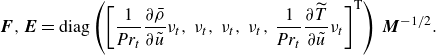 \begin{equation} \boldsymbol{F},\boldsymbol{E} = \text{diag} \left ( \left [\frac {1}{{\textit {Pr}}_t} \frac {\partial \bar {\rho }}{\partial \tilde {u}} \nu _t,\; \nu _t,\; \nu _t,\; \nu _t,\; \frac {1}{{\textit {Pr}}_t} \frac {\partial \widetilde {T}}{\partial \tilde {u}} \nu _t\right ]^{\textrm{T}} \right ) \,\boldsymbol{M}^{-1/2}. \end{equation}
The weight matrix
 $\boldsymbol{M}$
will be defined later, and the extended SRA (Huang, Coleman & Bradshaw Reference Huang, Coleman and Bradshaw1995) has been utilised in deriving (2.15) as
$\boldsymbol{M}$
will be defined later, and the extended SRA (Huang, Coleman & Bradshaw Reference Huang, Coleman and Bradshaw1995) has been utilised in deriving (2.15) as
 \begin{equation} T^{{\prime \prime }}_{\textit {rms}} \approx \frac {1}{{\textit {Pr}}_t} \left |\frac {\partial \widetilde {T}}{\partial \tilde {u}} \right | u^{{\prime \prime }}_{\textit {rms}}, \qquad \rho ^{\prime }_{\textit {rms}} \approx \frac {1}{{\textit {Pr}}_t} \left |\frac {\partial \bar {\rho }}{\partial \tilde {u}}\right | u^{{\prime \prime }}_{\textit {rms}}, \end{equation}
where
 $rms$
denotes the root mean square. Equation (2.16) also suggests two wall viscous units for the temperature and density,
$rms$
denotes the root mean square. Equation (2.16) also suggests two wall viscous units for the temperature and density,
 $T_\tau =(\partial \widetilde {T}/\partial \tilde {u})_w u_\tau /{\textit {Pr}}$
and
$T_\tau =(\partial \widetilde {T}/\partial \tilde {u})_w u_\tau /{\textit {Pr}}$
and
 $\rho _\tau =(\partial \bar {\rho }/\partial \tilde {u})_w u_\tau$
.
$\rho _\tau =(\partial \bar {\rho }/\partial \tilde {u})_w u_\tau$
.
The eigenmodes of
 $\widehat {\boldsymbol{\Phi }}$
, known as the proper orthogonal decomposition (POD) or Karhunen–Loève modes, are of interest in various analyses on turbulence. They are defined as
$\widehat {\boldsymbol{\Phi }}$
, known as the proper orthogonal decomposition (POD) or Karhunen–Loève modes, are of interest in various analyses on turbulence. They are defined as
 \begin{equation} \left(\widehat {\boldsymbol{\Phi }}, \,\check {\!\boldsymbol q}_j^{{\prime \prime }}\right)_E = \theta _j \,\check {\!\boldsymbol q}_j^{{\prime \prime }}, \qquad j =1,2,\ldots , \end{equation}
where the eigenvalues and eigenfunctions
 $\theta _j$
and
$\theta _j$
and
 $\,\check {\!\boldsymbol q}_j^{{\prime \prime }}$
are sorted in the descending order of the energy of the
$\,\check {\!\boldsymbol q}_j^{{\prime \prime }}$
are sorted in the descending order of the energy of the
 $j$
th mode (
$j$
th mode (
 $\theta _j$
). These POD modes are orthogonal to each other under the energy norm
$\theta _j$
). These POD modes are orthogonal to each other under the energy norm
 $(\cdot ,\cdot )_E$
, which is defined following common usage (Chu Reference Chu1965) as
$(\cdot ,\cdot )_E$
, which is defined following common usage (Chu Reference Chu1965) as
 \begin{equation} \|\,\check {\!\boldsymbol q}^{{\prime \prime }}\|^2 = \left( \,\check {\!\boldsymbol q}^{{\prime \prime }}, \,\check {\!\boldsymbol q}^{{\prime \prime }} \right)_E = \int _{0}^{2h} { \left ( \bar {\rho } \,\check {\!\boldsymbol u}^{{{\prime \prime }}{{H}}} \,\check {\!\boldsymbol u}^{{\prime \prime }} + \frac {R \widetilde {T}}{\bar {\rho }} \check {\rho }^{{\prime }\dagger } \check {\rho }^{\prime } + \frac {\bar {\rho } c_v}{\widetilde {T}} \check {T}^{{{\prime \prime }}\dagger } \widehat {T}^{{\prime \prime }} \right ) {\mathrm{d}} y} = \,\check {\!\boldsymbol Q}^{{{\prime \prime }}{{H}}} \boldsymbol{M} \,\check {\!\boldsymbol Q}^{{\prime \prime }}. \end{equation}
Here,
 $\dagger$
denotes complex conjugate, the global vector
$\dagger$
denotes complex conjugate, the global vector
 $\,\check {\!\boldsymbol Q}^{{\prime \prime }}$
contains
$\,\check {\!\boldsymbol Q}^{{\prime \prime }}$
contains
 $\,\check {\!\boldsymbol q}^{{\prime \prime }}$
at all wall-normal grids and
$\,\check {\!\boldsymbol q}^{{\prime \prime }}$
at all wall-normal grids and
 $\boldsymbol{M}$
is the weight matrix. Regarding the numerics, (2.14) is discretised using the Chebyshev collocation point method; 241 points are used in default, which is abundant to ensure grid independence. The solver verification can be found in Chen et al. (Reference Chen, Cheng, Fu and Gan2023a
).
$\boldsymbol{M}$
is the weight matrix. Regarding the numerics, (2.14) is discretised using the Chebyshev collocation point method; 241 points are used in default, which is abundant to ensure grid independence. The solver verification can be found in Chen et al. (Reference Chen, Cheng, Fu and Gan2023a
).
Instead of the ideal modelling in (2.15), the forcings can be realistically computed by their definitions from the DNS data. Equation (2.13) indicates that the correlation tensor satisfies the following two Lyapunov equations for the LNS and eLNS models, respectively (derivations in Appendix A):
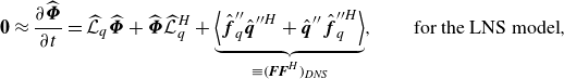 $${{\boldsymbol 0} \approx \dfrac {\partial \widehat {\boldsymbol{\Phi }}}{\partial t} = \widehat {\mathcal{L}}_q \widehat {\boldsymbol{\Phi }} + \widehat {\boldsymbol{\Phi }} \widehat {\mathcal{L}}_q^{{H}} + \underbrace {\left\langle \,\hat {\!\boldsymbol f}_q^{{\prime \prime }} \hat {\boldsymbol q}^{{{\prime \prime }}{{H}}} + \hat {\boldsymbol q}^{{\kern0.3pt}{\prime \prime }} \,\hat {\!\boldsymbol f}_q^{{{\prime \prime }}{{H}}} \right\rangle }_{\equiv (\boldsymbol{{FF}}^{{H}})_{\textit{DNS}}},\qquad \text{for the LNS model},}$$
 $${{\boldsymbol 0} \approx \dfrac {\partial \widehat {\boldsymbol{\Phi }}}{\partial t} = \widehat {\mathcal{E}}_q \widehat {\boldsymbol{\Phi }} + \widehat {\boldsymbol{\Phi }} \widehat {\mathcal{E}}_q^{{H}} + \underbrace {\left\langle \,\hat {\!\boldsymbol e}_q^{{\prime \prime }} \hat {\boldsymbol q}^{{{\prime \prime }}{{H}}} + \hat {\boldsymbol q}^{{\kern0.3pt}{\prime \prime }} \,\hat {\!\boldsymbol e}_q^{{{\prime \prime }}{{H}}} \right\rangle }_{\equiv (\boldsymbol{{EE}}^{{H}})_{\textit{DNS}}},\qquad \text{for the eLNS model}.}$$
Here, the approximation on the left-hand side holds subject to a sufficiently large
 $N_t$
. Comparing between (2.14), (2.19), we can define the real forcing matrix from DNS as
$N_t$
. Comparing between (2.14), (2.19), we can define the real forcing matrix from DNS as
 $(\boldsymbol{{FF}}^{{H}})_{\textit{DNS}}$
and
$(\boldsymbol{{FF}}^{{H}})_{\textit{DNS}}$
and
 $(\boldsymbol{{EE}}^{{H}})_{\textit{DNS}}$
, as underbraced in (2.19). A reasonable consequence is that when
$(\boldsymbol{{EE}}^{{H}})_{\textit{DNS}}$
, as underbraced in (2.19). A reasonable consequence is that when
 $(\boldsymbol{{FF}}^{{H}})_{\textit{DNS}}$
and
$(\boldsymbol{{FF}}^{{H}})_{\textit{DNS}}$
and
 $(\boldsymbol{{EE}}^{{H}})_{\textit{DNS}}$
are input into the stochastic linear models (2.14), the output
$(\boldsymbol{{EE}}^{{H}})_{\textit{DNS}}$
are input into the stochastic linear models (2.14), the output
 $\widehat {\boldsymbol{\Phi }}$
should be identical to the DNS counterpart
$\widehat {\boldsymbol{\Phi }}$
should be identical to the DNS counterpart
 $\widehat {\boldsymbol{\Phi }}_{\textit{DNS}}$
, which is required by the models’ mathematical self-consistency. On the other hand,
$\widehat {\boldsymbol{\Phi }}_{\textit{DNS}}$
, which is required by the models’ mathematical self-consistency. On the other hand,
 $(\boldsymbol{{FF}}^{{H}})_{\textit{DNS}}$
and
$(\boldsymbol{{FF}}^{{H}})_{\textit{DNS}}$
and
 $(\boldsymbol{{EE}}^{{H}})_{\textit{DNS}}$
naturally provide the ‘standard answers’ to how to model
$(\boldsymbol{{EE}}^{{H}})_{\textit{DNS}}$
naturally provide the ‘standard answers’ to how to model
 $\boldsymbol{{FF}}^{{H}}$
and
$\boldsymbol{{FF}}^{{H}}$
and
 $\boldsymbol{{EE}}^{{H}}$
, and can directly tell why the current LNS and eLNS models succeed or fail in specific cases.
$\boldsymbol{{EE}}^{{H}}$
, and can directly tell why the current LNS and eLNS models succeed or fail in specific cases.
It is worth noting that, when deriving (2.19), we do not and need not assume the DNS signal to be a white noise in the temporal domain; it is indeed not a white noise. The consequence is that
 $(\boldsymbol{{FF}}^{{H}})_{\textit{DNS}}$
(and also
$(\boldsymbol{{FF}}^{{H}})_{\textit{DNS}}$
(and also
 $(\boldsymbol{{EE}}^{{H}})_{\textit{DNS}}$
) may be negative definite for some scales, so the matrix
$(\boldsymbol{{EE}}^{{H}})_{\textit{DNS}}$
) may be negative definite for some scales, so the matrix
 $(\boldsymbol{F})_{\textit{DNS}}$
may not really exist to satisfy this product. That is also the case when the white noise assumption and (2.15) fail. Nonetheless, this consequence does not affect the proof of the models’ self-consistency because we simply treat
$(\boldsymbol{F})_{\textit{DNS}}$
may not really exist to satisfy this product. That is also the case when the white noise assumption and (2.15) fail. Nonetheless, this consequence does not affect the proof of the models’ self-consistency because we simply treat
 $(\boldsymbol{{FF}}^{{H}})_{\textit{DNS}}$
as a whole and do not pursue further matrix decompositions.
$(\boldsymbol{{FF}}^{{H}})_{\textit{DNS}}$
as a whole and do not pursue further matrix decompositions.
3. Data verification and models’ self-consistency
Two central objectives in this section are to confirm that (i)
 $N_t$
in table 2 is adequate to obtain converged forcing statistics, and (ii) the stochastic linear models in § 2.4 are mathematically self-consistent. Note that the different variable components in
$N_t$
in table 2 is adequate to obtain converged forcing statistics, and (ii) the stochastic linear models in § 2.4 are mathematically self-consistent. Note that the different variable components in
 $\widehat {\boldsymbol{\Phi }}$
,
$\widehat {\boldsymbol{\Phi }}$
,
 $(\boldsymbol{{FF}}^{{H}})$
and
$(\boldsymbol{{FF}}^{{H}})$
and
 $(\boldsymbol{{EE}}^{{H}})$
below will be normalised by
$(\boldsymbol{{EE}}^{{H}})$
below will be normalised by
 $\rho _b$
,
$\rho _b$
,
 $U_b$
,
$U_b$
,
 $T_w$
and
$T_w$
and
 $h$
, unless otherwise stated.
$h$
, unless otherwise stated.

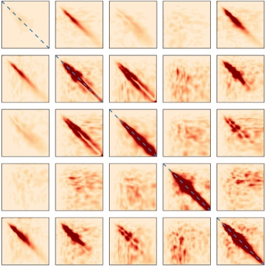
Figure 1. (a,b) Ensemble-averaged correlation tensor
 $\langle \,\hat {\!\boldsymbol q}^{{\prime \prime }}\,\hat {\!\boldsymbol q}^{{{\prime \prime }}{{H}}} \rangle$
(logarithmic scale to display all structures) from (a) the DNS data and (b) the eLNS model using the DNS-computed forcing, at
$\langle \,\hat {\!\boldsymbol q}^{{\prime \prime }}\,\hat {\!\boldsymbol q}^{{{\prime \prime }}{{H}}} \rangle$
(logarithmic scale to display all structures) from (a) the DNS data and (b) the eLNS model using the DNS-computed forcing, at
 $(k_x,k_z)h=(0.5,3)$
for case Ma15Re3k; only 15 components of the correlations out of 25 are shown because the tensor is Hermitian. (c–e) Leading eigenvalues of the correlation from DNS and the LNS/eLNS models using the DNS-computed forcing with
$(k_x,k_z)h=(0.5,3)$
for case Ma15Re3k; only 15 components of the correlations out of 25 are shown because the tensor is Hermitian. (c–e) Leading eigenvalues of the correlation from DNS and the LNS/eLNS models using the DNS-computed forcing with
 $(k_x,k_z)h$
equal to (c) (0.5, 3), (d) (3.5, 1) and (e) (20, 40).
$(k_x,k_z)h$
equal to (c) (0.5, 3), (d) (3.5, 1) and (e) (20, 40).
First, we inspect the mean-flow budgets in (2.1) for all the cases (shown in Appendix B). A term balance is realised throughout the field for each case, demonstrating the reliability of the averaged DNS data and the post-processing schemes. Second, we calculate the real forcing matrices
 $(\boldsymbol{{FF}}^{{H}})_{\textit{DNS}}$
and
$(\boldsymbol{{FF}}^{{H}})_{\textit{DNS}}$
and
 $(\boldsymbol{{EE}}^{{H}})_{\textit{DNS}}$
in (2.19) at different
$(\boldsymbol{{EE}}^{{H}})_{\textit{DNS}}$
in (2.19) at different
 $k_x$
,
$k_x$
,
 $k_z$
, and input them into the LNS and eLNS models in (2.14). Both models are anticipated to output
$k_z$
, and input them into the LNS and eLNS models in (2.14). Both models are anticipated to output
 $\widehat {\boldsymbol{\Phi }}$
values that are identical to
$\widehat {\boldsymbol{\Phi }}$
values that are identical to
 $\widehat {\boldsymbol{\Phi }}_{\textit{DNS}}$
. This is realised in figure 1 at nearly all
$\widehat {\boldsymbol{\Phi }}_{\textit{DNS}}$
. This is realised in figure 1 at nearly all
 $k_x$
and
$k_x$
and
 $k_z$
that are resolved. Specifically, close resemblance among
$k_z$
that are resolved. Specifically, close resemblance among
 $\widehat {\boldsymbol{\Phi }}_{\textit{LNS}}$
,
$\widehat {\boldsymbol{\Phi }}_{\textit{LNS}}$
,
 $\widehat {\boldsymbol{\Phi }}_{{e\kern-1pt L\kern-1pt N\kern-1pt S}}$
and
$\widehat {\boldsymbol{\Phi }}_{{e\kern-1pt L\kern-1pt N\kern-1pt S}}$
and
 $\widehat {\boldsymbol{\Phi }}_{\textit{DNS}}$
is observed in figures 1(a) and 1(b) for all the 15 components of
$\widehat {\boldsymbol{\Phi }}_{\textit{DNS}}$
is observed in figures 1(a) and 1(b) for all the 15 components of
 $\widehat {\boldsymbol{\Phi }}$
(hence
$\widehat {\boldsymbol{\Phi }}$
(hence
 $\widehat {\boldsymbol{\Phi }}_{\textit{LNS}}$
is not displayed for conciseness), at
$\widehat {\boldsymbol{\Phi }}_{\textit{LNS}}$
is not displayed for conciseness), at
 $(k_x,k_z)h=(0.5,3)$
(wavelengths
$(k_x,k_z)h=(0.5,3)$
(wavelengths
 $\lambda _x^+=2750,\lambda _z^+=460$
). A more quantitative comparison is shown in figure 1(c) by plotting the leading fortieth
$\lambda _x^+=2750,\lambda _z^+=460$
). A more quantitative comparison is shown in figure 1(c) by plotting the leading fortieth
 $\theta _j$
of the POD modes. They cover nearly four orders of magnitude, and the three sets of
$\theta _j$
of the POD modes. They cover nearly four orders of magnitude, and the three sets of
 $\theta _j$
are still in close agreement with each other. Such agreement in
$\theta _j$
are still in close agreement with each other. Such agreement in
 $\theta _j$
is also achieved at other
$\theta _j$
is also achieved at other
 $k_x$
and
$k_x$
and
 $k_z$
. Two representative results are displayed in figures 1(d) and 1(e), where
$k_z$
. Two representative results are displayed in figures 1(d) and 1(e), where
 $\lambda _x^+\lt \lambda _z^+$
for the former scale and
$\lambda _x^+\lt \lambda _z^+$
for the former scale and
 $\lambda _x^+,\lambda _z^+$
are both small (
$\lambda _x^+,\lambda _z^+$
are both small (
 ${\lt } 70$
) for the latter. The
${\lt } 70$
) for the latter. The
 $\theta _j$
from the eLNS model matches slightly better the DNS than the LNS model for different scales, and the reason will be clear in § 4.1.
$\theta _j$
from the eLNS model matches slightly better the DNS than the LNS model for different scales, and the reason will be clear in § 4.1.
Consequently, we arrive at the following two points. First, the value of
 $N_t$
in table 2 is adequate to obtain converged ensemble averages of the variables and nonlinear forcing at different scales. The computation of the complicated fluctuation terms in (2.3) is also accurate enough. Second, the framework of the stochastic linear models in § 2 is mathematically self-consistent. Both the LNS and eLNS models can provide accurate
$N_t$
in table 2 is adequate to obtain converged ensemble averages of the variables and nonlinear forcing at different scales. The computation of the complicated fluctuation terms in (2.3) is also accurate enough. Second, the framework of the stochastic linear models in § 2 is mathematically self-consistent. Both the LNS and eLNS models can provide accurate
 $\widehat {\boldsymbol{\Phi }}$
at different
$\widehat {\boldsymbol{\Phi }}$
at different
 $k_x$
and
$k_x$
and
 $k_z$
, if the forcings
$k_z$
, if the forcings
 $\boldsymbol{{FF}}^{{H}}$
and
$\boldsymbol{{FF}}^{{H}}$
and
 $\boldsymbol{{EE}}^{{H}}$
are accurate enough. In that case, the derived variables of
$\boldsymbol{{EE}}^{{H}}$
are accurate enough. In that case, the derived variables of
 $\widehat {\boldsymbol{\Phi }}$
, like the fluctuation variance, spatial spectra and the linear stochastic estimations (e.g. Madhusudanan et al. Reference Madhusudanan, Illingworth and Marusic2019), can also closely agree with DNS.
$\widehat {\boldsymbol{\Phi }}$
, like the fluctuation variance, spatial spectra and the linear stochastic estimations (e.g. Madhusudanan et al. Reference Madhusudanan, Illingworth and Marusic2019), can also closely agree with DNS.
4. Real forcing distributions from DNS
The characteristics of the real matrices
 $(\boldsymbol{{FF}}^{{H}})_{\textit{DNS}}$
and
$(\boldsymbol{{FF}}^{{H}})_{\textit{DNS}}$
and
 $(\boldsymbol{{EE}}^{{H}})_{\textit{DNS}}$
are detailed here. Prior to that, the nonlinear terms
$(\boldsymbol{{EE}}^{{H}})_{\textit{DNS}}$
are detailed here. Prior to that, the nonlinear terms
 ${\boldsymbol f}_q^{{\prime \prime }}$
and
${\boldsymbol f}_q^{{\prime \prime }}$
and
 ${\boldsymbol e}_q^{{\prime \prime }}$
from the DNS, required by
${\boldsymbol e}_q^{{\prime \prime }}$
from the DNS, required by
 $(\boldsymbol{{FF}}^{{H}})_{\textit{DNS}}$
and
$(\boldsymbol{{FF}}^{{H}})_{\textit{DNS}}$
and
 $(\boldsymbol{{EE}}^{{H}})_{\textit{DNS}}$
(see (2.19)), are discussed in § 4.1. Note that we concern with three central problems. The first is to clarify the relative contributions of different nonlinear components in (2.3) and table 1. The second is to examine whether the diagonally modelled forcing (2.15) aligns with the DNS statistics, which directly explains the success or failure of current models. The third is to reveal the differences between the LNS and eLNS models, and clarify the role of the critical eddy-viscosity-related terms.
$(\boldsymbol{{EE}}^{{H}})_{\textit{DNS}}$
(see (2.19)), are discussed in § 4.1. Note that we concern with three central problems. The first is to clarify the relative contributions of different nonlinear components in (2.3) and table 1. The second is to examine whether the diagonally modelled forcing (2.15) aligns with the DNS statistics, which directly explains the success or failure of current models. The third is to reveal the differences between the LNS and eLNS models, and clarify the role of the critical eddy-viscosity-related terms.

Figure 2. Root mean squares of different nonlinear fluctuation terms from DNS in the (a) streamwise, (b) wall-normal and (c) spanwise momentum equations, and (d) the enthalpy equation, for case Ma15Re3k. Panels (a–c) are normalised by
 $u_\tau$
and panel (d) is by
$u_\tau$
and panel (d) is by
 $T_\tau$
. See table 1 for term abbreviations. Note that all the components have been scaled by the mean-flow coefficients in (2.5b
), as in (2.6).
$T_\tau$
. See table 1 for term abbreviations. Note that all the components have been scaled by the mean-flow coefficients in (2.5b
), as in (2.6).

4.1. Distributions of the nonlinear terms
Given the significance of accurately computing the forcing (§ 3), we scrutinise each nonlinear fluctuation term defined in (2.3). Their root mean squares in the LNS and eLNS models are computed from the DNS. The wall-normal distributions of these components are plotted in figures 2 and 3 for cases Ma15Re3k and Ma30Re5k, respectively. The LNS model is discussed first. For
 $f_{u,\textit {rms}}^{{\prime \prime }}$
and
$f_{u,\textit {rms}}^{{\prime \prime }}$
and
 $f_{T,\textit {rms}}^{{\prime \prime }}$
, RSF and THF are respectively the dominant terms in nearly all regions. The terms related to molecular viscosity and conductivity (VSNF, VDNF and MHNF) are negligible except in the viscous sublayer, and the pressure-related terms PGNF and PCNF remain small throughout. For
$f_{T,\textit {rms}}^{{\prime \prime }}$
, RSF and THF are respectively the dominant terms in nearly all regions. The terms related to molecular viscosity and conductivity (VSNF, VDNF and MHNF) are negligible except in the viscous sublayer, and the pressure-related terms PGNF and PCNF remain small throughout. For
 $f_{v,\textit {rms}}^{{\prime \prime }}$
and
$f_{v,\textit {rms}}^{{\prime \prime }}$
and
 $f_{w,\textit {rms}}^{{\prime \prime }}$
, RSF still dominates away from the wall, but within and below the buffer layer, PGNF is significant and leads to an additional peak of
$f_{w,\textit {rms}}^{{\prime \prime }}$
, RSF still dominates away from the wall, but within and below the buffer layer, PGNF is significant and leads to an additional peak of
 $f_{\textit {rms}}^{{\prime \prime }}$
, especially for case Ma30Re5k (figures 3
b and 3
c). Therefore, the compressibility effect is prominent near the wall for the nonlinear terms in the wall-normal and spanwise momentum equations. The physics behind this additional peak will be clarified later using its spectra. Moreover, the convection-related terms MMNF and EMNF remain moderate throughout the field. They become increasingly important as
$f_{\textit {rms}}^{{\prime \prime }}$
, especially for case Ma30Re5k (figures 3
b and 3
c). Therefore, the compressibility effect is prominent near the wall for the nonlinear terms in the wall-normal and spanwise momentum equations. The physics behind this additional peak will be clarified later using its spectra. Moreover, the convection-related terms MMNF and EMNF remain moderate throughout the field. They become increasingly important as
 ${\textit {Ma}}_b$
rises, suggesting notable convection of momentum and energy caused by
${\textit {Ma}}_b$
rises, suggesting notable convection of momentum and energy caused by
 $\rho ^{\prime }$
. The results of case Ma15Re9k are qualitatively the same as case Ma15Re3k, and are hence not displayed.
$\rho ^{\prime }$
. The results of case Ma15Re9k are qualitatively the same as case Ma15Re3k, and are hence not displayed.
Next, we turn to the eLNS model. The original intention of introducing
 $\tau _R^{\prime }$
and
$\tau _R^{\prime }$
and
 $\vartheta _R^{\prime }$
is to partially model RSF and THF, so the residual terms eRSF and eTHF should be smaller than RSF and THF (see (2.8)). In figures 2 and 3, however, the results are the opposite. For all the equations shown, eRSF and eTHF are close to RSF and THF at
$\vartheta _R^{\prime }$
is to partially model RSF and THF, so the residual terms eRSF and eTHF should be smaller than RSF and THF (see (2.8)). In figures 2 and 3, however, the results are the opposite. For all the equations shown, eRSF and eTHF are close to RSF and THF at
 $y^*\lesssim 15$
, where
$y^*\lesssim 15$
, where
 $\mu _t/\,\bar {\!\mu }$
(and
$\mu _t/\,\bar {\!\mu }$
(and
 $\kappa _t/\bar {\kappa }$
) is small. In the outer region with
$\kappa _t/\bar {\kappa }$
) is small. In the outer region with
 $\mu _t\gg \,\bar {\!\mu }$
, however, eRSF and eTHF can be over two times larger than RSF and THF, so
$\mu _t\gg \,\bar {\!\mu }$
, however, eRSF and eTHF can be over two times larger than RSF and THF, so
 $e_{\textit {rms}}^{{\prime \prime }}$
are much higher than
$e_{\textit {rms}}^{{\prime \prime }}$
are much higher than
 $f_{\textit {rms}}^{{\prime \prime }}$
in all the momentum and enthalpy equations. The
$f_{\textit {rms}}^{{\prime \prime }}$
in all the momentum and enthalpy equations. The
 $\textit{Re}_\tau$
in the present cases are relatively low, so the ratio
$\textit{Re}_\tau$
in the present cases are relatively low, so the ratio
 $e_{\textit {rms}}^{{\prime \prime }}/f_{\textit {rms}}^{{\prime \prime }}$
will become even larger under higher
$e_{\textit {rms}}^{{\prime \prime }}/f_{\textit {rms}}^{{\prime \prime }}$
will become even larger under higher
 $\textit{Re}_\tau$
, due to the increased
$\textit{Re}_\tau$
, due to the increased
 $\mu _t/\,\bar {\!\mu }$
.
$\mu _t/\,\bar {\!\mu }$
.

Figure 4. Variance of the three terms in (2.8) and the correlation between RSF and the modelled stress flux (all normalised by
 $u_\tau ^2$
) for case Ma30Re5k: (a) streamwise and (b) wall-normal momentum equations.
$u_\tau ^2$
) for case Ma30Re5k: (a) streamwise and (b) wall-normal momentum equations.
Considering the unusual trend of eRSF and eTHF, the modelling assumption (2.8) deserves more discussion. The variances of the three components in (2.8), i.e.
 ${\textit{RSF}}_i$
,
${\textit{RSF}}_i$
,
 ${\partial \tau _{R,{i\!j}}^{\prime }}/{\partial x_j}$
and
${\partial \tau _{R,{i\!j}}^{\prime }}/{\partial x_j}$
and
 ${\textit{eRSF}}_i$
, are plotted in figure 4 for case Ma30Re5k, along with the correlation between
${\textit{eRSF}}_i$
, are plotted in figure 4 for case Ma30Re5k, along with the correlation between
 ${\textit{RSF}}_i$
and
${\textit{RSF}}_i$
and
 ${\partial \tau _{R,{i\!j}}^{\prime }}/{\partial x_j}$
. For both the streamwise and wall-normal momentum equations (and also the spanwise one not shown), the modelled stress flux
${\partial \tau _{R,{i\!j}}^{\prime }}/{\partial x_j}$
. For both the streamwise and wall-normal momentum equations (and also the spanwise one not shown), the modelled stress flux
 ${\partial \tau _{R,{i\!j}}^{\prime }}/{\partial x_j}$
does not follow
${\partial \tau _{R,{i\!j}}^{\prime }}/{\partial x_j}$
does not follow
 ${\textit{RSF}}_i$
throughout, regarding both shapes and amplitudes. The modelled flux highly overestimates, and has moderately negative correction with RSF in the outer layer, which leads to the much higher amplitudes of eRSF and RSF. The same conclusion applies to THF and eTHF. Also, we have examined that the trends in figure 4 are analogous for other cases, insensitive to
${\textit{RSF}}_i$
throughout, regarding both shapes and amplitudes. The modelled flux highly overestimates, and has moderately negative correction with RSF in the outer layer, which leads to the much higher amplitudes of eRSF and RSF. The same conclusion applies to THF and eTHF. Also, we have examined that the trends in figure 4 are analogous for other cases, insensitive to
 $\textit{Re}_\tau$
and
$\textit{Re}_\tau$
and
 ${\textit {Ma}}_b$
.
${\textit {Ma}}_b$
.
Consequently, we arrive at a conclusion that, the
 $\tau _R^{\prime }$
and
$\tau _R^{\prime }$
and
 $\vartheta _R^{\prime }$
fluxes are not partial modellings of RSF and THF, as previously believed (Hwang & Cossu Reference Hwang and Cossu2010; Pickering et al. Reference Pickering, Rigas, Schmidt, Sipp and Colonius2021; Chen et al. Reference Chen, Cheng, Fu and Gan2023a
; Ying et al. Reference Ying, Liang, Li and Fu2023). On the contrary, the ‘residual’ terms eRSF and eTHF can be several times larger than RSF and THF, so
$\vartheta _R^{\prime }$
fluxes are not partial modellings of RSF and THF, as previously believed (Hwang & Cossu Reference Hwang and Cossu2010; Pickering et al. Reference Pickering, Rigas, Schmidt, Sipp and Colonius2021; Chen et al. Reference Chen, Cheng, Fu and Gan2023a
; Ying et al. Reference Ying, Liang, Li and Fu2023). On the contrary, the ‘residual’ terms eRSF and eTHF can be several times larger than RSF and THF, so
 $e_{\textit {rms}}^{{\prime \prime }}$
is more dominant by eRSF and eTHF, than the dominance of RSF and THF over
$e_{\textit {rms}}^{{\prime \prime }}$
is more dominant by eRSF and eTHF, than the dominance of RSF and THF over
 $f_{\textit {rms}}^{{\prime \prime }}$
. As a result, the effects of other unmodelled nonlinear fluctuations (VSNF, MMNF, etc.) become minor, which increases the robustness of the shapes and amplitudes of the forcing. More discussions on this point will be provided in § 4.2. This robustness of the eLNS forcing also explains the trend in figure 1 that its ensemble average can reach convergence using a lower
$f_{\textit {rms}}^{{\prime \prime }}$
. As a result, the effects of other unmodelled nonlinear fluctuations (VSNF, MMNF, etc.) become minor, which increases the robustness of the shapes and amplitudes of the forcing. More discussions on this point will be provided in § 4.2. This robustness of the eLNS forcing also explains the trend in figure 1 that its ensemble average can reach convergence using a lower
 $N_t$
than the LNS counterpart.
$N_t$
than the LNS counterpart.
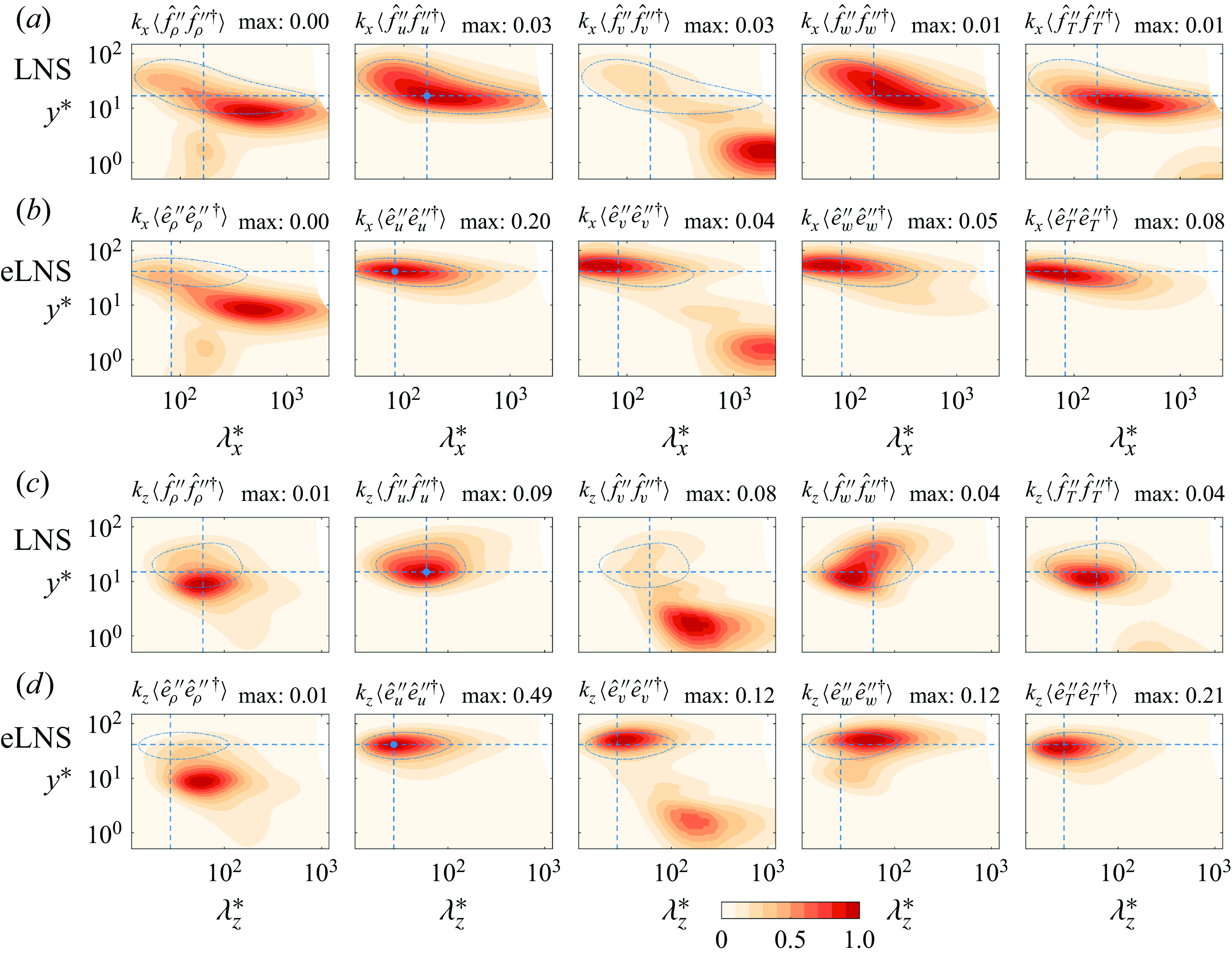
Figure 5. Pre-multiplied one-dimensional spectra of the nonlinear fluctuation terms in the (a,b) streamwise and (c,d) spanwise directions in semi-local units, for the (a,c) LNS model (
 $\,\hat {\!\boldsymbol f}_q^{{\prime \prime }}$
) and (b, d) eLNS model (
$\,\hat {\!\boldsymbol f}_q^{{\prime \prime }}$
) and (b, d) eLNS model (
 $\,\hat {\!\boldsymbol e}_q^{{\prime \prime }}$
), respectively, for case Ma30Re5k. The contours in each panel are normalised by their extreme values labelled on the top (in wall units
$\,\hat {\!\boldsymbol e}_q^{{\prime \prime }}$
), respectively, for case Ma30Re5k. The contours in each panel are normalised by their extreme values labelled on the top (in wall units
 $\rho _\tau$
,
$\rho _\tau$
,
 $u_\tau$
and
$u_\tau$
and
 $T_\tau$
). The blue dotted lines denote the peak location of the
$T_\tau$
). The blue dotted lines denote the peak location of the
 $u$
-spectrum, and the blue dashed lines denote the
$u$
-spectrum, and the blue dashed lines denote the
 $u$
-contour of 0.4.
$u$
-contour of 0.4.
The spectra of these nonlinear fluctuations are calculated, to identify the active wavenumbers of different components. Case Ma30Re5k is studied first, as it features the strongest density and temperature fluctuations. The pre-multiplied one-dimensional (1-D) spectra of
 $\,\hat {\!\boldsymbol f}_q^{{\prime \prime }}$
and
$\,\hat {\!\boldsymbol f}_q^{{\prime \prime }}$
and
 $\,\hat {\!\boldsymbol e}_q^{{\prime \prime }}$
in the streamwise and spanwise directions are displayed in figure 5. The semi-local coordinates
$\,\hat {\!\boldsymbol e}_q^{{\prime \prime }}$
in the streamwise and spanwise directions are displayed in figure 5. The semi-local coordinates
 $y^*$
,
$y^*$
,
 $\lambda _x^*$
and
$\lambda _x^*$
and
 $\lambda _z^*$
are adopted, and the spectra of the
$\lambda _z^*$
are adopted, and the spectra of the
 $u$
component are used as references in each row to examine the spectral similarity among different variables. A notable observation is that, compared with the LNS model, the spectra of
$u$
component are used as references in each row to examine the spectral similarity among different variables. A notable observation is that, compared with the LNS model, the spectra of
 $\,\hat {\!\boldsymbol e}_u^{{\prime \prime }}$
,
$\,\hat {\!\boldsymbol e}_u^{{\prime \prime }}$
,
 $\,\hat {\!\boldsymbol e}_v^{{\prime \prime }}$
,
$\,\hat {\!\boldsymbol e}_v^{{\prime \prime }}$
,
 $\,\hat {\!\boldsymbol e}_w^{{\prime \prime }}$
and
$\,\hat {\!\boldsymbol e}_w^{{\prime \prime }}$
and
 $\,\hat {\!\boldsymbol e}_T^{{\prime \prime }}$
in eLNS have greater resemblance to each other in shapes and peak locations for both the streamwise and spanwise ones; see figures 5(b) and 5(d). This similarity among variables can be explained by the dominance of eRSF and eTHF over other terms, as observed in figure 3. A further decomposition of
$\,\hat {\!\boldsymbol e}_T^{{\prime \prime }}$
in eLNS have greater resemblance to each other in shapes and peak locations for both the streamwise and spanwise ones; see figures 5(b) and 5(d). This similarity among variables can be explained by the dominance of eRSF and eTHF over other terms, as observed in figure 3. A further decomposition of
 $\partial \tau _{R,{i\!j}}^{\prime }/\partial x_j$
and
$\partial \tau _{R,{i\!j}}^{\prime }/\partial x_j$
and
 $\partial \vartheta _{R,j}^{\prime }/\partial x_j$
(difference between
$\partial \vartheta _{R,j}^{\prime }/\partial x_j$
(difference between
 ${\boldsymbol f}_q^{{\prime \prime }}$
and
${\boldsymbol f}_q^{{\prime \prime }}$
and
 ${\boldsymbol e}_q^{{\prime \prime }}$
) shows that the dominant terms for the four terms are
${\boldsymbol e}_q^{{\prime \prime }}$
) shows that the dominant terms for the four terms are
 $\mu _t \Delta \hat {u}^{{\prime \prime }}$
,
$\mu _t \Delta \hat {u}^{{\prime \prime }}$
,
 $\mu _t \Delta \hat {v}^{{\prime \prime }}$
,
$\mu _t \Delta \hat {v}^{{\prime \prime }}$
,
 $\mu _t \Delta \hat {w}^{{\prime \prime }}$
and
$\mu _t \Delta \hat {w}^{{\prime \prime }}$
and
 $\kappa _t \Delta \hat {T}^{{\prime \prime }}$
, respectively, with
$\kappa _t \Delta \hat {T}^{{\prime \prime }}$
, respectively, with
 $\Delta$
the Laplace operator. Therefore,
$\Delta$
the Laplace operator. Therefore,
 $\,\hat {\!\boldsymbol e}_q^{{\prime \prime }}$
resides in smaller scales than
$\,\hat {\!\boldsymbol e}_q^{{\prime \prime }}$
resides in smaller scales than
 $\hat {\boldsymbol q}^{{\kern0.3pt}{\prime \prime }}$
and
$\hat {\boldsymbol q}^{{\kern0.3pt}{\prime \prime }}$
and
 $\,\hat {\!\boldsymbol f}_q^{{\prime \prime }}$
, and the similarity among
$\,\hat {\!\boldsymbol f}_q^{{\prime \prime }}$
, and the similarity among
 $\,\hat {\!\boldsymbol e}_u^{{\prime \prime }}$
,
$\,\hat {\!\boldsymbol e}_u^{{\prime \prime }}$
,
 $\,\hat {\!\boldsymbol e}_v^{{\prime \prime }}$
,
$\,\hat {\!\boldsymbol e}_v^{{\prime \prime }}$
,
 $\,\hat {\!\boldsymbol e}_w^{{\prime \prime }}$
and
$\,\hat {\!\boldsymbol e}_w^{{\prime \prime }}$
and
 $\,\hat {\!\boldsymbol e}_T^{{\prime \prime }}$
is more easily established than
$\,\hat {\!\boldsymbol e}_T^{{\prime \prime }}$
is more easily established than
 $\,\hat {\!\boldsymbol f}^{{\prime \prime }}$
.
$\,\hat {\!\boldsymbol f}^{{\prime \prime }}$
.
An additional peak appears in the
 $\hat {f}_v^{{\prime \prime }}$
and
$\hat {f}_v^{{\prime \prime }}$
and
 $\hat {e}_v^{{\prime \prime }}$
spectra in the viscous sublayer, which is contributed by PGNF (equal to
$\hat {e}_v^{{\prime \prime }}$
spectra in the viscous sublayer, which is contributed by PGNF (equal to
 $-\partial (\rho ^{\prime } T^{{\prime \prime }})/\partial y$
) from figure 3. Compared with the outer peak, this inner peak resides in a larger scale of
$-\partial (\rho ^{\prime } T^{{\prime \prime }})/\partial y$
) from figure 3. Compared with the outer peak, this inner peak resides in a larger scale of
 $\lambda _z^*\approx 180$
. The value of
$\lambda _z^*\approx 180$
. The value of
 $\lambda _x^*$
of this inner peak exceeds 1500, but due to the relatively low
$\lambda _x^*$
of this inner peak exceeds 1500, but due to the relatively low
 $\textit{Re}_\tau$
in this case, its streamwise spectrum is not fully resolved. The
$\textit{Re}_\tau$
in this case, its streamwise spectrum is not fully resolved. The
 $\lambda _x^*\ll \lambda _z^*$
feature of this inner peak indicates that it is not caused by the near-wall acoustic motions (where
$\lambda _x^*\ll \lambda _z^*$
feature of this inner peak indicates that it is not caused by the near-wall acoustic motions (where
 $\lambda _x\lt \lambda _z$
; see § 5), but is attributed to the near-wall density and temperature streaks which are most active at
$\lambda _x\lt \lambda _z$
; see § 5), but is attributed to the near-wall density and temperature streaks which are most active at
 $\lambda _x^+\sim 1000$
and
$\lambda _x^+\sim 1000$
and
 $\lambda _z^+\sim 100$
; these two streaks are also in nearly perfect negative correlation (Coleman, Kim & Moser Reference Coleman, Kim and Moser1995; Patel, Boersma & Pecnik Reference Patel, Boersma and Pecnik2016; Cheng & Fu Reference Cheng and Fu2024).
$\lambda _z^+\sim 100$
; these two streaks are also in nearly perfect negative correlation (Coleman, Kim & Moser Reference Coleman, Kim and Moser1995; Patel, Boersma & Pecnik Reference Patel, Boersma and Pecnik2016; Cheng & Fu Reference Cheng and Fu2024).

Figure 6. Same as figure 5, but for (a,b) case Ma15Re3k and (c,d) case Ma15Re9k and only the results of the eLNS model are shown. Panels (a,c) are the streamwise spectra and panels (b,d) are the spanwise ones.
To examine the robustness of the spectral features of the eLNS nonlinear terms at different
 ${\textit {Ma}}_b$
and
${\textit {Ma}}_b$
and
 $\textit{Re}_\tau$
, the
1-D
spectra of
$\textit{Re}_\tau$
, the
1-D
spectra of
 $\,\hat {\!\boldsymbol e}_q^{{\prime \prime }}$
for cases Ma15Re3k and Ma15Re9k are depicted in figure 6. As in case Ma30Re5k, similarity between the spectra of
$\,\hat {\!\boldsymbol e}_q^{{\prime \prime }}$
for cases Ma15Re3k and Ma15Re9k are depicted in figure 6. As in case Ma30Re5k, similarity between the spectra of
 $\,\hat {\!\boldsymbol e}_u^{{\prime \prime }}$
,
$\,\hat {\!\boldsymbol e}_u^{{\prime \prime }}$
,
 $\,\hat {\!\boldsymbol e}_v^{{\prime \prime }}$
,
$\,\hat {\!\boldsymbol e}_v^{{\prime \prime }}$
,
 $\,\hat {\!\boldsymbol e}_w^{{\prime \prime }}$
and
$\,\hat {\!\boldsymbol e}_w^{{\prime \prime }}$
and
 $\,\hat {\!\boldsymbol e}_T^{{\prime \prime }}$
is observed in both the streamwise and spanwise directions. Meanwhile, the inner peak of
$\,\hat {\!\boldsymbol e}_T^{{\prime \prime }}$
is observed in both the streamwise and spanwise directions. Meanwhile, the inner peak of
 $\,\hat {\!\boldsymbol e}_v^{{\prime \prime }}$
due to the PGNF is less evident than in figure 5 owing to the reduced
$\,\hat {\!\boldsymbol e}_v^{{\prime \prime }}$
due to the PGNF is less evident than in figure 5 owing to the reduced
 ${\textit {Ma}}_b$
. Comparing between figures 6 and 5, we note that the (outer) peak location of these 1-D spectra is not sensitive to
${\textit {Ma}}_b$
. Comparing between figures 6 and 5, we note that the (outer) peak location of these 1-D spectra is not sensitive to
 ${\textit {Ma}}_b$
and
${\textit {Ma}}_b$
and
 $\textit{Re}_\tau$
after using the semi-local units, which is measured to be
$\textit{Re}_\tau$
after using the semi-local units, which is measured to be
 $\lambda _x^*\approx 90$
,
$\lambda _x^*\approx 90$
,
 $\lambda _x^*\approx 30$
and
$\lambda _x^*\approx 30$
and
 $y^*\approx 40$
.
$y^*\approx 40$
.
In short, we emphasise that the introduction of
 $\tau _R^{\prime }$
and
$\tau _R^{\prime }$
and
 $\vartheta _R^{\prime }$
is not a partial modelling of RSF and THF. On the contrary, it highly lifts the amplitudes of eRSF and eTHF, and hence the dominance of
$\vartheta _R^{\prime }$
is not a partial modelling of RSF and THF. On the contrary, it highly lifts the amplitudes of eRSF and eTHF, and hence the dominance of
 $\,\hat {\!\boldsymbol e}_q^{{\prime \prime }}$
by eRSF and eTHF. Therefore,
$\,\hat {\!\boldsymbol e}_q^{{\prime \prime }}$
by eRSF and eTHF. Therefore,
 $\,\hat {\!\boldsymbol e}_q^{{\prime \prime }}$
is more robust than
$\,\hat {\!\boldsymbol e}_q^{{\prime \prime }}$
is more robust than
 $\,\hat {\!\boldsymbol f}_q^{{\prime \prime }}$
for different variables in terms of the peaks and shapes of their physical and spectral distributions. Consequently,
$\,\hat {\!\boldsymbol f}_q^{{\prime \prime }}$
for different variables in terms of the peaks and shapes of their physical and spectral distributions. Consequently,
 $\,\hat {\!\boldsymbol e}_q^{{\prime \prime }}$
can be more easily modelled than
$\,\hat {\!\boldsymbol e}_q^{{\prime \prime }}$
can be more easily modelled than
 $\,\hat {\!\boldsymbol f}_q^{{\prime \prime }}$
by featuring more robust composition and structures, although this robustness may not always improve the model results; see § 4.2.
$\,\hat {\!\boldsymbol f}_q^{{\prime \prime }}$
by featuring more robust composition and structures, although this robustness may not always improve the model results; see § 4.2.
4.2. Distributions of the forcing matrix
As mentioned in § 3,
 $(\boldsymbol{{FF}}^{{H}})_{\textit{DNS}}$
and
$(\boldsymbol{{FF}}^{{H}})_{\textit{DNS}}$
and
 $(\boldsymbol{{EE}}^{{H}})_{\textit{DNS}}$
provide standard answers to how to model
$(\boldsymbol{{EE}}^{{H}})_{\textit{DNS}}$
provide standard answers to how to model
 $(\boldsymbol{{FF}}^{{H}})$
and
$(\boldsymbol{{FF}}^{{H}})$
and
 $(\boldsymbol{{EE}}^{{H}})$
in the stochastic linear models, so the distributions of these forcing are discussed at different
$(\boldsymbol{{EE}}^{{H}})$
in the stochastic linear models, so the distributions of these forcing are discussed at different
 $k_x$
and
$k_x$
and
 $k_z$
. The spectral fluctuation is usually classified into two branches according to its aspect ratio
$k_z$
. The spectral fluctuation is usually classified into two branches according to its aspect ratio
 $\lambda _x/\lambda _z$
. The structure with
$\lambda _x/\lambda _z$
. The structure with
 $\lambda _x\gt \lambda _z$
is considered as streamwise elongated, which is energetic and has strong linear coherence in the wall-normal direction (e.g. del Álamo & Jiménez Reference del Álamo and Jiménez2006). In comparison, the structure with
$\lambda _x\gt \lambda _z$
is considered as streamwise elongated, which is energetic and has strong linear coherence in the wall-normal direction (e.g. del Álamo & Jiménez Reference del Álamo and Jiménez2006). In comparison, the structure with
 $\lambda _x\lt \lambda _z$
is regarded as spanwise elongated, which receives energy from the nonlinear terms and can be worse predicted by the linear models than the streamwise-elongated one (Gupta et al. Reference Gupta, Madhusudanan, Wan, Illingworth and Juniper2021; Symon et al. Reference Symon, Illingworth and Marusic2021). These two types of fluctuations are discussed separately below.
$\lambda _x\lt \lambda _z$
is regarded as spanwise elongated, which receives energy from the nonlinear terms and can be worse predicted by the linear models than the streamwise-elongated one (Gupta et al. Reference Gupta, Madhusudanan, Wan, Illingworth and Juniper2021; Symon et al. Reference Symon, Illingworth and Marusic2021). These two types of fluctuations are discussed separately below.

Figure 7. Contours of the forcing matrix (a)
 $|(\boldsymbol{{FF}}^{{H}})_{\textit{DNS}}|$
and (b)
$|(\boldsymbol{{FF}}^{{H}})_{\textit{DNS}}|$
and (b)
 $|(\boldsymbol{{EE}}^{{H}})_{\textit{DNS}}|$
, at
$|(\boldsymbol{{EE}}^{{H}})_{\textit{DNS}}|$
, at
 $(k_x,k_z)h=(0.5,15)$
for case Ma30Re5k. Their diagonal terms, as labelled in blue dotted lines, are plotted in panels (c,d) in normalised values; the purple reference lines are from (2.15).
$(k_x,k_z)h=(0.5,15)$
for case Ma30Re5k. Their diagonal terms, as labelled in blue dotted lines, are plotted in panels (c,d) in normalised values; the purple reference lines are from (2.15).
The streamwise-elongated fluctuations are considered first. Figure 7 vividly demon- strates what the real forcing matrices
 $(\boldsymbol{{FF}}^{{H}})_{\textit{DNS}}$
and
$(\boldsymbol{{FF}}^{{H}})_{\textit{DNS}}$
and
 $(\boldsymbol{{EE}}^{{H}})_{\textit{DNS}}$
look like for case Ma30Re5k at
$(\boldsymbol{{EE}}^{{H}})_{\textit{DNS}}$
look like for case Ma30Re5k at
 $(k_x,k_z)h=(0.5,15)$
(
$(k_x,k_z)h=(0.5,15)$
(
 $\lambda _x=12.6h$
,
$\lambda _x=12.6h$
,
 $\lambda _z=0.4h$
). A direct observation is that these two matrices are far more complicated than the simple diagonal modelling in (2.15). Recall that two levels of simplification are made in (2.15). First, only the self-correlation matrices of the forcing variables (
$\lambda _z=0.4h$
). A direct observation is that these two matrices are far more complicated than the simple diagonal modelling in (2.15). Recall that two levels of simplification are made in (2.15). First, only the self-correlation matrices of the forcing variables (
 $\hat {f}_\rho ^{{\prime \prime }}\hat {f}_\rho ^{{{\prime \prime }}{{H}}}$
,
$\hat {f}_\rho ^{{\prime \prime }}\hat {f}_\rho ^{{{\prime \prime }}{{H}}}$
,
 $\hat {f}_u^{{\prime \prime }}\hat {f}_u^{{{\prime \prime }}{{H}}}$
, etc.) are retained, while all the inter-variable correlations (
$\hat {f}_u^{{\prime \prime }}\hat {f}_u^{{{\prime \prime }}{{H}}}$
, etc.) are retained, while all the inter-variable correlations (
 $\hat {f}_\rho ^{{\prime \prime }}\hat {f}_u^{{{\prime \prime }}{{H}}}$
, etc.) are neglected. Second, each self-correlation matrix is set to be diagonal, signifying perfect zero
correlation between different
$\hat {f}_\rho ^{{\prime \prime }}\hat {f}_u^{{{\prime \prime }}{{H}}}$
, etc.) are neglected. Second, each self-correlation matrix is set to be diagonal, signifying perfect zero
correlation between different
 $y$
. In figure 7, however, there are significant off-diagonal terms for both
$y$
. In figure 7, however, there are significant off-diagonal terms for both
 $(\boldsymbol{{FF}}^{{H}})_{\textit{DNS}}$
and
$(\boldsymbol{{FF}}^{{H}})_{\textit{DNS}}$
and
 $(\boldsymbol{{EE}}^{{H}})_{\textit{DNS}}$
, suggesting non-negligible inter-variable and inter-height correlations. Regarding the difference between the LNS and eLNS forcing, a visual observation seems to suggest that
$(\boldsymbol{{EE}}^{{H}})_{\textit{DNS}}$
, suggesting non-negligible inter-variable and inter-height correlations. Regarding the difference between the LNS and eLNS forcing, a visual observation seems to suggest that
 $(\boldsymbol{{EE}}^{{H}})_{\textit{DNS}}$
is more diagonal than
$(\boldsymbol{{EE}}^{{H}})_{\textit{DNS}}$
is more diagonal than
 $(\boldsymbol{{FF}}^{{H}})_{\textit{DNS}}$
, in terms of wall-normal correlations. This is reasonable because the dominant terms
$(\boldsymbol{{FF}}^{{H}})_{\textit{DNS}}$
, in terms of wall-normal correlations. This is reasonable because the dominant terms
 $\tau _R^{\prime }$
and
$\tau _R^{\prime }$
and
 $\vartheta _R^{\prime }$
in eLNS are linear functions of the fluctuations and are related to local mean-flow gradients, so they are more localised than the other nonlinear terms which contain high-order fluctuation moments. More quantitative evidence will be provided later. Consequently, the diagonal modelling in (2.15) benefits more the forcing in the eLNS model, than the LNS one. The diagonal elements of
$\vartheta _R^{\prime }$
in eLNS are linear functions of the fluctuations and are related to local mean-flow gradients, so they are more localised than the other nonlinear terms which contain high-order fluctuation moments. More quantitative evidence will be provided later. Consequently, the diagonal modelling in (2.15) benefits more the forcing in the eLNS model, than the LNS one. The diagonal elements of
 $(\boldsymbol{{FF}}^{{H}})_{\textit{DNS}}$
and
$(\boldsymbol{{FF}}^{{H}})_{\textit{DNS}}$
and
 $(\boldsymbol{{EE}}^{{H}})_{\textit{DNS}}$
are extracted in figures 7(c) and 7(d). The modelled distributions in (2.15) are also displayed for reference. As discussed in § 4.1, the diagonal terms for eLNS reflect the large contributions of eRSF and eTHF, so the diagonal terms of the
$(\boldsymbol{{EE}}^{{H}})_{\textit{DNS}}$
are extracted in figures 7(c) and 7(d). The modelled distributions in (2.15) are also displayed for reference. As discussed in § 4.1, the diagonal terms for eLNS reflect the large contributions of eRSF and eTHF, so the diagonal terms of the
 $u$
,
$u$
,
 $v$
,
$v$
,
 $w$
and
$w$
and
 $T$
components exhibit stronger resemblance to each other, hence they are more robust for modelling compared with the LNS model. Nevertheless, the prediction of (2.15) is not very consistent with the DNS results; the real forcing is more concentrated near the wall under this small
$T$
components exhibit stronger resemblance to each other, hence they are more robust for modelling compared with the LNS model. Nevertheless, the prediction of (2.15) is not very consistent with the DNS results; the real forcing is more concentrated near the wall under this small
 $\lambda _z$
.
$\lambda _z$
.
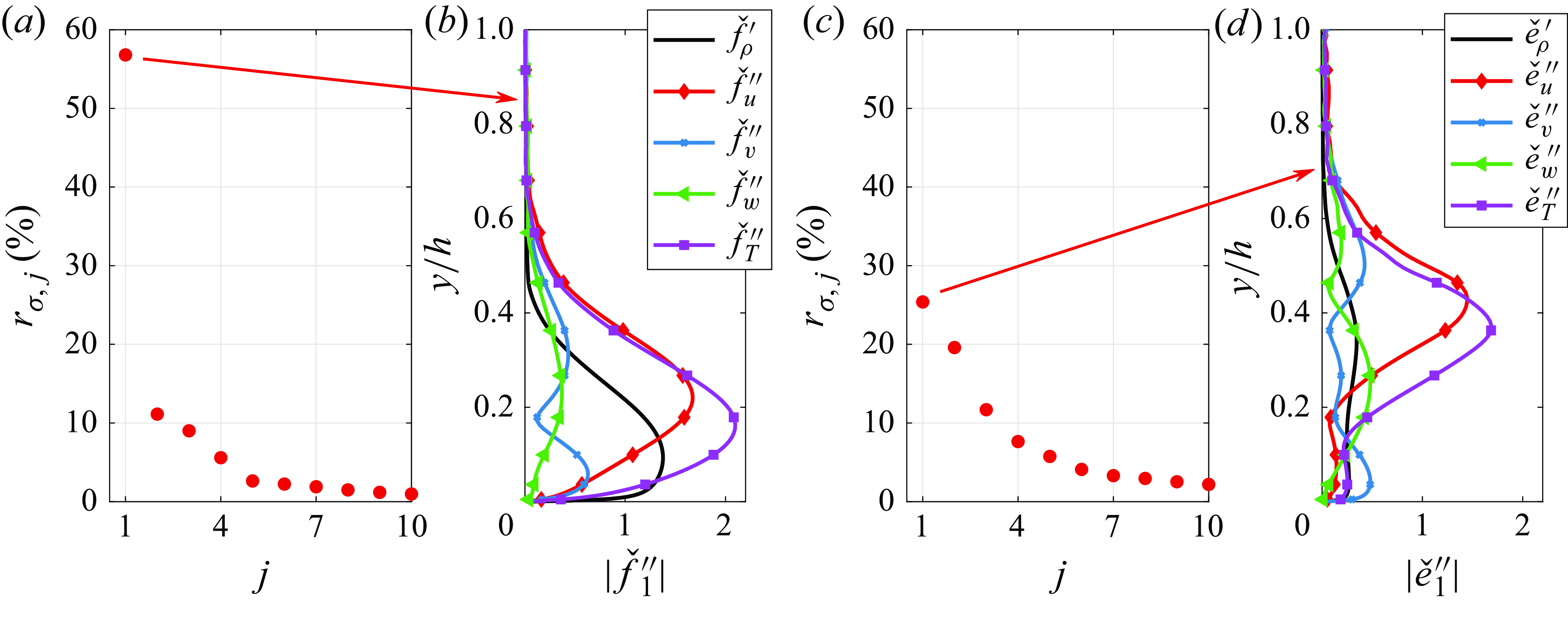
Figure 8. (a,c) Energy ratios occupied by the leading 10 singular values of the forcing matrix in figure 7, and (b,d) shape functions of the principal forcing mode (case Ma30Re5k,
 $(k_x,k_z)h=(0.5,15)$
). Panels (a,b) are for the LNS model, and (c,d) for the eLNS one.
$(k_x,k_z)h=(0.5,15)$
). Panels (a,b) are for the LNS model, and (c,d) for the eLNS one.
From the modelling perspective, it is interesting to show whether the DNS forcing is of low rank. The diagonal modelling in (2.15) means that the forcing is assumed to be of full rank, while Morra et al. (Reference Morra, Nogueira, Cavalieri and Henningson2021) demonstrate using the incompressible DNS data that the forcing has clear spatial-temporal coherence. The rank characteristics of the forcing matrix can be measured using the singular value decomposition (SVD), as
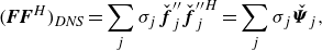 \begin{equation} (\boldsymbol{{FF}}^{{H}})_{\textit{DNS}} = \sum _j {\sigma _j \,\check {\!\boldsymbol f}_j^{{\prime \prime }} \,\check {\!\boldsymbol f}_j^{{{\prime \prime }}{{H}}}} = \sum _j { \sigma _j \,\check {\!\boldsymbol{\Psi }}_j }, \end{equation}
where
 $\sigma _j$
is the singular value sorted in the descending order;
$\sigma _j$
is the singular value sorted in the descending order;
 $\,\check {\!\boldsymbol f}_j^{{\prime \prime }}$
is the singular vector satisfying the orthogonal condition
$\,\check {\!\boldsymbol f}_j^{{\prime \prime }}$
is the singular vector satisfying the orthogonal condition
 $(\,\check {\!\boldsymbol f}_i^{{\prime \prime }},\,\check {\!\boldsymbol f}_j^{{\prime \prime }})_E=\delta _{{i\!j}}$
, so each component
$(\,\check {\!\boldsymbol f}_i^{{\prime \prime }},\,\check {\!\boldsymbol f}_j^{{\prime \prime }})_E=\delta _{{i\!j}}$
, so each component
 $\,\check {\!\boldsymbol{\Psi }}_j$
is of rank one. The left and right singular vectors are the same because the forcing matrix is Hermitian. Besides, the sum of the singular values,
$\,\check {\!\boldsymbol{\Psi }}_j$
is of rank one. The left and right singular vectors are the same because the forcing matrix is Hermitian. Besides, the sum of the singular values,
 $\sum _j{\sigma _j}\equiv V_\sigma$
, represents the total energy input by the forcing. The decomposition for
$\sum _j{\sigma _j}\equiv V_\sigma$
, represents the total energy input by the forcing. The decomposition for
 $(\boldsymbol{{EE}}^{{H}})_{\textit{DNS}}$
is defined likewise. Based on (4.1), we would regard a forcing matrix as of low rank if the first or first few SVD modes occupy a large portion of the total forcing energy.
$(\boldsymbol{{EE}}^{{H}})_{\textit{DNS}}$
is defined likewise. Based on (4.1), we would regard a forcing matrix as of low rank if the first or first few SVD modes occupy a large portion of the total forcing energy.
The leading ten
 $\sigma _{F,j}$
and
$\sigma _{F,j}$
and
 $\sigma _{E,j}$
of the matrices in figure 7 are plotted in figures 8(a) and 8(c), expressed in relative ratios
$\sigma _{E,j}$
of the matrices in figure 7 are plotted in figures 8(a) and 8(c), expressed in relative ratios
 $r_{\sigma ,j}=\sigma _j/V_\sigma$
. Note that
$r_{\sigma ,j}=\sigma _j/V_\sigma$
. Note that
 $\sigma _j$
appears in pairs due to the flow symmetry or antisymmetry on the two sides of the channel regarding the centreline, so every two
$\sigma _j$
appears in pairs due to the flow symmetry or antisymmetry on the two sides of the channel regarding the centreline, so every two
 $\sigma _j$
are combined to reflect their joint contributions. The forcing
$\sigma _j$
are combined to reflect their joint contributions. The forcing
 $(\boldsymbol{{FF}}^{{H}})_{\textit{DNS}}$
for the LNS model is of relatively low rank, with
$(\boldsymbol{{FF}}^{{H}})_{\textit{DNS}}$
for the LNS model is of relatively low rank, with
 $r_{\sigma F,1}$
over 57 %. This low-rank feature is very different from the full-rank
$r_{\sigma F,1}$
over 57 %. This low-rank feature is very different from the full-rank
 $\boldsymbol{{FF}}^{{H}}$
(fully diagonal) assumed in the linear model. The shape of the principal mode
$\boldsymbol{{FF}}^{{H}}$
(fully diagonal) assumed in the linear model. The shape of the principal mode
 $\,\check {\!\boldsymbol f}_1^{{\prime \prime }}$
is plotted in figure 8(b). The
$\,\check {\!\boldsymbol f}_1^{{\prime \prime }}$
is plotted in figure 8(b). The
 $\check {f}_{u,1}^{{\prime \prime }}$
and
$\check {f}_{u,1}^{{\prime \prime }}$
and
 $\check {f}_{T,1}^{{\prime \prime }}$
components turn out to be the two largest, which is different from a previous suggestion of the linear models that, for the principal forcing mode, the
$\check {f}_{T,1}^{{\prime \prime }}$
components turn out to be the two largest, which is different from a previous suggestion of the linear models that, for the principal forcing mode, the
 $\check {f}_{v,1}^{{\prime \prime }}$
and
$\check {f}_{v,1}^{{\prime \prime }}$
and
 $\check {f}_{w,1}^{{\prime \prime }}$
components are dominant for streamwise-elongated modes in the form of streamwise vortices to induce streaks (Hwang & Cossu Reference Hwang and Cossu2010; Chen et al. Reference Chen, Cheng, Fu and Gan2023a
). In comparison,
$\check {f}_{w,1}^{{\prime \prime }}$
components are dominant for streamwise-elongated modes in the form of streamwise vortices to induce streaks (Hwang & Cossu Reference Hwang and Cossu2010; Chen et al. Reference Chen, Cheng, Fu and Gan2023a
). In comparison,
 $r_{\sigma E,1}={26}\,\%$
for the eLNS model is lower than
$r_{\sigma E,1}={26}\,\%$
for the eLNS model is lower than
 $r_{\sigma F,1}$
. In other words, the modelled terms eRSF and eTHF lessen the spatial coherence of the forcing, and add to its diagonal dominance. Meanwhile, eRSF and eTHF markedly enhance the outer-layer forcing (figure 3), so the shapes of the principal mode in figure 8(d) is also lifted away from the wall, compared with its LNS counterpart. This amplified outer-layer forcing energy can be rapidly dissipated within the linear operator, where the stronger damping in eLNS is due to the replacement of
$r_{\sigma F,1}$
. In other words, the modelled terms eRSF and eTHF lessen the spatial coherence of the forcing, and add to its diagonal dominance. Meanwhile, eRSF and eTHF markedly enhance the outer-layer forcing (figure 3), so the shapes of the principal mode in figure 8(d) is also lifted away from the wall, compared with its LNS counterpart. This amplified outer-layer forcing energy can be rapidly dissipated within the linear operator, where the stronger damping in eLNS is due to the replacement of
 $\,\bar {\!\mu }$
with
$\,\bar {\!\mu }$
with
 $\,\bar {\!\mu }+\mu _t$
in the linear operator (see § 2.2). Consequently, the response mode can still take the form of near-wall streaky motions (c.f. figure 1
b also with
$\,\bar {\!\mu }+\mu _t$
in the linear operator (see § 2.2). Consequently, the response mode can still take the form of near-wall streaky motions (c.f. figure 1
b also with
 $\lambda _x\gt \lambda _z$
).
$\lambda _x\gt \lambda _z$
).

Figure 9. Same as figure 7 except for scale
 $(k_x,k_z)h=(20,3)$
.
$(k_x,k_z)h=(20,3)$
.
The forcing pattern for spanwise-elongated modes is demonstrated in figure 9, where the wavenumbers are selected to be
 $(k_x,k_z)h=(20,3)$
(
$(k_x,k_z)h=(20,3)$
(
 $\lambda _x=0.6h$
,
$\lambda _x=0.6h$
,
 $\lambda _z=4.2h$
). Compared with figure 7, the matrices
$\lambda _z=4.2h$
). Compared with figure 7, the matrices
 $(\boldsymbol{{FF}}^{{H}})_{\textit{DNS}}$
and
$(\boldsymbol{{FF}}^{{H}})_{\textit{DNS}}$
and
 $(\boldsymbol{{EE}}^{{H}})_{\textit{DNS}}$
become visually more diagonal in the wall-normal direction. Equivalently, the two forcings are both of higher rank, compared with those in figures 7, 8, which is inferred from their more uniform
$(\boldsymbol{{EE}}^{{H}})_{\textit{DNS}}$
become visually more diagonal in the wall-normal direction. Equivalently, the two forcings are both of higher rank, compared with those in figures 7, 8, which is inferred from their more uniform
 $\sigma _j$
(not shown;
$\sigma _j$
(not shown;
 $r_{\sigma F,1},r_{\sigma E,1}\lt {12}\,\%$
). This stronger diagonality for spanwise-elongated structures is reasonable, because they tend to be more localised and exhibit weak inter-layer linear coherence (e.g. Marusic, Baars & Hutchins Reference Marusic, Baars and Hutchins2017). The diagonal elements of the two forcing matrices are plotted in figures 9(c) and 9(d). It is interesting to show that the prediction of (2.15) is in good agreement with the DNS results, especially for the eLNS model. Nevertheless, both incompressible and compressible works suggest that the linear models perform worse for spanwise-elongated fluctuations (Gupta et al. Reference Gupta, Madhusudanan, Wan, Illingworth and Juniper2021; Symon et al. Reference Symon, Illingworth and Marusic2021; Chen et al. Reference Chen, Cheng, Gan and Fu2023b
). From the modelling aspect, a prominent disrupting factor is the unmodelled inter-variable correlations, particularly
$r_{\sigma F,1},r_{\sigma E,1}\lt {12}\,\%$
). This stronger diagonality for spanwise-elongated structures is reasonable, because they tend to be more localised and exhibit weak inter-layer linear coherence (e.g. Marusic, Baars & Hutchins Reference Marusic, Baars and Hutchins2017). The diagonal elements of the two forcing matrices are plotted in figures 9(c) and 9(d). It is interesting to show that the prediction of (2.15) is in good agreement with the DNS results, especially for the eLNS model. Nevertheless, both incompressible and compressible works suggest that the linear models perform worse for spanwise-elongated fluctuations (Gupta et al. Reference Gupta, Madhusudanan, Wan, Illingworth and Juniper2021; Symon et al. Reference Symon, Illingworth and Marusic2021; Chen et al. Reference Chen, Cheng, Gan and Fu2023b
). From the modelling aspect, a prominent disrupting factor is the unmodelled inter-variable correlations, particularly
 $\hat {f}_\rho ^{{\prime \prime }}\hat {f}_u^{{{\prime \prime }}{{H}}}$
,
$\hat {f}_\rho ^{{\prime \prime }}\hat {f}_u^{{{\prime \prime }}{{H}}}$
,
 $\hat {f}_\rho ^{{\prime \prime }}\hat {f}_T^{{{\prime \prime }}{{H}}}$
,
$\hat {f}_\rho ^{{\prime \prime }}\hat {f}_T^{{{\prime \prime }}{{H}}}$
,
 $\hat {f}_u^{{\prime \prime }}\hat {f}_v^{{{\prime \prime }}{{H}}}$
and
$\hat {f}_u^{{\prime \prime }}\hat {f}_v^{{{\prime \prime }}{{H}}}$
and
 $\hat {f}_u^{{\prime \prime }}\hat {f}_T^{{{\prime \prime }}{{H}}}$
(and also the
$\hat {f}_u^{{\prime \prime }}\hat {f}_T^{{{\prime \prime }}{{H}}}$
(and also the
 $\hat {e}^{{\prime \prime }}$
counterparts). They are all assumed zero in (2.15). From the physical perspective, previous studies showed that the linear dynamics (lift-up mechanism, transient growth, etc.) is important for generating streamwise-elongated structures, but contrarily, the travelling-wave-like spanwise-elongated fluctuations are mainly caused by nonlinear effects related to turbulent bursting, vortex stretching and streak breakdown (Schoppa & Hussain Reference Schoppa and Hussain2002; Yu et al. Reference Yu, Zhou, Dong, Yuan and Xu2024).
$\hat {e}^{{\prime \prime }}$
counterparts). They are all assumed zero in (2.15). From the physical perspective, previous studies showed that the linear dynamics (lift-up mechanism, transient growth, etc.) is important for generating streamwise-elongated structures, but contrarily, the travelling-wave-like spanwise-elongated fluctuations are mainly caused by nonlinear effects related to turbulent bursting, vortex stretching and streak breakdown (Schoppa & Hussain Reference Schoppa and Hussain2002; Yu et al. Reference Yu, Zhou, Dong, Yuan and Xu2024).

Figure 10. Projection coefficients of the DNS forcing to the space spanned by the POD modes for case Ma30Re5k: (a,b,c,d) LNS part
 $\alpha _{{i\!j}}$
, (e,f,g,h) eddy-viscosity part
$\alpha _{{i\!j}}$
, (e,f,g,h) eddy-viscosity part
 $\xi _{{i\!j}}$
and (i,j,k,l) eLNS part
$\xi _{{i\!j}}$
and (i,j,k,l) eLNS part
 $\beta _{{i\!j}}$
; see (4.2). Panels show (a,e,i)
$\beta _{{i\!j}}$
; see (4.2). Panels show (a,e,i)
 $\lambda _x=6.3h$
,
$\lambda _x=6.3h$
,
 $\lambda _z=3.1h$
; (b,f,j)
$\lambda _z=3.1h$
; (b,f,j)
 $\lambda _x=6.3h$
,
$\lambda _x=6.3h$
,
 $\lambda _z^+=179$
; (c,g,k)
$\lambda _z^+=179$
; (c,g,k)
 $\lambda _x^+=143$
,
$\lambda _x^+=143$
,
 $\lambda _z=3.1h$
; (d,h,l)
$\lambda _z=3.1h$
; (d,h,l)
 $\lambda _x^+=143$
,
$\lambda _x^+=143$
,
 $\lambda _z^+=179$
. The input energy
$\lambda _z^+=179$
. The input energy
 $V_\sigma$
shown is amplified by 105 for all panels for convenience.
$V_\sigma$
shown is amplified by 105 for all panels for convenience.
The diagonality of the forcing matrices in figures 7 and 9 relies on visual measurement. For more quantitative estimation, we project the forcing into the space spanned by the POD modes of
 $\langle \hat {\boldsymbol q}^{{\kern0.3pt}{\prime \prime }}\hat {\boldsymbol q}^{{{\prime \prime }}{{H}}} \rangle$
. The projection coefficients for models LNS and eLNS are then computed as
$\langle \hat {\boldsymbol q}^{{\kern0.3pt}{\prime \prime }}\hat {\boldsymbol q}^{{{\prime \prime }}{{H}}} \rangle$
. The projection coefficients for models LNS and eLNS are then computed as
 \begin{equation} \alpha _{{i\!j}} = \,\check {\!\boldsymbol q}_i^{{{\prime \prime }}{{H}}}\boldsymbol{M}\big(\boldsymbol{{FF}}^{{H}}\big)_{\textit{DNS}} \boldsymbol{M} \,\check {\!\boldsymbol q}_j^{{\prime \prime }}, \qquad \beta _{{i\!j}} = \,\check {\!\boldsymbol q}_i^{{{\prime \prime }}{{H}}}\boldsymbol{M}\big(\boldsymbol{{EE}}^{{H}}\big)_{\textit{DNS}} \boldsymbol{M} \,\check {\!\boldsymbol q}_j^{{\prime \prime }}. \end{equation}
This projection reduces the forcing in the physical space into discrete coefficients, and can jointly reflect inter-variable and inter-height correlations. If the forcing is ideally a white noise modelled by (2.15), then
 $\alpha _{{i\!j}}$
(and
$\alpha _{{i\!j}}$
(and
 $\beta _{{i\!j}}$
) is also a diagonally dominant matrix for nearly all spatial scales. The difference between
$\beta _{{i\!j}}$
) is also a diagonally dominant matrix for nearly all spatial scales. The difference between
 $\alpha _{{i\!j}}$
and
$\alpha _{{i\!j}}$
and
 $\beta _{{i\!j}}$
is also of interest, denoted as
$\beta _{{i\!j}}$
is also of interest, denoted as
 $\xi _{{i\!j}}=\beta _{{i\!j}}-\alpha _{{i\!j}}$
, which reflects the contribution of the eddy-viscosity-related terms.
$\xi _{{i\!j}}=\beta _{{i\!j}}-\alpha _{{i\!j}}$
, which reflects the contribution of the eddy-viscosity-related terms.
The Ma30Re5k case is discussed first using four representative scales. The first two are streamwise- and spanwise-elongated fluctuations discussed above; the third type is a large-scale fluctuation in the outer region with
 $(\lambda _x,\lambda _z)/h=(6.3,3.1)$
, and the fourth is a small-scale fluctuation with
$(\lambda _x,\lambda _z)/h=(6.3,3.1)$
, and the fourth is a small-scale fluctuation with
 $\lambda _x^+,\lambda _z^+\sim 100$
. Their
$\lambda _x^+,\lambda _z^+\sim 100$
. Their
 $\alpha _{{i\!j}}$
,
$\alpha _{{i\!j}}$
,
 $\xi _{{i\!j}}$
and
$\xi _{{i\!j}}$
and
 $\beta _{{i\!j}}$
values are depicted in figure 10 for the leading indices
$\beta _{{i\!j}}$
values are depicted in figure 10 for the leading indices
 $i,j\lt 10$
. These coefficients are normalised by their input energy
$i,j\lt 10$
. These coefficients are normalised by their input energy
 $V_{\sigma }$
, as labelled, such that their trace is unity:
$V_{\sigma }$
, as labelled, such that their trace is unity:
 $\Sigma _i \alpha _{ii}/V_{\sigma ,\alpha }=1$
(so are
$\Sigma _i \alpha _{ii}/V_{\sigma ,\alpha }=1$
(so are
 $\xi _{{i\!j}}$
and
$\xi _{{i\!j}}$
and
 $\beta _{{i\!j}}$
). For the large-scale fluctuation in figure 10(a),
$\beta _{{i\!j}}$
). For the large-scale fluctuation in figure 10(a),
 $\alpha _{{i\!j}}$
for the LNS model has pronounced off-diagonal elements, indicating strong inter-variable and/or inter-height correlations. In comparison, the eddy-viscosity term
$\alpha _{{i\!j}}$
for the LNS model has pronounced off-diagonal elements, indicating strong inter-variable and/or inter-height correlations. In comparison, the eddy-viscosity term
 $\xi _{{i\!j}}$
has much higher energy (
$\xi _{{i\!j}}$
has much higher energy (
 $V_\sigma$
) than
$V_\sigma$
) than
 $\alpha _{{i\!j}}$
, as discussed for figure 3, and is highly diagonally dominant. As a result, their summation
$\alpha _{{i\!j}}$
, as discussed for figure 3, and is highly diagonally dominant. As a result, their summation
 $\beta _{{i\!j}}=\alpha _{{i\!j}}+\xi _{{i\!j}}$
for the eLNS model has a similar distribution to
$\beta _{{i\!j}}=\alpha _{{i\!j}}+\xi _{{i\!j}}$
for the eLNS model has a similar distribution to
 $\xi _{{i\!j}}$
and features high diagonal dominance. The above trend is analogous to streamwise-elongated structures in the second column of figure 10, which has been visually shown in figure 9. In comparison, for the structures of small
$\xi _{{i\!j}}$
and features high diagonal dominance. The above trend is analogous to streamwise-elongated structures in the second column of figure 10, which has been visually shown in figure 9. In comparison, for the structures of small
 $\lambda _x$
(irrespective of
$\lambda _x$
(irrespective of
 $\lambda _z$
),
$\lambda _z$
),
 $\alpha _{{i\!j}}$
,
$\alpha _{{i\!j}}$
,
 $\xi _{{i\!j}}$
and
$\xi _{{i\!j}}$
and
 $\beta _{{i\!j}}$
are all diagonally dominant, as shown in the last two columns of figure 10, which is in line with the observations in figure 9.
$\beta _{{i\!j}}$
are all diagonally dominant, as shown in the last two columns of figure 10, which is in line with the observations in figure 9.

Figure 11. Same as figure 10 but for (a,b,e,f) case Ma15Re3k and (c,d,g,h) case Ma15Re9k. Panels (a,c,e,g) are fluctuations of large
 $\lambda _x$
,
$\lambda _x$
,
 $\lambda _z$
and panels (b,d,f,h) are of small
$\lambda _z$
and panels (b,d,f,h) are of small
 $\lambda _x$
,
$\lambda _x$
,
 $\lambda _z$
.
$\lambda _z$
.
The projection results for cases Ma15Re3k and Ma15Re9k are shown in figure 11. The distributions of
 $\alpha _{{i\!j}}$
and
$\alpha _{{i\!j}}$
and
 $\beta _{{i\!j}}$
for different scales resemble a lot those in figure 10, suggesting weak dependence on
$\beta _{{i\!j}}$
for different scales resemble a lot those in figure 10, suggesting weak dependence on
 ${\textit {Ma}}_b$
and
${\textit {Ma}}_b$
and
 $\textit{Re}_\tau$
. Therefore, the role of the eddy-viscosity terms is clarified again (as in § 4.1) that it adds a large-amplitude diagonally
dominant term to the LNS forcing matrix (specifically, the self-correlation part of the forcing variables), so that the eLNS forcing is more diagonally dominant and has similar shapes at different scales. From the physical point of view, this enhanced diagonal dominance was shown to build a better balance between local turbulent energy dissipation and transport (Symon et al. Reference Symon, Madhusudanan, Illingworth and Marusic2023; Ying et al. Reference Ying, Chen, Li and Fu2024a
). Consequently, the eLNS model is more robust among different scales in predicting variable correlations than LNS.
$\textit{Re}_\tau$
. Therefore, the role of the eddy-viscosity terms is clarified again (as in § 4.1) that it adds a large-amplitude diagonally
dominant term to the LNS forcing matrix (specifically, the self-correlation part of the forcing variables), so that the eLNS forcing is more diagonally dominant and has similar shapes at different scales. From the physical point of view, this enhanced diagonal dominance was shown to build a better balance between local turbulent energy dissipation and transport (Symon et al. Reference Symon, Madhusudanan, Illingworth and Marusic2023; Ying et al. Reference Ying, Chen, Li and Fu2024a
). Consequently, the eLNS model is more robust among different scales in predicting variable correlations than LNS.
Based on the above conclusion, a natural thought to improve the model arises that the robustness of the eLNS model can be further strengthened by artificially adding very large diagonal elements, for example, 10 times
 ${\rm{eRSF}}$
, although unphysical, to the forcing matrix
${\rm{eRSF}}$
, although unphysical, to the forcing matrix
 $(\boldsymbol{{EE}}^{{H}})$
. Nevertheless, we note that the model behaviours will not be necessarily improved for two reasons. First, although the inter-height correlation is more robustly modelled, the off-diagonal inter-variable correlation for the forcing also matters (see figure 9), so the relative amplitudes of different variables still need to be carefully determined. Second, artificial enhancement of the diagonal terms can destroy the non-normality of the NS operator, as already reflected in the eLNS model to some extent (Symon et al. Reference Symon, Illingworth and Marusic2021; Chen et al. Reference Chen, Cheng, Gan and Fu2023b
). As a result, not only can the linear amplification mechanism be disrupted, but also the energies of different branches of modes can be disorderly sorted, possibly leading to excessive amplification of the acoustic and other components for compressible flows.
$(\boldsymbol{{EE}}^{{H}})$
. Nevertheless, we note that the model behaviours will not be necessarily improved for two reasons. First, although the inter-height correlation is more robustly modelled, the off-diagonal inter-variable correlation for the forcing also matters (see figure 9), so the relative amplitudes of different variables still need to be carefully determined. Second, artificial enhancement of the diagonal terms can destroy the non-normality of the NS operator, as already reflected in the eLNS model to some extent (Symon et al. Reference Symon, Illingworth and Marusic2021; Chen et al. Reference Chen, Cheng, Gan and Fu2023b
). As a result, not only can the linear amplification mechanism be disrupted, but also the energies of different branches of modes can be disorderly sorted, possibly leading to excessive amplification of the acoustic and other components for compressible flows.
Finally, we provide a global view of the coherence of the LNS and eLNS forcing at all scales. The contours of
 $r_{\sigma ,1}$
, which measures the energy ratio of the most energetic forcing mode to all modes, are plotted in figure 12 for all three cases. For the LNS model, the forcing for streamwise-elongated fluctuations (
$r_{\sigma ,1}$
, which measures the energy ratio of the most energetic forcing mode to all modes, are plotted in figure 12 for all three cases. For the LNS model, the forcing for streamwise-elongated fluctuations (
 $\lambda _x\gt \lambda _z$
) has relatively high coherence and low rank, compared with the spanwise-elongated parts. The maximum
$\lambda _x\gt \lambda _z$
) has relatively high coherence and low rank, compared with the spanwise-elongated parts. The maximum
 $r_{\sigma ,1}$
for case Ma15Re3k reaches over 70 % at
$r_{\sigma ,1}$
for case Ma15Re3k reaches over 70 % at
 $(\lambda _x,\lambda _z)/h\approx (12.6,0.7)$
. The maxima in other two cases (figures 12
b and 12
c) also appear at approximately the same scale, suggesting a robust mechanism of scale selection for the forcing at different
$(\lambda _x,\lambda _z)/h\approx (12.6,0.7)$
. The maxima in other two cases (figures 12
b and 12
c) also appear at approximately the same scale, suggesting a robust mechanism of scale selection for the forcing at different
 ${\textit {Ma}}_b$
and
${\textit {Ma}}_b$
and
 $\textit{Re}_\tau$
. As discussed above, this low-rank feature of the LNS forcing at
$\textit{Re}_\tau$
. As discussed above, this low-rank feature of the LNS forcing at
 $\lambda _x\gt \lambda _z$
explains its poor behaviours in predicting these energetic fluctuations (e.g. Madhusudanan et al. Reference Madhusudanan, Illingworth and Marusic2019). Meanwhile, we notice that the distribution of
$\lambda _x\gt \lambda _z$
explains its poor behaviours in predicting these energetic fluctuations (e.g. Madhusudanan et al. Reference Madhusudanan, Illingworth and Marusic2019). Meanwhile, we notice that the distribution of
 $r_{\sigma ,1}$
resembles a lot the linear coherence spectra of
$r_{\sigma ,1}$
resembles a lot the linear coherence spectra of
 $u$
and
$u$
and
 $T$
between different heights (Marusic et al. Reference Marusic, Baars and Hutchins2017; Gupta et al. Reference Gupta, Madhusudanan, Wan, Illingworth and Juniper2021; Chen et al. Reference Chen, Cheng, Gan and Fu2023b
) within the inner–outer interaction model. Therefore, the LNS forcing for the scales with strong inter-height linear coherence of velocity and temperature is of particularly low rank.
$T$
between different heights (Marusic et al. Reference Marusic, Baars and Hutchins2017; Gupta et al. Reference Gupta, Madhusudanan, Wan, Illingworth and Juniper2021; Chen et al. Reference Chen, Cheng, Gan and Fu2023b
) within the inner–outer interaction model. Therefore, the LNS forcing for the scales with strong inter-height linear coherence of velocity and temperature is of particularly low rank.
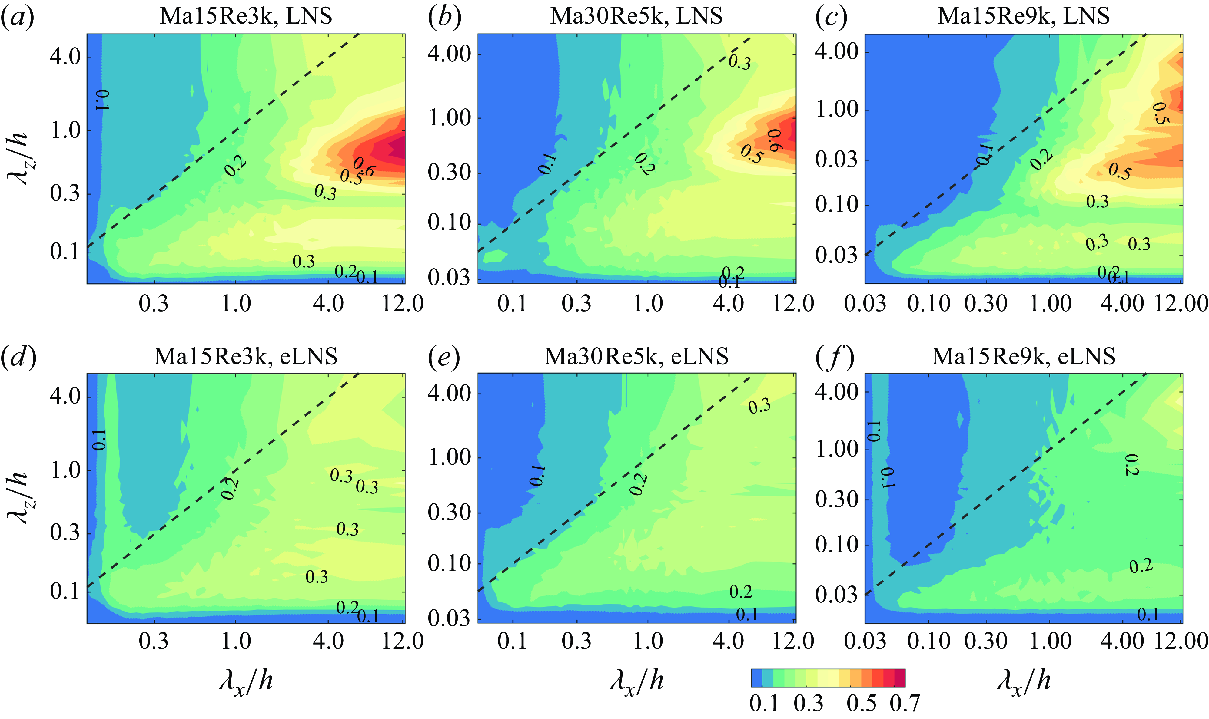
Figure 12. Energy ratio occupied by the leading POD mode (
 $r_{\sigma ,1}=\sigma _1/\sum _j\sigma _j$
) for the forcing in the (a,b,c) LNS and (d,e,f) eLNS models at different
$r_{\sigma ,1}=\sigma _1/\sum _j\sigma _j$
) for the forcing in the (a,b,c) LNS and (d,e,f) eLNS models at different
 $\lambda _x$
,
$\lambda _x$
,
 $\lambda _z$
for cases (a,d) Ma15Re3k, (b,e) Ma30Re5k and (c,f) Ma15Re9k. The black dashed line denotes
$\lambda _z$
for cases (a,d) Ma15Re3k, (b,e) Ma30Re5k and (c,f) Ma15Re9k. The black dashed line denotes
 $\lambda _x=\lambda _z$
.
$\lambda _x=\lambda _z$
.
For a more quantitative comparison of
 $r_{\sigma ,1}$
between different cases, its variation with
$r_{\sigma ,1}$
between different cases, its variation with
 $\lambda _z/h$
is plotted in figure 13 for all three compressible cases, at the largest streamwise scale
$\lambda _z/h$
is plotted in figure 13 for all three compressible cases, at the largest streamwise scale
 $\lambda _x=4\pi h$
. The two incompressible cases are also included for reference. Cases Ma00Re3k, Ma15Re3k and Ma30Re5k have comparable
$\lambda _x=4\pi h$
. The two incompressible cases are also included for reference. Cases Ma00Re3k, Ma15Re3k and Ma30Re5k have comparable
 $\textit{Re}_\tau ^*=141\!\sim \!186$
, and their
$\textit{Re}_\tau ^*=141\!\sim \!186$
, and their
 $r_{\sigma ,1}$
values are also close to each other, except at the very small scale. For the two higher
$r_{\sigma ,1}$
values are also close to each other, except at the very small scale. For the two higher
 $\textit{Re}_\tau ^*$
cases Ma15Re9k and Ma00Re10k, their
$\textit{Re}_\tau ^*$
cases Ma15Re9k and Ma00Re10k, their
 $r_{\sigma ,1}$
also have analogous distributions. Therefore, it is concluded that the low-rank feature of the LNS forcing is not sensitive to
$r_{\sigma ,1}$
also have analogous distributions. Therefore, it is concluded that the low-rank feature of the LNS forcing is not sensitive to
 ${\textit {Ma}}_b$
, although a higher
${\textit {Ma}}_b$
, although a higher
 ${\textit {Ma}}_b$
can slightly decrease
${\textit {Ma}}_b$
can slightly decrease
 $r_{\sigma ,1}$
due to the increasing acoustic components (see § 5). Meanwhile, the low-rank feature is weakened by a rising
$r_{\sigma ,1}$
due to the increasing acoustic components (see § 5). Meanwhile, the low-rank feature is weakened by a rising
 $\textit{Re}_\tau$
, suggesting reduced spatial-temporal coherence as turbulence intensifies.
$\textit{Re}_\tau$
, suggesting reduced spatial-temporal coherence as turbulence intensifies.
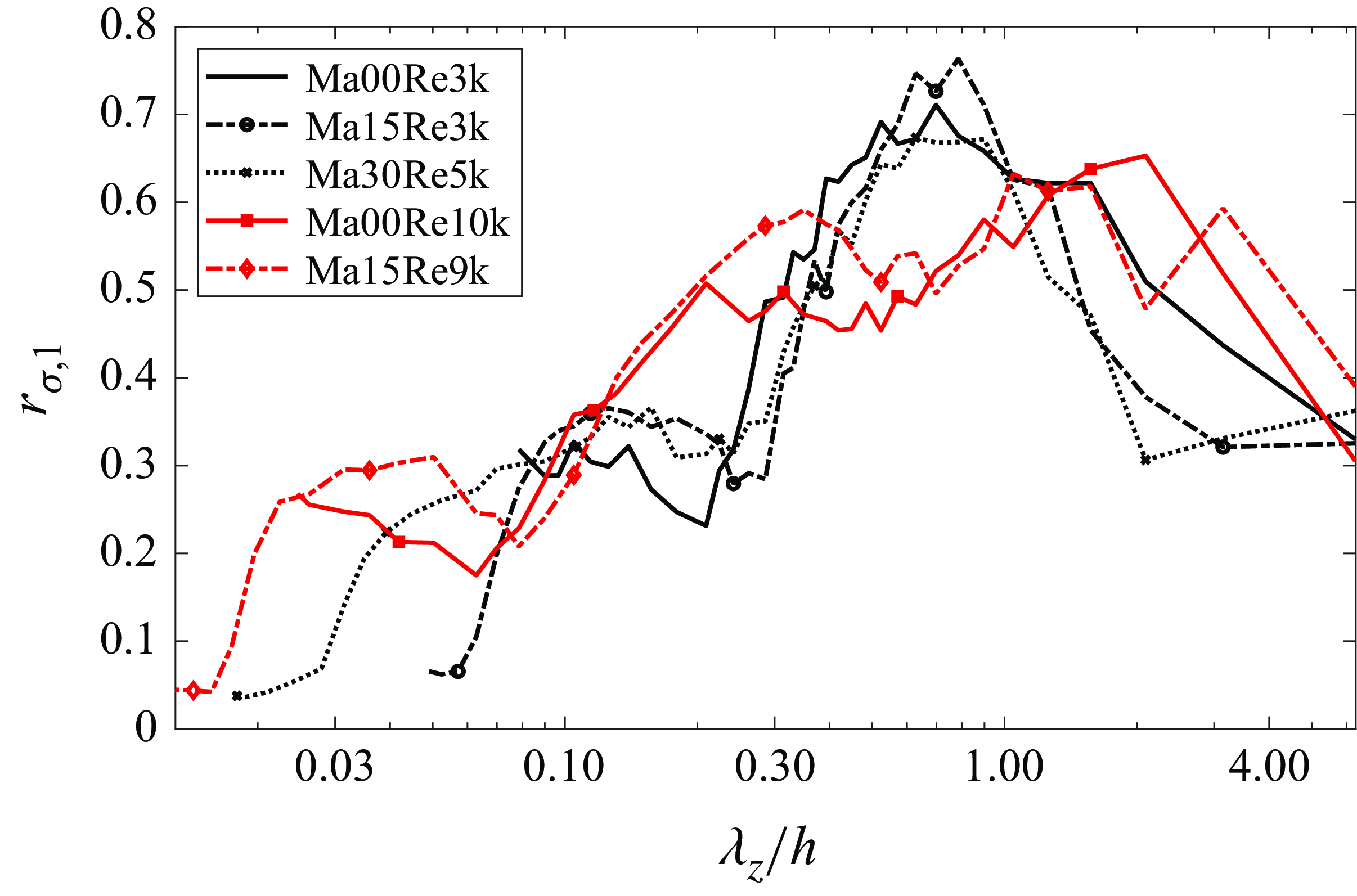
Figure 13. Energy ratio of the leading POD mode (
 $r_{\sigma ,1}$
) for the LNS forcing with different
$r_{\sigma ,1}$
) for the LNS forcing with different
 $\lambda _z$
for different cases (at largest
$\lambda _z$
for different cases (at largest
 $\lambda _x=4\pi h$
). Cases Ma00Re3k, Ma15Re3k and Ma30Re5k have comparable
$\lambda _x=4\pi h$
). Cases Ma00Re3k, Ma15Re3k and Ma30Re5k have comparable
 $\textit{Re}_\tau ^*=141\!\sim \!186$
; cases Ma15Re9k and Ma00Re10k have higher
$\textit{Re}_\tau ^*=141\!\sim \!186$
; cases Ma15Re9k and Ma00Re10k have higher
 $\textit{Re}_\tau ^*=393$
and 547 (see table 2).
$\textit{Re}_\tau ^*=393$
and 547 (see table 2).
Regarding the eLNS results, figure 12 shows that the eLNS model largely disrupts the low-rank feature of the LNS forcing for scales
 $\lambda _x\gt \lambda _z$
, by including the eddy-viscosity-enhanced terms. The large-scale fluctuations of high linear coherence are particularly affected, with
$\lambda _x\gt \lambda _z$
, by including the eddy-viscosity-enhanced terms. The large-scale fluctuations of high linear coherence are particularly affected, with
 $r_{\sigma ,1}$
down to
$r_{\sigma ,1}$
down to
 $\lesssim {30}\,\%$
, so these scales are the region where the prediction of the linear coherence is mostly improved by the eLNS model over LNS. For other scales (
$\lesssim {30}\,\%$
, so these scales are the region where the prediction of the linear coherence is mostly improved by the eLNS model over LNS. For other scales (
 $\lambda _x\lt \lambda _z$
, or small
$\lambda _x\lt \lambda _z$
, or small
 $\lambda _z$
), the improvement by eLNS is not obvious. Further improvements are anticipated by optimising the
$\lambda _z$
), the improvement by eLNS is not obvious. Further improvements are anticipated by optimising the
 $\mu _t$
profile for different scales, as realised by Symon et al. (Reference Symon, Madhusudanan, Illingworth and Marusic2023) and Ying et al. (Reference Ying, Chen, Li and Fu2024a
) for incompressible flows, and by considering inter-variable correlations.
$\mu _t$
profile for different scales, as realised by Symon et al. (Reference Symon, Madhusudanan, Illingworth and Marusic2023) and Ying et al. (Reference Ying, Chen, Li and Fu2024a
) for incompressible flows, and by considering inter-variable correlations.
5. Role of acoustic modes
It is known that the fluctuations in compressible flows can be decomposed into the vortical, acoustic and entropy components (Kovasznay Reference Kovasznay1953). The latter two are absent in incompressible flows, and are primarily responsible for intrinsic compressibility effects. The acoustic modes were shown to result in distinct features of the linear models from the incompressible counterpart (Jeun, Nichols & Jovanović Reference Jeun, Nichols and Jovanović2016; Bae et al. Reference Bae, Dawson and McKeon2020; Madhusudanan et al. Reference Madhusudanan, Stroot and McKeon2025), such as centred fluctuations around the relative sonic line and notable Mach-wave radiation into the free
stream. Particularly, Chen et al. (Reference Chen, Cheng, Gan and Fu2023b
) found that overly
predicted acoustic modes can severely degrade the performance of stochastic linear models in estimating wall-normally coherent density and temperature fluctuations (i.e. the components of
 $\langle \hat {\boldsymbol q}^{{\kern0.3pt}{\prime \prime }}\hat {\boldsymbol q}^{{{\prime \prime }}{{H}}} \rangle$
). When using (2.15) as the forcing model, for example, they showed that the predicted acoustic and entropy modes can contribute up to 55 % of the response growth. Although, they pointed out that such a high energy portion contradicted the DNS data (their figures 5 and 14), the real energy portion was not revealed.
$\langle \hat {\boldsymbol q}^{{\kern0.3pt}{\prime \prime }}\hat {\boldsymbol q}^{{{\prime \prime }}{{H}}} \rangle$
). When using (2.15) as the forcing model, for example, they showed that the predicted acoustic and entropy modes can contribute up to 55 % of the response growth. Although, they pointed out that such a high energy portion contradicted the DNS data (their figures 5 and 14), the real energy portion was not revealed.
Here, we assess quantitatively the role of the acoustic components within the current linear-model framework using the DNS data. We first seek to extract the acoustic components out of
 $\langle \hat {\boldsymbol q}^{{\kern0.3pt}{\prime \prime }}\hat {\boldsymbol q}^{{{\prime \prime }}{{H}}} \rangle$
and the forcing matrix, and then discuss the key characteristics of these acoustic components.
$\langle \hat {\boldsymbol q}^{{\kern0.3pt}{\prime \prime }}\hat {\boldsymbol q}^{{{\prime \prime }}{{H}}} \rangle$
and the forcing matrix, and then discuss the key characteristics of these acoustic components.
5.1. Pressure decomposition for acoustic fluctuations
One viable path to extract the acoustic fluctuations is to first decompose the pressure fluctuation
 $p^\prime$
based on the pressure Poisson equation, and then formulate other acoustic variables based on the compressible part of
$p^\prime$
based on the pressure Poisson equation, and then formulate other acoustic variables based on the compressible part of
 $p^\prime$
. The first step is conducted in this subsection.
$p^\prime$
. The first step is conducted in this subsection.
Following Sarkar (Reference Sarkar1992) and Zhang et al. (Reference Zhang, Wan, Sun and Lu2024),
 $p^{\prime }$
is decomposed into the quasi-incompressible part
$p^{\prime }$
is decomposed into the quasi-incompressible part
 $p_{ic}^{\prime }$
and the compressible part
$p_{ic}^{\prime }$
and the compressible part
 $p_c^{\prime }$
. The governing equations for the two are obtained by classifying the right-hand-side terms of the pressure Poisson equation, as
$p_c^{\prime }$
. The governing equations for the two are obtained by classifying the right-hand-side terms of the pressure Poisson equation, as
 $${\frac {\partial ^2 p_{ic}^{\prime }}{\partial x_i \partial x_i} = - 2\frac {\partial \tilde {u}_i}{\partial x_j} \frac {\partial \rho u_j^{{\prime \prime }}}{\partial x_i} - \frac {\partial ^2}{\partial x_i \partial x_j} \left ( \rho u_i^{{\prime \prime }} u_j^{{\prime \prime }} - \bar {\rho }\widetilde {u_i^{{\prime \prime }} u_j^{{\prime \prime }}} \right ) + \frac {\partial ^2 \tau _{ij}^{\prime }}{\partial x_i \partial x_j},}$$
 $${\frac {\partial p_c^{\prime }}{\partial x_i \partial x_i} = \frac {\partial ^2 \rho ^{\prime }}{\partial t^2} - \frac {\partial ^2 (\rho ^{\prime } \tilde {u}_i \tilde {u}_j )}{\partial x_i \partial x_j} - \tilde {u}_i \frac {\partial ^2 (2\rho u_j^{{\prime \prime }})}{\partial x_i \partial x_j} - \frac {\partial }{\partial x_i} \left (2 \rho u_i^{{\prime \prime }} \frac {\partial \tilde {u}_j}{\partial x_j}\right ).}$$
The boundary conditions are
 $\partial p_{ic}^{\prime }/\partial y=\partial \tau _{i2}^{\prime }/\partial x_i$
and
$\partial p_{ic}^{\prime }/\partial y=\partial \tau _{i2}^{\prime }/\partial x_i$
and
 $\partial p_c^{\prime }/\partial y=0$
at both wall sides (Yu, Xu & Pirozzoli Reference Yu, Xu and Pirozzoli2020). For incompressible flows,
$\partial p_c^{\prime }/\partial y=0$
at both wall sides (Yu, Xu & Pirozzoli Reference Yu, Xu and Pirozzoli2020). For incompressible flows,
 $p_c^{\prime }$
naturally reduces to zero since
$p_c^{\prime }$
naturally reduces to zero since
 $\rho ^{\prime }=\partial \tilde {u}_j/\partial x_j=\partial {u}_j^{{\prime \prime }}/\partial x_j=0$
. The part
$\rho ^{\prime }=\partial \tilde {u}_j/\partial x_j=\partial {u}_j^{{\prime \prime }}/\partial x_j=0$
. The part
 $p_{ic}^{\prime }$
can be further decomposed (into a rapid term, etc.), but here, we simply treat it as a whole, as we focus on the compressibility effects. In this sense,
$p_{ic}^{\prime }$
can be further decomposed (into a rapid term, etc.), but here, we simply treat it as a whole, as we focus on the compressibility effects. In this sense,
 $p_{ic}^{\prime }$
reflects the collective contribution of vortical modes, while
$p_{ic}^{\prime }$
reflects the collective contribution of vortical modes, while
 $p_c^{\prime }$
is mainly contributed by acoustic modes. Equation (5.1) is solved using the Fourier–Galerkin scheme. Since the temporal derivative in (5.1b
) is not available in our time-not-resolved data, we obtain
$p_c^{\prime }$
is mainly contributed by acoustic modes. Equation (5.1) is solved using the Fourier–Galerkin scheme. Since the temporal derivative in (5.1b
) is not available in our time-not-resolved data, we obtain
 $p_c^{\prime }$
simply from
$p_c^{\prime }$
simply from
 $p_c^{\prime }=p^{\prime }-p_{ic}^{\prime }$
after solving
$p_c^{\prime }=p^{\prime }-p_{ic}^{\prime }$
after solving
 $p_{ic}^{\prime }$
from (5.1a
). The accuracy of
$p_{ic}^{\prime }$
from (5.1a
). The accuracy of
 $p_c^{\prime }$
is reliable because the realistic
$p_c^{\prime }$
is reliable because the realistic
 $p^{\prime }$
and that solved from the Poisson equation were shown to differ by less than 1 % for similar channel cases (Yu et al. Reference Yu, Xu and Pirozzoli2020).
$p^{\prime }$
and that solved from the Poisson equation were shown to differ by less than 1 % for similar channel cases (Yu et al. Reference Yu, Xu and Pirozzoli2020).

Figure 14. (a) Variance and correlation of pressure fluctuation components for cases Ma15Re3k and Ma30Re5k. (b
 $-$
e) Pre-multiplied 2-D spectra for the (b,d) incompressible and (c,e) compressible parts of the wall pressure fluctuations for cases (b,c) Ma15Re3k and (d,e) Ma30Re5k. The black dashed line in the right four panels denotes
$-$
e) Pre-multiplied 2-D spectra for the (b,d) incompressible and (c,e) compressible parts of the wall pressure fluctuations for cases (b,c) Ma15Re3k and (d,e) Ma30Re5k. The black dashed line in the right four panels denotes
 $\lambda _x=\lambda _z$
.
$\lambda _x=\lambda _z$
.
The variances of the pressure and its components for cases Ma15Re3k and Ma30Re5k are plotted in figure 14(a), where the normalisation is
 $p^{{\prime }+}=p^{\prime }/\tau _w$
. After the decomposition, the
$p^{{\prime }+}=p^{\prime }/\tau _w$
. After the decomposition, the
 $p_{ic,\textit {rms}}^{{\prime }+}$
in the two cases are close to each other under the same
$p_{ic,\textit {rms}}^{{\prime }+}$
in the two cases are close to each other under the same
 $\textit{Re}_\tau ^*$
, suggesting robust contributions from the quasi-incompressible part. If
$\textit{Re}_\tau ^*$
, suggesting robust contributions from the quasi-incompressible part. If
 $p_{ic}^{{\prime }+}$
is regarded as the result at
$p_{ic}^{{\prime }+}$
is regarded as the result at
 ${\textit {Ma}}_b=0$
, then the wall pressure variance roughly follows a linear relation
${\textit {Ma}}_b=0$
, then the wall pressure variance roughly follows a linear relation
 \begin{equation} \overline {p_w^{{\prime }+2}}({\textit {Ma}}_b) \approx \overline {p_w^{{\prime }+2}}(0) + 0.216{\textit {Ma}}_b^2, \quad \text{for}\; \textit{Re}_\tau ^*\approx 140. \end{equation}
This scaling is consistent with Yu et al. (Reference Yu, Xu and Pirozzoli2020) although the slope differs due to a different
 $\textit{Re}$
. With
$\textit{Re}$
. With
 ${\textit {Ma}}_b$
increased,
${\textit {Ma}}_b$
increased,
 $p_{c,\textit {rms}}^{{\prime }+}$
quickly rises and surpasses
$p_{c,\textit {rms}}^{{\prime }+}$
quickly rises and surpasses
 $p^{{\prime }+}_{ic,\textit {rms}}$
at
$p^{{\prime }+}_{ic,\textit {rms}}$
at
 ${\textit {Ma}}_b=3$
at the wall. Moreover,
${\textit {Ma}}_b=3$
at the wall. Moreover,
 $p_{c,\textit {rms}}^{{\prime }+}$
is mostly amplified near the wall, suggesting locally intensified fluctuations of mass flux. The correlation
$p_{c,\textit {rms}}^{{\prime }+}$
is mostly amplified near the wall, suggesting locally intensified fluctuations of mass flux. The correlation
 $\overline {p_{ic}^{{\prime }+}p_c^{{\prime }+}}$
is also plotted, which remains small (
$\overline {p_{ic}^{{\prime }+}p_c^{{\prime }+}}$
is also plotted, which remains small (
 ${\lt } 0.2$
) throughout the field for both cases.
${\lt } 0.2$
) throughout the field for both cases.
Furthermore, the pre-multiplied 2-D spectra of
 $\hat {p}_{ic}^{\prime }$
and
$\hat {p}_{ic}^{\prime }$
and
 $\hat {p}_{c}^{\prime }$
at the wall are displayed in figure 14. The pressure spectra in compressible flows have been comprehensively studied before (Bernardini & Pirozzoli Reference Bernardini and Pirozzoli2011; Duan, Choudhari & Zhang Reference Duan, Choudhari and Zhang2016). Our intention here is to provide further support to the decomposition (5.1), by demonstrating the resemblance of the
$\hat {p}_{c}^{\prime }$
at the wall are displayed in figure 14. The pressure spectra in compressible flows have been comprehensively studied before (Bernardini & Pirozzoli Reference Bernardini and Pirozzoli2011; Duan, Choudhari & Zhang Reference Duan, Choudhari and Zhang2016). Our intention here is to provide further support to the decomposition (5.1), by demonstrating the resemblance of the
 $\hat {p}_{ic}^{\prime }$
spectra under different
$\hat {p}_{ic}^{\prime }$
spectra under different
 ${\textit {Ma}}_b$
and the clear scale separation between
${\textit {Ma}}_b$
and the clear scale separation between
 $\hat {p}_{ic}^{\prime }$
and
$\hat {p}_{ic}^{\prime }$
and
 $\hat {p}_{c}^{\prime }$
. The part
$\hat {p}_{c}^{\prime }$
. The part
 $\hat {p}_{c}^{\prime }$
resides at much smaller streamwise scales than
$\hat {p}_{c}^{\prime }$
resides at much smaller streamwise scales than
 $\hat {p}_{ic}^{\prime }$
, taking the form of travelling waves, so
$\hat {p}_{ic}^{\prime }$
, taking the form of travelling waves, so
 $\hat {p}_{c}^{\prime }$
turns out to be spanwise
elongated with the peak locating at
$\hat {p}_{c}^{\prime }$
turns out to be spanwise
elongated with the peak locating at
 $(\lambda _x,\lambda _z)/h\approx (0.5,1)$
for case Ma30Re5k.
$(\lambda _x,\lambda _z)/h\approx (0.5,1)$
for case Ma30Re5k.
5.2. Variance and structure of acoustic components
The
 $\hat {p}_c^{\prime }$
obtained in § 5.1 can be utilised to recover the other variables of acoustic modes. From 1-D eigenmode analysis, the
$\hat {p}_c^{\prime }$
obtained in § 5.1 can be utilised to recover the other variables of acoustic modes. From 1-D eigenmode analysis, the
 $\hat {\boldsymbol q}^{{\kern0.3pt}{\prime \prime }}$
of acoustic modes, denoted as
$\hat {\boldsymbol q}^{{\kern0.3pt}{\prime \prime }}$
of acoustic modes, denoted as
 $\hat {\boldsymbol q}_{\textit {ac}}^{{\prime \prime }}$
, is related to
$\hat {\boldsymbol q}_{\textit {ac}}^{{\prime \prime }}$
, is related to
 $\hat {p}_c^{\prime }$
as
$\hat {p}_c^{\prime }$
as
 \begin{equation} \hat {\boldsymbol q}_{\textit {ac}}^{{\prime \prime }} = \big[\rho _{\textit {ac}}^{\prime },\,u_{\textit {ac}}^{{\prime \prime }},\,v_{\textit {ac}}^{{\prime \prime }},\,w_{\textit {ac}}^{{\prime \prime }},\,T_{\textit {ac}}^{{\prime \prime }}\big]^{T} = \frac {\boldsymbol{C}_{\textit {vis}}}{\gamma \bar {p}} \left [ \bar {\rho },\, \frac {k_xa}{k}, -\frac {{\mathrm{i}} a}{k}\frac {{{d}}}{{\mathrm{d}} y},\, \frac {k_za}{k},\, (\gamma -1)\widetilde {T} \right ]^{T} \hat {p}_c^{\prime }, \end{equation}
where
 $k^2=k_x^2+k_z^2$
. Derivation of (5.3) is detailed in
Appendix C. Consequently, the acoustic part
$k^2=k_x^2+k_z^2$
. Derivation of (5.3) is detailed in
Appendix C. Consequently, the acoustic part
 $\langle \hat {\boldsymbol q}_{\textit {ac}}^{{\prime \prime }} \hat {\boldsymbol q}_{\textit {ac}}^{{{\prime \prime }}{{H}}} \rangle \equiv \langle \hat {\boldsymbol q}^{{\kern0.3pt}{\prime \prime }} \hat {\boldsymbol q}^{{{\prime \prime }}{{H}}} \rangle _{\textit {ac}}$
can be extracted out of
$\langle \hat {\boldsymbol q}_{\textit {ac}}^{{\prime \prime }} \hat {\boldsymbol q}_{\textit {ac}}^{{{\prime \prime }}{{H}}} \rangle \equiv \langle \hat {\boldsymbol q}^{{\kern0.3pt}{\prime \prime }} \hat {\boldsymbol q}^{{{\prime \prime }}{{H}}} \rangle _{\textit {ac}}$
can be extracted out of
 $\langle \hat {\boldsymbol q}^{{\kern0.3pt}{\prime \prime }} \hat {\boldsymbol q}^{{{\prime \prime }}{{H}}} \rangle$
, based on
$\langle \hat {\boldsymbol q}^{{\kern0.3pt}{\prime \prime }} \hat {\boldsymbol q}^{{{\prime \prime }}{{H}}} \rangle$
, based on
 $\langle \hat {p}_c^{\prime }\hat {p}_c^{{\prime }{{H}}} \rangle$
and (5.3). The residual
$\langle \hat {p}_c^{\prime }\hat {p}_c^{{\prime }{{H}}} \rangle$
and (5.3). The residual
 $\langle \hat {\boldsymbol q}^{{\kern0.3pt}{\prime \prime }} \hat {\boldsymbol q}^{{{\prime \prime }}{{H}}} \rangle _{\textit {nac}}=\langle \hat {\boldsymbol q}^{{\kern0.3pt}{\prime \prime }} \hat {\boldsymbol q}^{{{\prime \prime }}{{H}}} \rangle -\langle \hat {\boldsymbol q}^{{\kern0.3pt}{\prime \prime }} \hat {\boldsymbol q}^{{{\prime \prime }}{{H}}} \rangle _{\textit {ac}}$
is regarded as the non-acoustic part, which mostly comes from vortical modes although it also includes weak vortical–acoustic coupling. In the following, the relative contributions of
$\langle \hat {\boldsymbol q}^{{\kern0.3pt}{\prime \prime }} \hat {\boldsymbol q}^{{{\prime \prime }}{{H}}} \rangle _{\textit {nac}}=\langle \hat {\boldsymbol q}^{{\kern0.3pt}{\prime \prime }} \hat {\boldsymbol q}^{{{\prime \prime }}{{H}}} \rangle -\langle \hat {\boldsymbol q}^{{\kern0.3pt}{\prime \prime }} \hat {\boldsymbol q}^{{{\prime \prime }}{{H}}} \rangle _{\textit {ac}}$
is regarded as the non-acoustic part, which mostly comes from vortical modes although it also includes weak vortical–acoustic coupling. In the following, the relative contributions of
 $\langle \hat {\boldsymbol q}^{{\kern0.3pt}{\prime \prime }} \hat {\boldsymbol q}^{{{\prime \prime }}{{H}}} \rangle _{\textit {ac}}$
and
$\langle \hat {\boldsymbol q}^{{\kern0.3pt}{\prime \prime }} \hat {\boldsymbol q}^{{{\prime \prime }}{{H}}} \rangle _{\textit {ac}}$
and
 $\langle \hat {\boldsymbol q}^{{\kern0.3pt}{\prime \prime }} \hat {\boldsymbol q}^{{{\prime \prime }}{{H}}} \rangle _{\textit {nac}}$
are assessed, and the two are further utilised to decompose the forcing, which will uncover the quantitative contribution of the acoustic components in the stochastic linear model.
$\langle \hat {\boldsymbol q}^{{\kern0.3pt}{\prime \prime }} \hat {\boldsymbol q}^{{{\prime \prime }}{{H}}} \rangle _{\textit {nac}}$
are assessed, and the two are further utilised to decompose the forcing, which will uncover the quantitative contribution of the acoustic components in the stochastic linear model.
Equation (5.3) explicitly indicates the scale dependence of
 $\hat {\boldsymbol q}_{\textit {ac}}^{{\prime \prime }}$
. The ratios
$\hat {\boldsymbol q}_{\textit {ac}}^{{\prime \prime }}$
. The ratios
 $\hat {\rho }_{\textit {ac}}^{\prime }/\hat {p}_c^{\prime }$
and
$\hat {\rho }_{\textit {ac}}^{\prime }/\hat {p}_c^{\prime }$
and
 $\hat {T}_{\textit {ac}}^{{\prime \prime }}/\hat {p}_c^{\prime }$
turn out to be nearly independent of
$\hat {T}_{\textit {ac}}^{{\prime \prime }}/\hat {p}_c^{\prime }$
turn out to be nearly independent of
 $k_x$
and
$k_x$
and
 $k_z$
, so the spectral distributions of
$k_z$
, so the spectral distributions of
 $\hat {\rho }_{\textit {ac}}^{\prime }$
and
$\hat {\rho }_{\textit {ac}}^{\prime }$
and
 $\hat {T}_{\textit {ac}}^{{\prime \prime }}$
are primarily determined by
$\hat {T}_{\textit {ac}}^{{\prime \prime }}$
are primarily determined by
 $\hat {p}_c^{\prime }$
and the mean flow. Regarding the velocity components, the relation
$\hat {p}_c^{\prime }$
and the mean flow. Regarding the velocity components, the relation
 $\hat {u}_{\textit {ac}}^{{\prime \prime }}\ll \hat {w}_{\textit {ac}}^{{\prime \prime }}$
holds if
$\hat {u}_{\textit {ac}}^{{\prime \prime }}\ll \hat {w}_{\textit {ac}}^{{\prime \prime }}$
holds if
 $k_x\ll k_z$
, so the acoustic motion for streamwise-elongated structures is mainly active in the
$k_x\ll k_z$
, so the acoustic motion for streamwise-elongated structures is mainly active in the
 $y$
–
$y$
–
 $z$
plane with velocities
$z$
plane with velocities
 $\hat {v}_{\textit {ac}}^{{\prime \prime }}$
and
$\hat {v}_{\textit {ac}}^{{\prime \prime }}$
and
 $\hat {w}_{\textit {ac}}^{{\prime \prime }}$
. Conversely, the acoustic motion is constrained in the
$\hat {w}_{\textit {ac}}^{{\prime \prime }}$
. Conversely, the acoustic motion is constrained in the
 $x$
–
$x$
–
 $y$
plane for spanwise-elongated structures when
$y$
plane for spanwise-elongated structures when
 $k_x\gg k_z$
.
$k_x\gg k_z$
.
The
 $\hat {p}_c^{\prime }$
value in the two
$\hat {p}_c^{\prime }$
value in the two
 ${\textit {Ma}}_b=1.5$
cases is relatively low, so we focus on case Ma30Re5k to see the potential effects of acoustic modes. Before inspecting
${\textit {Ma}}_b=1.5$
cases is relatively low, so we focus on case Ma30Re5k to see the potential effects of acoustic modes. Before inspecting
 $\hat {\boldsymbol q}_{\textit {ac}}^{{\prime \prime }}$
, we first examine the spectral distribution of the relative strength of
$\hat {\boldsymbol q}_{\textit {ac}}^{{\prime \prime }}$
, we first examine the spectral distribution of the relative strength of
 $\hat {p}_c^{\prime }$
and
$\hat {p}_c^{\prime }$
and
 $\hat {p}_{ic}^{\prime }$
. To reflect their amplitudes at different scales, the energy norm for pressure is defined as (Chu Reference Chu1965)
$\hat {p}_{ic}^{\prime }$
. To reflect their amplitudes at different scales, the energy norm for pressure is defined as (Chu Reference Chu1965)
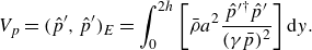 \begin{equation} V_p = ( \hat {p}^{\prime }, \hat {p}^{\prime } )_E = \int _{0}^{2h} { \left [ \bar {\rho } a^2 \frac {\hat {p}^{{\prime }\dagger }\hat {p}^{{\prime }}}{(\gamma \bar {p})^2} \right ] {\mathrm{d}} y}. \end{equation}
Figure 15 provides the distributions of three norm ratios of the pressure components among all scales: the compressible part
 $r_{p_c}=(\hat {p}_c^{\prime },\hat {p}_c^{\prime })_E/V_p$
, the incompressible part
$r_{p_c}=(\hat {p}_c^{\prime },\hat {p}_c^{\prime })_E/V_p$
, the incompressible part
 $r_{p_i}=(\hat {p}_{ic}^{\prime },\hat {p}_{ic}^{\prime })_E/V_p$
and their coupling
$r_{p_i}=(\hat {p}_{ic}^{\prime },\hat {p}_{ic}^{\prime })_E/V_p$
and their coupling
 $r_{p_cp_i}=(\hat {p}_{c}^{\prime },\hat {p}_{ic}^{\prime })_E/V_p$
. Based on these ratios, three distinct regions in terms of the horizontal scales
$r_{p_cp_i}=(\hat {p}_{c}^{\prime },\hat {p}_{ic}^{\prime })_E/V_p$
. Based on these ratios, three distinct regions in terms of the horizontal scales
 $(\lambda _x,\lambda _z)$
can be divided, as denoted by the dashed lines (see figure 15
c). The first region (I) is of either small
$(\lambda _x,\lambda _z)$
can be divided, as denoted by the dashed lines (see figure 15
c). The first region (I) is of either small
 $\lambda _x^+$
or
$\lambda _x^+$
or
 $\lambda _z^+$
(
$\lambda _z^+$
(
 $\lesssim 30$
), where
$\lesssim 30$
), where
 $r_{p_c}$
exceeds 40 % and
$r_{p_c}$
exceeds 40 % and
 $r_{p_i}$
falls below 50 % and can down to 10 %. These fluctuations reside near the wall where
$r_{p_i}$
falls below 50 % and can down to 10 %. These fluctuations reside near the wall where
 $p_{c}^{{\prime }}$
is the strongest, so they are most affected by acoustic modes, resulting in deviations from their incompressible counterpart. The second region (II) comprises the streamwise-elongated fluctuations of high linear coherence (
$p_{c}^{{\prime }}$
is the strongest, so they are most affected by acoustic modes, resulting in deviations from their incompressible counterpart. The second region (II) comprises the streamwise-elongated fluctuations of high linear coherence (
 $\lambda _z^+\gt 30$
). They are nearly unaffected by
$\lambda _z^+\gt 30$
). They are nearly unaffected by
 $p_c^{\prime }$
with
$p_c^{\prime }$
with
 $r_{p_i}$
over 90 %, so they are dominated by vortical modes. The slightly higher
$r_{p_i}$
over 90 %, so they are dominated by vortical modes. The slightly higher
 $r_{p_c}$
for the largest scale in the domain
$r_{p_c}$
for the largest scale in the domain
 $(\lambda _x,\lambda _z)/h=(4\pi ,2\pi )$
may be attributed to the artificial scale truncation by the domain size. In comparison, the spanwise-elongated ones in region III feature higher
$(\lambda _x,\lambda _z)/h=(4\pi ,2\pi )$
may be attributed to the artificial scale truncation by the domain size. In comparison, the spanwise-elongated ones in region III feature higher
 $r_{p_c}\gtrsim {20}\,\%$
and stronger
$r_{p_c}\gtrsim {20}\,\%$
and stronger
 $\hat {p}_c^{\prime }$
–
$\hat {p}_c^{\prime }$
–
 $\hat {p}_i^{\prime }$
coupling with
$\hat {p}_i^{\prime }$
coupling with
 $|r_{p_cp_i}|$
over 10 %, which is in line with the active zone of
$|r_{p_cp_i}|$
over 10 %, which is in line with the active zone of
 $p_{c,w}^{\prime }$
in figure 14(e).
$p_{c,w}^{\prime }$
in figure 14(e).

Figure 15. Energy norm ratios of (a) the compressible part
 $\langle \hat {p}_c^{\prime }\hat {p}_c^{{\prime }{{H}}} \rangle$
, (b) the incompressible part
$\langle \hat {p}_c^{\prime }\hat {p}_c^{{\prime }{{H}}} \rangle$
, (b) the incompressible part
 $\langle \hat {p}_{ic}^{\prime }\hat {p}_{ic}^{{\prime }{{H}}} \rangle$
and (c) their coupling
$\langle \hat {p}_{ic}^{\prime }\hat {p}_{ic}^{{\prime }{{H}}} \rangle$
and (c) their coupling
 $\langle \hat {p}_c^{\prime }\hat {p}_{ic}^{{\prime }{{H}}} \rangle$
relative to
$\langle \hat {p}_c^{\prime }\hat {p}_{ic}^{{\prime }{{H}}} \rangle$
relative to
 $\langle \hat {p}^{\prime }\hat {p}^{{\prime }{{H}}} \rangle$
for case Ma30Re5k. Three featured regions (I, II, III) are divided by the three black dashed lines
$\langle \hat {p}^{\prime }\hat {p}^{{\prime }{{H}}} \rangle$
for case Ma30Re5k. Three featured regions (I, II, III) are divided by the three black dashed lines
 $\lambda _x=\lambda _z$
,
$\lambda _x=\lambda _z$
,
 $\lambda _x^+=30$
and
$\lambda _x^+=30$
and
 $\lambda _z^+=30$
. Extra contours outside the shaded levels are shown in grey dashed lines with labelled levels.
$\lambda _z^+=30$
. Extra contours outside the shaded levels are shown in grey dashed lines with labelled levels.

Figure 16. (a) Pre-multiplied 2-D spectrum of the acoustic energy
 $V_{q_{\textit {ac}}}$
(normalised by
$V_{q_{\textit {ac}}}$
(normalised by
 $\rho _bU_b^2/h$
) and the energy-norm ratios of (b)
$\rho _bU_b^2/h$
) and the energy-norm ratios of (b)
 $\langle \,\hat {\!\boldsymbol q}^{{\prime \prime }}\,\hat {\!\boldsymbol q}^{{{\prime \prime }}{{H}}} \rangle _{\textit {ac}}$
and (c)
$\langle \,\hat {\!\boldsymbol q}^{{\prime \prime }}\,\hat {\!\boldsymbol q}^{{{\prime \prime }}{{H}}} \rangle _{\textit {ac}}$
and (c)
 $\langle \hat {\rho }^{\prime } \hat {\rho }^{{\prime }{{H}}} \rangle _{\textit {ac}}$
relative to
$\langle \hat {\rho }^{\prime } \hat {\rho }^{{\prime }{{H}}} \rangle _{\textit {ac}}$
relative to
 $\langle \,\hat {\!\boldsymbol q}^{{\prime \prime }}\,\hat {\!\boldsymbol q}^{{{\prime \prime }}{{H}}} \rangle$
and
$\langle \,\hat {\!\boldsymbol q}^{{\prime \prime }}\,\hat {\!\boldsymbol q}^{{{\prime \prime }}{{H}}} \rangle$
and
 $\langle \hat {\rho }^{\prime } \hat {\rho }^{{\prime }{{H}}} \rangle$
, respectively, for case Ma30Re5k. Three regions (I, II, III) are divided as in figure 15. The dotted lines in panel (a) are the contours (0.2, 0.4, 0.6, 0.8) of the normalised pre-multiplied spectrum of the total energy
$\langle \hat {\rho }^{\prime } \hat {\rho }^{{\prime }{{H}}} \rangle$
, respectively, for case Ma30Re5k. Three regions (I, II, III) are divided as in figure 15. The dotted lines in panel (a) are the contours (0.2, 0.4, 0.6, 0.8) of the normalised pre-multiplied spectrum of the total energy
 $V_q$
.
$V_q$
.
Next, the variance of
 $\hat {\boldsymbol q}_{\textit {ac}}^{{\prime \prime }}$
, i.e.
$\hat {\boldsymbol q}_{\textit {ac}}^{{\prime \prime }}$
, i.e.
 $V_{q_{\textit {ac}}}=\|\hat {\boldsymbol q}_{\textit {ac}}^{{\prime \prime }}\|^2$
, is computed, which reflects how much energy is contributed by acoustic modes to the total fluctuation energy in the linear models. The pre-multiplied 2-D spectrum of
$V_{q_{\textit {ac}}}=\|\hat {\boldsymbol q}_{\textit {ac}}^{{\prime \prime }}\|^2$
, is computed, which reflects how much energy is contributed by acoustic modes to the total fluctuation energy in the linear models. The pre-multiplied 2-D spectrum of
 $V_{q_{\textit {ac}}}$
is first plotted in figure 16(a), along with the
$V_{q_{\textit {ac}}}$
is first plotted in figure 16(a), along with the
 $V_q$
spectrum to show the region of energetic total fluctuations. The energy
$V_q$
spectrum to show the region of energetic total fluctuations. The energy
 $V_{q_{\textit {ac}}}$
is more pronounced at scales
$V_{q_{\textit {ac}}}$
is more pronounced at scales
 $\lambda _x\lt \lambda _z$
, consistent with figure 14(e). The ratio
$\lambda _x\lt \lambda _z$
, consistent with figure 14(e). The ratio
 $r_{q_{\textit {ac}}}=V_{q_{\textit {ac}}}/V_{q}$
for all scales is displayed in figure 16(b), whose pattern is qualitatively the same as in figure 15(a). The three distinct regions (I, II, III) analogous to figure 15 can be identified. The near-wall fluctuations of either small
$r_{q_{\textit {ac}}}=V_{q_{\textit {ac}}}/V_{q}$
for all scales is displayed in figure 16(b), whose pattern is qualitatively the same as in figure 15(a). The three distinct regions (I, II, III) analogous to figure 15 can be identified. The near-wall fluctuations of either small
 $\lambda _x^+$
or
$\lambda _x^+$
or
 $\lambda _z^+$
(
$\lambda _z^+$
(
 ${\lt } 30$
) are most susceptible to acoustic modes, with
${\lt } 30$
) are most susceptible to acoustic modes, with
 $r_{q_{\textit {ac}}}\gt {10}\,\%$
. This is consistent with Chen et al. (Reference Chen, Cheng, Fu and Gan2023a
) that the near-wall inner peak of the energy amplification curves, representing the optimal near-wall streak in the buffer layer, becomes non-existent with the rise of
$r_{q_{\textit {ac}}}\gt {10}\,\%$
. This is consistent with Chen et al. (Reference Chen, Cheng, Fu and Gan2023a
) that the near-wall inner peak of the energy amplification curves, representing the optimal near-wall streak in the buffer layer, becomes non-existent with the rise of
 ${\textit {Ma}}_b$
. In other words, the travelling-wave-like acoustic components disrupt the near-wall scaling of streamwise-elongated streaks and tend to dominate the near-wall turbulent motions.
${\textit {Ma}}_b$
. In other words, the travelling-wave-like acoustic components disrupt the near-wall scaling of streamwise-elongated streaks and tend to dominate the near-wall turbulent motions.
When
 $\lambda _x^+,\lambda _z^+\gt 30$
,
$\lambda _x^+,\lambda _z^+\gt 30$
,
 $r_{q_{\textit {ac}}}$
is generally less than 2 % for this
$r_{q_{\textit {ac}}}$
is generally less than 2 % for this
 ${\textit {Ma}}_b=3$
case, indicative of minor contributions from acoustic modes and dominance of vortical modes. This fact justifies the post-processing procedure of the cospectrum decomposition designed by Chen et al. (Reference Chen, Cheng, Gan and Fu2023b
), where the acoustic components are artificially removed from
${\textit {Ma}}_b=3$
case, indicative of minor contributions from acoustic modes and dominance of vortical modes. This fact justifies the post-processing procedure of the cospectrum decomposition designed by Chen et al. (Reference Chen, Cheng, Gan and Fu2023b
), where the acoustic components are artificially removed from
 $\langle \hat {\boldsymbol q}^{{\kern0.3pt}{\prime \prime }}\hat {\boldsymbol q}^{{{\prime \prime }}{{H}}} \rangle$
to improve the prediction of the linear coherence spectra of velocity and temperature in the eLNS model. The overly amplified acoustic components before the processing (
$\langle \hat {\boldsymbol q}^{{\kern0.3pt}{\prime \prime }}\hat {\boldsymbol q}^{{{\prime \prime }}{{H}}} \rangle$
to improve the prediction of the linear coherence spectra of velocity and temperature in the eLNS model. The overly amplified acoustic components before the processing (
 $r_{q_{\textit {ac}}}$
can reach 20%–55 % in their eLNS model under (2.15)) is due to misordered energies of the POD modes subject to an inaccurate forcing model.
$r_{q_{\textit {ac}}}$
can reach 20%–55 % in their eLNS model under (2.15)) is due to misordered energies of the POD modes subject to an inaccurate forcing model.
Regarding different components of
 $\hat {\boldsymbol q}_{\textit {ac}}^{{\prime \prime }}$
, the density fluctuation is most affected by the acoustic components. As shown in figure 16(c),
$\hat {\boldsymbol q}_{\textit {ac}}^{{\prime \prime }}$
, the density fluctuation is most affected by the acoustic components. As shown in figure 16(c),
 $r_{\rho _{\textit {ac}}}=\|\hat {\rho }_{\textit {ac}}^{\prime }\|^2/\|\hat {\rho }^{\prime }\|^2$
can surpass 10 % for spanwise-elongated fluctuations (region III). In comparison, the corresponding maximum ratios of the velocity components are all less than 3 %, so the velocities are dominated by vortical modes.
$r_{\rho _{\textit {ac}}}=\|\hat {\rho }_{\textit {ac}}^{\prime }\|^2/\|\hat {\rho }^{\prime }\|^2$
can surpass 10 % for spanwise-elongated fluctuations (region III). In comparison, the corresponding maximum ratios of the velocity components are all less than 3 %, so the velocities are dominated by vortical modes.

Figure 17. Profiles of the total density fluctuation variance and those contributed by the acoustic and non-acoustic parts for scales of (a)
 $(\lambda _x,\lambda _z)/h=(0.6,6.3)$
, (b)
$(\lambda _x,\lambda _z)/h=(0.6,6.3)$
, (b)
 $(\lambda _x,\lambda _z)/h=(12.6,6.3)$
and (c)
$(\lambda _x,\lambda _z)/h=(12.6,6.3)$
and (c)
 $(\lambda _x,\lambda _z)/h=(12.6,2.1)$
for case Ma30Re5k. Those predicted by the SRA relation (2.16) are also shown.
$(\lambda _x,\lambda _z)/h=(12.6,2.1)$
for case Ma30Re5k. Those predicted by the SRA relation (2.16) are also shown.
Considering the sensitivity of
 $r_{\rho _{\textit {ac}}}$
to acoustic modes, the wall-normal structure of
$r_{\rho _{\textit {ac}}}$
to acoustic modes, the wall-normal structure of
 $\hat {\rho }_{\textit {ac}}^{\prime }$
is presented in figure 17 using three selective scales. The first scale is
$\hat {\rho }_{\textit {ac}}^{\prime }$
is presented in figure 17 using three selective scales. The first scale is
 $(\lambda _x,\lambda _z)/h=(0.6,6.3)$
, corresponding to the peak of
$(\lambda _x,\lambda _z)/h=(0.6,6.3)$
, corresponding to the peak of
 $r_{q_{\textit {ac}}}$
(and
$r_{q_{\textit {ac}}}$
(and
 $r_{\rho _{\textit {ac}}}$
) in figure 16(b) in region III. The other two scales are both streamwise-elongated ones with
$r_{\rho _{\textit {ac}}}$
) in figure 16(b) in region III. The other two scales are both streamwise-elongated ones with
 $\lambda _x=12.6h$
and in different
$\lambda _x=12.6h$
and in different
 $\lambda _z$
. In figures 17(b) and 17(c),
$\lambda _z$
. In figures 17(b) and 17(c),
 $\hat {\rho }_{\textit {ac}}^{\prime }$
is much smaller than
$\hat {\rho }_{\textit {ac}}^{\prime }$
is much smaller than
 $\hat {\rho }_{\textit {nac}}^{\prime }$
, and the latter can be well approximated by the SRA relation (2.16). Therefore,
$\hat {\rho }_{\textit {nac}}^{\prime }$
, and the latter can be well approximated by the SRA relation (2.16). Therefore,
 $\hat {\rho }^{\prime }$
is transported like a passive scalar controlled by the mean-flow gradients for these streamwise-elongated motions (Coleman et al. Reference Coleman, Kim and Moser1995). Compared with the temperature part, the SRA for density has received less attention. Its effectiveness for these energetic motions also supports the usage of (2.15) for the density and temperature components. In figure 17(a) where
$\hat {\rho }^{\prime }$
is transported like a passive scalar controlled by the mean-flow gradients for these streamwise-elongated motions (Coleman et al. Reference Coleman, Kim and Moser1995). Compared with the temperature part, the SRA for density has received less attention. Its effectiveness for these energetic motions also supports the usage of (2.15) for the density and temperature components. In figure 17(a) where
 $r_{q_{\textit {ac}}}$
peaks, however,
$r_{q_{\textit {ac}}}$
peaks, however,
 $\hat {\rho }_{\textit {ac}}^{\prime }$
is more prominent and is higher than
$\hat {\rho }_{\textit {ac}}^{\prime }$
is more prominent and is higher than
 $\hat {\rho }_{\textit {nac}}^{\prime }$
near the wall. The
$\hat {\rho }_{\textit {nac}}^{\prime }$
near the wall. The
 $\hat {\rho }^{\prime }$
at the wall is almost solely contributed by
$\hat {\rho }^{\prime }$
at the wall is almost solely contributed by
 $\hat {\rho }_{\textit {ac}}^{\prime }$
, leaving the residual
$\hat {\rho }_{\textit {ac}}^{\prime }$
, leaving the residual
 $\hat {\rho }_{\textit {nac},w}^{\prime }$
nearly zero. This is reasonable because
$\hat {\rho }_{\textit {nac},w}^{\prime }$
nearly zero. This is reasonable because
 $\hat {\rho }_{\textit {nac}}^{\prime }$
is induced by vortical modes, then
$\hat {\rho }_{\textit {nac}}^{\prime }$
is induced by vortical modes, then
 $\hat {\rho }_{\textit {nac}}^{\prime }$
should tend to zero near the no-slip wall. The SRA relation (2.16) severely underestimates
$\hat {\rho }_{\textit {nac}}^{\prime }$
should tend to zero near the no-slip wall. The SRA relation (2.16) severely underestimates
 $\hat {\rho }_{\textit {nac}}^{\prime }$
at this scale because the localised spanwise motion (
$\hat {\rho }_{\textit {nac}}^{\prime }$
at this scale because the localised spanwise motion (
 $\hat {w}^{{\prime \prime }}$
) is active for these spanwise-elongated fluctuations.
$\hat {w}^{{\prime \prime }}$
) is active for these spanwise-elongated fluctuations.
The above decomposition of
 $\langle \hat {\boldsymbol q}^{{\kern0.3pt}{\prime \prime }} \hat {\boldsymbol q}^{{{\prime \prime }}{{H}}} \rangle$
into the acoustic and non-acoustic elements enables a decomposition of
$\langle \hat {\boldsymbol q}^{{\kern0.3pt}{\prime \prime }} \hat {\boldsymbol q}^{{{\prime \prime }}{{H}}} \rangle$
into the acoustic and non-acoustic elements enables a decomposition of
 $(\boldsymbol{{FF}}^{{H}})_{\textit{DNS}}$
and
$(\boldsymbol{{FF}}^{{H}})_{\textit{DNS}}$
and
 $(\boldsymbol{{EE}}^{{H}})_{\textit{DNS}}$
, which aids the respective modelling of the acoustic and non-acoustic parts of the forcing. From (2.19), the LNS forcing can be decomposed into
$(\boldsymbol{{EE}}^{{H}})_{\textit{DNS}}$
, which aids the respective modelling of the acoustic and non-acoustic parts of the forcing. From (2.19), the LNS forcing can be decomposed into
 $(\boldsymbol{{FF}}^{{H}})_{\textit{DNS}}=(\boldsymbol{{FF}}^{{H}})_{\textit{DNS},\textit {ac}}+(\boldsymbol{{FF}}^{{H}})_{\textit{DNS},\textit {nac}}$
, with the two parts satisfying
$(\boldsymbol{{FF}}^{{H}})_{\textit{DNS}}=(\boldsymbol{{FF}}^{{H}})_{\textit{DNS},\textit {ac}}+(\boldsymbol{{FF}}^{{H}})_{\textit{DNS},\textit {nac}}$
, with the two parts satisfying
 $${\big(\boldsymbol{{FF}}^{{H}}\big)_{\textit{DNS},\textit {ac}} = - \big ( \widehat {\mathcal{L}}_q \big\langle \hat {\boldsymbol q}^{{\kern0.3pt}{\prime \prime }} \hat {\boldsymbol q}^{{{\prime \prime }}{{H}}} \big\rangle _{\textit {ac}} + \big\langle \hat {\boldsymbol q}^{{\kern0.3pt}{\prime \prime }} \hat {\boldsymbol q}^{{{\prime \prime }}{{H}}} \big\rangle _{\textit {ac}} \widehat {\mathcal{L}}_q^{{H}} \big ),}$$
 $${\big(\boldsymbol{{FF}}^{{H}}\big)_{\textit{DNS},\textit {nac}} = - \big ( \widehat {\mathcal{L}}_q \big\langle \hat {\boldsymbol q}^{{\kern0.3pt}{\prime \prime }} \hat {\boldsymbol q}^{{{\prime \prime }}{{H}}} \big\rangle _{\textit {nac}} + \big\langle \hat {\boldsymbol q}^{{\kern0.3pt}{\prime \prime }} \hat {\boldsymbol q}^{{{\prime \prime }}{{H}}} \big\rangle _{\textit {nac}} \widehat {\mathcal{L}}_q^{{H}} \big ),}$$
respectively. The decomposition for the eLNS forcing is defined likewise. Different from vortical modes featuring strong non-normality, acoustic modes are nearly perpendicular to each other. Taking the leading acoustic modes (lowest frequency
 $|\omega |$
) as a representative,
$|\omega |$
) as a representative,
 $(\boldsymbol{{FF}}^{{H}})_{\textit{DNS},\textit {ac}}$
can be approximated as
$(\boldsymbol{{FF}}^{{H}})_{\textit{DNS},\textit {ac}}$
can be approximated as
 $-2\omega _{\textit {ac}} \langle \hat {\boldsymbol q}^{{\kern0.3pt}{\prime \prime }} \hat {\boldsymbol q}^{{{\prime \prime }}{{H}}} \rangle _{\textit {ac}}$
since
$-2\omega _{\textit {ac}} \langle \hat {\boldsymbol q}^{{\kern0.3pt}{\prime \prime }} \hat {\boldsymbol q}^{{{\prime \prime }}{{H}}} \rangle _{\textit {ac}}$
since
 $\widehat {\mathcal{L}}_q\,\check {\!\boldsymbol q}^{{\prime \prime }}=\omega _{\textit {ac}} \,\check {\!\boldsymbol q}^{{\prime \prime }}$
(details in Appendix C). Thereby, it can be conjectured that
$\widehat {\mathcal{L}}_q\,\check {\!\boldsymbol q}^{{\prime \prime }}=\omega _{\textit {ac}} \,\check {\!\boldsymbol q}^{{\prime \prime }}$
(details in Appendix C). Thereby, it can be conjectured that
 $(\boldsymbol{{FF}}^{{H}})_{\textit{DNS},\textit {ac}}$
resembles the distribution of
$(\boldsymbol{{FF}}^{{H}})_{\textit{DNS},\textit {ac}}$
resembles the distribution of
 $\langle \hat {\boldsymbol q}^{{\kern0.3pt}{\prime \prime }} \hat {\boldsymbol q}^{{{\prime \prime }}{{H}}} \rangle _{\textit {ac}}$
except in different amplitudes.
$\langle \hat {\boldsymbol q}^{{\kern0.3pt}{\prime \prime }} \hat {\boldsymbol q}^{{{\prime \prime }}{{H}}} \rangle _{\textit {ac}}$
except in different amplitudes.

Figure 18. Contours of the decomposed eLNS forcing
 $(\boldsymbol{{EE}}^{{H}})_{\textit{DNS}}$
into the (a) non-acoustic part and (b) acoustic part for the scale
$(\boldsymbol{{EE}}^{{H}})_{\textit{DNS}}$
into the (a) non-acoustic part and (b) acoustic part for the scale
 $(\lambda _x,\lambda _z)/h=(0.6,6.3)$
for case Ma30Re5k.
$(\lambda _x,\lambda _z)/h=(0.6,6.3)$
for case Ma30Re5k.
This resemblance also applies to
 $(\boldsymbol{{EE}}^{{H}})_{\textit{DNS},\textit {ac}}$
because the eddy-viscosity-enhanced terms reside in the outer layer, while the acoustic components are mostly amplified near the wall (see figure 14). As a demonstration,
$(\boldsymbol{{EE}}^{{H}})_{\textit{DNS},\textit {ac}}$
because the eddy-viscosity-enhanced terms reside in the outer layer, while the acoustic components are mostly amplified near the wall (see figure 14). As a demonstration,
 $(\boldsymbol{{EE}}^{{H}})_{\textit{DNS},\textit {nac}}$
and
$(\boldsymbol{{EE}}^{{H}})_{\textit{DNS},\textit {nac}}$
and
 $(\boldsymbol{{EE}}^{{H}})_{\textit{DNS},\textit {ac}}$
are depicted in figure 18 for the scale in figure 17(a), at which acoustic modes are prominent. It is observed that
$(\boldsymbol{{EE}}^{{H}})_{\textit{DNS},\textit {ac}}$
are depicted in figure 18 for the scale in figure 17(a), at which acoustic modes are prominent. It is observed that
 $(\boldsymbol{{EE}}^{{H}})_{\textit{DNS},\textit {ac}}$
is indeed confined in the very near-wall region like
$(\boldsymbol{{EE}}^{{H}})_{\textit{DNS},\textit {ac}}$
is indeed confined in the very near-wall region like
 $\langle \hat {\boldsymbol q}^{{\kern0.3pt}{\prime \prime }} \hat {\boldsymbol q}^{{{\prime \prime }}{{H}}} \rangle _{\textit {ac}}$
. The relative amplitudes of different components (
$\langle \hat {\boldsymbol q}^{{\kern0.3pt}{\prime \prime }} \hat {\boldsymbol q}^{{{\prime \prime }}{{H}}} \rangle _{\textit {ac}}$
. The relative amplitudes of different components (
 $\langle \hat {e}_\rho ^{\prime } \hat {e}_\rho ^{{\prime }{{H}}} \rangle _{\textit {ac}}$
,
$\langle \hat {e}_\rho ^{\prime } \hat {e}_\rho ^{{\prime }{{H}}} \rangle _{\textit {ac}}$
,
 $\langle \hat {e}_\rho ^{{\prime \prime }} \hat {e}_u^{{{\prime \prime }}{{H}}} \rangle _{\textit {ac}}$
, etc.) are thus readily obtained in (5.3). Most of the eLNS forcing is produced by
$\langle \hat {e}_\rho ^{{\prime \prime }} \hat {e}_u^{{{\prime \prime }}{{H}}} \rangle _{\textit {ac}}$
, etc.) are thus readily obtained in (5.3). Most of the eLNS forcing is produced by
 $(\boldsymbol{{EE}}^{{H}})_{\textit{DNS},\textit {nac}}$
resulting from vortical modes, and so is the LNS forcing. The modelling of these non-acoustic parts can learn a lot from the various forcing models for incompressible flows, as introduced in § 1. Systematic improvements on the modelling of
$(\boldsymbol{{EE}}^{{H}})_{\textit{DNS},\textit {nac}}$
resulting from vortical modes, and so is the LNS forcing. The modelling of these non-acoustic parts can learn a lot from the various forcing models for incompressible flows, as introduced in § 1. Systematic improvements on the modelling of
 $(\boldsymbol{{FF}}^{{H}})_{\textit{DNS}}$
and
$(\boldsymbol{{FF}}^{{H}})_{\textit{DNS}}$
and
 $(\boldsymbol{{EE}}^{{H}})_{\textit{DNS}}$
for compressible flows will be explored in future works.
$(\boldsymbol{{EE}}^{{H}})_{\textit{DNS}}$
for compressible flows will be explored in future works.
6. Summary
Modelling of the nonlinear forcing is critical to the predictability of the linear models based on the resolvent or input–output analyses. In this work, we employ elaborate DNS datasets for compressible turbulent channel flows with
 ${\textit {Ma}}_b$
reaching 3, and uncover the forcing statistics of stochastic linear models directly computed from DNS for the first time for such flows. The results straightforwardly explain the success and failure of current models and directly guide model improvements.
${\textit {Ma}}_b$
reaching 3, and uncover the forcing statistics of stochastic linear models directly computed from DNS for the first time for such flows. The results straightforwardly explain the success and failure of current models and directly guide model improvements.
Both the compressible LNS and eLNS models are considered. The framework of stochastic Lyapunov equation is adopted, which does not need time-resolved data and thus largely relaxes the requirement on the number of DNS snapshots. First, we prove the self-consistency of the linear models, by showing that they produce the same correlation tensor as DNS if the DNS-computed forcing is the input. Second, we present the distributions of each nonlinear forcing term (listed in table 1) in the momentum and energy equations. In most wall-normal regions, the nonlinear terms are dominated by the fluctuations of the Reynolds stress and turbulent heat flux. Nonetheless, the PGNF term leads to increasingly strong
 $f_{v,\textit {rms}}^{{{\prime \prime }}}$
below the buffer layer with the rise of
$f_{v,\textit {rms}}^{{{\prime \prime }}}$
below the buffer layer with the rise of
 ${\textit {Ma}}_b$
, which results from the near-wall density and temperature streaks. In the eLNS model, eRSF and eTHF were designed to partially model the colour of the forcing. However, we show that the resulting forcing
${\textit {Ma}}_b$
, which results from the near-wall density and temperature streaks. In the eLNS model, eRSF and eTHF were designed to partially model the colour of the forcing. However, we show that the resulting forcing
 ${\boldsymbol e}_q^{{\prime \prime }}$
is actually several times larger than
${\boldsymbol e}_q^{{\prime \prime }}$
is actually several times larger than
 ${\boldsymbol f}_q^{{\prime \prime }}$
in the outer layer. Consequently, the other unmodelled nonlinear fluctuations become minor, and
${\boldsymbol f}_q^{{\prime \prime }}$
in the outer layer. Consequently, the other unmodelled nonlinear fluctuations become minor, and
 ${\boldsymbol e}_q^{{\prime \prime }}$
can be more easily modelled than
${\boldsymbol e}_q^{{\prime \prime }}$
can be more easily modelled than
 ${\boldsymbol f}_q^{{\prime \prime }}$
by featuring more robust composition and structures among scales.
${\boldsymbol f}_q^{{\prime \prime }}$
by featuring more robust composition and structures among scales.
Furthermore, we show that the LNS forcing matrix for streamwise-elongated fluctuations has relatively high coherence and low rank, which is very different from the diagonal full-rank forcing model in previous works. This low-rank feature is insensitive to
 ${\textit {Ma}}_b$
but is weakened by a rising
${\textit {Ma}}_b$
but is weakened by a rising
 $\textit{Re}_\tau$
. The eLNS model largely disrupts the low rank of the forcing and adds to its diagonal dominance for the
$\textit{Re}_\tau$
. The eLNS model largely disrupts the low rank of the forcing and adds to its diagonal dominance for the
 $\lambda _x\gt \lambda _z$
fluctuations. Therefore, these scales are the region where the prediction of the velocity and temperature fluctuations is mostly improved by the eLNS model over the LNS one. The forcing matrix for small-
$\lambda _x\gt \lambda _z$
fluctuations. Therefore, these scales are the region where the prediction of the velocity and temperature fluctuations is mostly improved by the eLNS model over the LNS one. The forcing matrix for small-
 $\lambda _x$
scales is indeed diagonally dominant, for both the LNS and eLNS models. However, off-diagonal inter-variable correlations (particularly the
$\lambda _x$
scales is indeed diagonally dominant, for both the LNS and eLNS models. However, off-diagonal inter-variable correlations (particularly the
 $\hat {\rho }^{\prime }$
–
$\hat {\rho }^{\prime }$
–
 $\hat {T}^{{\prime \prime }}$
,
$\hat {T}^{{\prime \prime }}$
,
 $\hat {u}^{\prime }$
–
$\hat {u}^{\prime }$
–
 $\hat {v}^{{\prime \prime }}$
components) become prominent, which degrades the behaviour of the linear models.
$\hat {v}^{{\prime \prime }}$
components) become prominent, which degrades the behaviour of the linear models.
Lastly, we quantitatively assess the acoustic components in the correlation tensor and the forcing matrix, which are absent in incompressible flows. Based on the pressure Poisson equation, the correlation tensor and forcing matrix are decomposed into the quasi-incompressible part coming from vortical modes, and the compressible part contributed by acoustic modes. Three distinct regions in the spectral space are identified. The scales of either small
 $\lambda _x^+$
or
$\lambda _x^+$
or
 $\lambda _z^+$
(
$\lambda _z^+$
(
 ${\lt } 30$
) are most susceptible to acoustic modes. Streamwise-elongated fluctuations (
${\lt } 30$
) are most susceptible to acoustic modes. Streamwise-elongated fluctuations (
 $\lambda _x^+\gt \lambda _z^+\gt 30$
) are dominated by vortical modes, and are nearly unaffected by acoustic modes. Their density and temperature fluctuations are well predicted by the SRA (2.16). In comparison, spanwise-elongated fluctuations (
$\lambda _x^+\gt \lambda _z^+\gt 30$
) are dominated by vortical modes, and are nearly unaffected by acoustic modes. Their density and temperature fluctuations are well predicted by the SRA (2.16). In comparison, spanwise-elongated fluctuations (
 $\lambda _z^+\gt \lambda _x^+\gt 30$
) receive higher acoustic energy, but
$\lambda _z^+\gt \lambda _x^+\gt 30$
) receive higher acoustic energy, but
 $V_{q_{\textit {ac}}}/V_{q}$
is still less than 2 % at
$V_{q_{\textit {ac}}}/V_{q}$
is still less than 2 % at
 ${\textit {Ma}}_b=3$
. Therefore, acoustic modes make minor contributions to the total fluctuation energy except at very small scales. The acoustic components of the forcing matrices resemble the distribution of
${\textit {Ma}}_b=3$
. Therefore, acoustic modes make minor contributions to the total fluctuation energy except at very small scales. The acoustic components of the forcing matrices resemble the distribution of
 $\langle \hat {\boldsymbol q}^{{\kern0.3pt}{\prime \prime }} \hat {\boldsymbol q}^{{{\prime \prime }}{{H}}} \rangle _{\textit {ac}}$
except at different amplitudes. The remaining large part is contributed by vortical modes, whose modelling can be learned from the incompressible cases.
$\langle \hat {\boldsymbol q}^{{\kern0.3pt}{\prime \prime }} \hat {\boldsymbol q}^{{{\prime \prime }}{{H}}} \rangle _{\textit {ac}}$
except at different amplitudes. The remaining large part is contributed by vortical modes, whose modelling can be learned from the incompressible cases.
Future works will be paid to systematic improvements of the forcing models, combining the lessons learned from various incompressible models and the outcomes of this work for compressible flows.
Acknowledgements.
The authors express their sincere gratitude to Dr C. Cheng for kindly sharing the DNS datasets.
Funding.
This research was supported by the National Natural Science Foundation of China (No. 12422210) and CORE, a joint research centre between Laoshan Laboratory and HKUST. L.F. also acknowledges the fund from the Research Grant Council (RGC) of the Government of HKSAR with RGC/ECS Project (No. 26200222), RGC/GRF Project (No. 16201023) and RGC/STG Project (No. STG2/E-605/23-N), the fund from Guangdong Basic and Applied Basic Research Foundation (No. 2024A1515011798) and the fund from Guangdong Province Science and Technology Plan Project (No. 2023A0505030005).
Declaration of interests.
The authors report no conflict of interest.
Data availability statement.
The data that support the findings of this study are available from the corresponding author upon reasonable request.
Appendix A. Unspecified terms in (2.3) and the derivation of (2.19)
The expressions of the unspecified terms in (2.3) are
 \begin{equation} \left \{\!\!\begin{array}{l} \displaystyle {\textit{MMNF}} = - \left [{ \frac {\partial \rho ^{\prime } u_i^{{\prime \prime }}}{\partial t} + \tilde {u}_j \frac {\partial \rho ^{\prime } u_i^{{\prime \prime }}}{\partial x_j} + \rho ^{\prime } \left ( u_i^{{\prime \prime }} \frac {\partial \tilde {u}_j}{\partial x_j} + u_j^{{\prime \prime }} \frac {\partial \tilde {u}_i}{\partial x_j} \right ) }\right ],\\[10pt] \displaystyle {\textit{PCNF}} = u_j^{{\prime \prime }} \frac {\partial p^{\prime }}{\partial x_j} - \overline {u_j^{{\prime \prime }} \frac {\partial p^{\prime }}{\partial x_j}} - \overline {u_j^{{\prime \prime }}} \frac {\partial \bar {p}}{\partial x_j} + \tilde {u}_j \frac {\partial p_{\textit {nln}}^{\prime }}{\partial x_j},\\[10pt] \displaystyle {\textit{EMNF}} = - \left [{ c_v \frac {\partial \rho ^{\prime } T^{{\prime \prime }}}{\partial t} + c_p \tilde {u}_j \frac {\partial \rho ^{\prime } T^{{\prime \prime }}}{\partial x_j} + \rho ^{\prime } c_p \left ( T^{{\prime \prime }} \frac {\partial \tilde {u}_j}{\partial x_j} + u_j^{{\prime \prime }} \frac {\partial \widetilde {T}}{\partial x_j} \right ) }\right ]. \end{array}\right . \end{equation}
Regarding the derivation of (2.19), the following two equations are obtained directly from (2.13a ):
 \begin{equation} \frac {\partial \hat {\boldsymbol q}^{{\kern0.3pt}{\prime \prime }}}{\partial t} \hat {\boldsymbol q}^{{{\prime \prime }}{{H}}} = \widehat {\mathcal{L}}_q \hat {\boldsymbol q}^{{\kern0.3pt}{\prime \prime }} \hat {\boldsymbol q}^{{{\prime \prime }}{{H}}} + \,\hat {\!\boldsymbol f}_q^{{\prime \prime }} \hat {\boldsymbol q}^{{{\prime \prime }}{{H}}}, \qquad \hat {\boldsymbol q}^{{{\prime \prime }}} \frac {\partial \hat {\boldsymbol q}^{{{\prime \prime }}{{H}}}}{\partial t} = \hat {\boldsymbol q}^{{\kern0.3pt}{\prime \prime }} \hat {\boldsymbol q}^{{{\prime \prime }}{{H}}} \widehat {\mathcal{L}}_q^{{H}} + \hat {\boldsymbol q}^{{\kern0.3pt}{\prime \prime }} \,\hat {\!\boldsymbol f}_q^{{{\prime \prime }}{{H}}}. \end{equation}
Their summation leads directly to (2.19a ) after taking the ensemble average. The derivation of (2.19b ) is the same.
Appendix B. Data verification
Before processing the fluctuation data, we need to confirm that the terms and derivatives in (2.1), (2.3) are correctly computed, and
 $N_t$
is large enough to ensure
$N_t$
is large enough to ensure
 $\langle \partial \phi /\partial t\rangle \approx 0$
. Therefore, we first calculate the budget of (2.1) for all the datasets, as shown in figure 19 for cases Ma30Re5k and Ma15Re9k. Note that, in the DNS, a spatially uniform body force
$\langle \partial \phi /\partial t\rangle \approx 0$
. Therefore, we first calculate the budget of (2.1) for all the datasets, as shown in figure 19 for cases Ma30Re5k and Ma15Re9k. Note that, in the DNS, a spatially uniform body force
 $f=\tau _w$
is added in the streamwise momentum equation to ensure fixed mass flux (Huang et al. Reference Huang, Coleman and Bradshaw1995). The sums of all terms are all close to zero for different datasets except for minor discretisation errors, which demonstrates the reliability of the present calculations. The verification for the computation of the forcing and linear operators has been presented in figure 1.
$f=\tau _w$
is added in the streamwise momentum equation to ensure fixed mass flux (Huang et al. Reference Huang, Coleman and Bradshaw1995). The sums of all terms are all close to zero for different datasets except for minor discretisation errors, which demonstrates the reliability of the present calculations. The verification for the computation of the forcing and linear operators has been presented in figure 1.
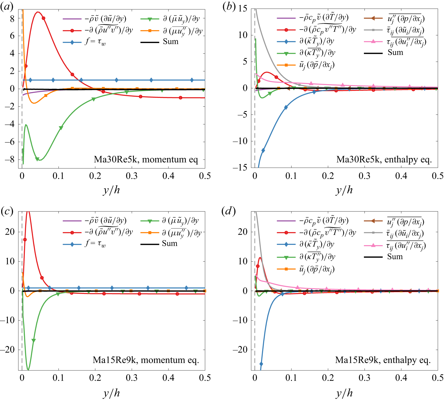
Figure 19. Mean-flow budgets of the (a,c) streamwise momentum equation (normalised by
 $\tau _w$
) and (b,d) enthalpy equation (normalised by
$\tau _w$
) and (b,d) enthalpy equation (normalised by
 $\vartheta _w$
) for cases (a,b) Ma30Re5k and (c,d) Ma15Re9k.
$\vartheta _w$
) for cases (a,b) Ma30Re5k and (c,d) Ma15Re9k.
Appendix C. Derivation for the shapes of acoustic modes
For a uniform inviscid free
stream
 $[\bar {\rho },\,\tilde {u},\,0,\,0,\,\tilde {T}]^{T}$
, the linear operator has four eigenmodes
$[\bar {\rho },\,\tilde {u},\,0,\,0,\,\tilde {T}]^{T}$
, the linear operator has four eigenmodes
 $\mathcal{L}_q\,\check {\!\boldsymbol q}^{{\prime \prime }}=-{\mathrm{i}}\omega \,\check {\!\boldsymbol q}^{{\prime \prime }}$
, related to vortical modes, slow and fast acoustic modes and entropy modes, respectively. The eigenvalues of slow and fast acoustic modes are
$\mathcal{L}_q\,\check {\!\boldsymbol q}^{{\prime \prime }}=-{\mathrm{i}}\omega \,\check {\!\boldsymbol q}^{{\prime \prime }}$
, related to vortical modes, slow and fast acoustic modes and entropy modes, respectively. The eigenvalues of slow and fast acoustic modes are
 $\omega =k_x\tilde {u}\pm |{\boldsymbol k}|a$
, and their eigenfunctions (
$\omega =k_x\tilde {u}\pm |{\boldsymbol k}|a$
, and their eigenfunctions (
 ${\boldsymbol q}^{{\prime \prime }}=\,\check {\!\boldsymbol q}^{{\prime \prime }}\exp [{\mathrm{i}}(k_xx+k_yy+k_zz)]$
) take the form
${\boldsymbol q}^{{\prime \prime }}=\,\check {\!\boldsymbol q}^{{\prime \prime }}\exp [{\mathrm{i}}(k_xx+k_yy+k_zz)]$
) take the form
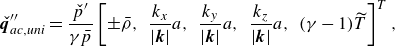 \begin{equation} \,\check {\!\boldsymbol q}_{\textit {ac},\textit {uni}}^{{\prime \prime }} = \frac {\check {p}^{\prime }}{\gamma \bar {p}} \left [ \pm \bar {\rho },\,\, \frac {k_x}{|{\boldsymbol k}|}a,\,\, \frac {k_y}{|{\boldsymbol k}|}a,\,\, \frac {k_z}{|{\boldsymbol k}|}a,\,\, (\gamma -1)\widetilde {T} \right ]^{T}, \end{equation}
where
 $k_y$
is a virtual wall-normal wavenumber and
$k_y$
is a virtual wall-normal wavenumber and
 $|{\boldsymbol k}|^2=k_x^2+k_y^2+k_z^2$
. In the presence of channel walls, the boundary condition requires
$|{\boldsymbol k}|^2=k_x^2+k_y^2+k_z^2$
. In the presence of channel walls, the boundary condition requires
 $\check {v}=0$
at
$\check {v}=0$
at
 $y=0,2h$
, so
$y=0,2h$
, so
 $\check {v}\!\sim \!{\mathrm{i}}\sin (n\pi y/2h)$
and
$\check {v}\!\sim \!{\mathrm{i}}\sin (n\pi y/2h)$
and
 $\check {u},\check {w},\check {\rho },\check {T},\check {p}\!\sim \!\cos (n\pi y/2h)$
, where
$\check {u},\check {w},\check {\rho },\check {T},\check {p}\!\sim \!\cos (n\pi y/2h)$
, where
 $n=0,1,2,\ldots$
. As a result, the eigenfunction (
$n=0,1,2,\ldots$
. As a result, the eigenfunction (
 ${\boldsymbol q}^{{\prime \prime }}=\,\check {\!\boldsymbol q}^{{\prime \prime }}(y)\exp [{\mathrm{i}}(k_xx+k_zz)]$
), as in (5.3), is expressed as
${\boldsymbol q}^{{\prime \prime }}=\,\check {\!\boldsymbol q}^{{\prime \prime }}(y)\exp [{\mathrm{i}}(k_xx+k_zz)]$
), as in (5.3), is expressed as
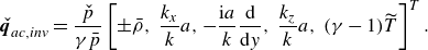 \begin{equation} \,\check {\!\boldsymbol q}_{\textit {ac},\textit {inv}} = \frac {\check {p}}{\gamma \bar {p}} \left [ \pm \bar {\rho },\,\frac {k_x}{k}a,-\frac {{\mathrm{i}} a}{k}\frac {{{\rm d}}}{{{\rm d}} y},\,\frac {k_z}{k}a,\,(\gamma -1)\widetilde {T} \right ]^{T}. \end{equation}
Note that
 $n=0$
is further adopted in (C2). This lowest-order mode was shown to contain the highest energy compared with other higher-order modes because its eigenvalue is the closest to the vortical and entropy modes in the eigen-spectrum (e.g. Chen et al. Reference Cheng and Fu2023b
). Although the wall-normal variation of the mean flow is not considered in deriving the analytical (C2), this simple relation will be shown to be highly accurate in most wall-normal regions.
$n=0$
is further adopted in (C2). This lowest-order mode was shown to contain the highest energy compared with other higher-order modes because its eigenvalue is the closest to the vortical and entropy modes in the eigen-spectrum (e.g. Chen et al. Reference Cheng and Fu2023b
). Although the wall-normal variation of the mean flow is not considered in deriving the analytical (C2), this simple relation will be shown to be highly accurate in most wall-normal regions.
Equation (C2) is not compatible with the viscous wall boundary which is no slip and isothermal. This inconsistency leads to non-zero
 $\check {u}_{i,w}^{{\prime \prime }}$
,
$\check {u}_{i,w}^{{\prime \prime }}$
,
 $\check {w}_{i,w}^{{\prime \prime }}$
and
$\check {w}_{i,w}^{{\prime \prime }}$
and
 $\check {T}_w^{{\prime \prime }}$
for
$\check {T}_w^{{\prime \prime }}$
for
 $\langle \hat {\boldsymbol q}^{{\kern0.3pt}{\prime \prime }} \hat {\boldsymbol q}^{{{\prime \prime }}{{H}}} \rangle _{\textit {nac}}$
, which can disrupt the decomposition of the forcing based on the full NS operator. To solve this problem, an acoustic boundary layer is required. Learning from Pierce (Reference Pierce2019, chapter 10), a simple exponential profile is assumed within the boundary layer to damp the finite
$\langle \hat {\boldsymbol q}^{{\kern0.3pt}{\prime \prime }} \hat {\boldsymbol q}^{{{\prime \prime }}{{H}}} \rangle _{\textit {nac}}$
, which can disrupt the decomposition of the forcing based on the full NS operator. To solve this problem, an acoustic boundary layer is required. Learning from Pierce (Reference Pierce2019, chapter 10), a simple exponential profile is assumed within the boundary layer to damp the finite
 $\check {u}_{i}^{{\prime \prime }}$
and
$\check {u}_{i}^{{\prime \prime }}$
and
 $\check {T}^{{\prime \prime }}$
to zero at the wall. The damping function, applied to
$\check {T}^{{\prime \prime }}$
to zero at the wall. The damping function, applied to
 $\check {u}^{{\prime \prime }}$
,
$\check {u}^{{\prime \prime }}$
,
 $\check {w}^{{\prime \prime }}$
and
$\check {w}^{{\prime \prime }}$
and
 $\check {T}^{{\prime \prime }}$
, is
$\check {T}^{{\prime \prime }}$
, is
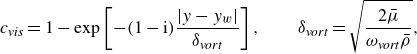 \begin{equation} c_{\textit {vis}} = 1 - \exp \left [-(1-{\mathrm{i}})\frac {|y-y_w|}{\delta _{\textit {vort}}}\right ], \qquad \delta _{\textit {vort}} = \sqrt {\frac {2\,\bar {\!\mu }}{\omega _{\textit {vort}}\bar {\rho }}}, \end{equation}
where
 $\delta _{\textit {vort}}$
is a characteristic boundary layer thickness, and the frequency of vortical modes is approximated as
$\delta _{\textit {vort}}$
is a characteristic boundary layer thickness, and the frequency of vortical modes is approximated as
 $\omega _{\textit {vort}}\approx k_xU_b$
. The introduction of (C3) finally leads to the viscous relation in (5.3).
$\omega _{\textit {vort}}\approx k_xU_b$
. The introduction of (C3) finally leads to the viscous relation in (5.3).

Figure 20. Eigenfunctions (normalised by the energy norm) of the leading fast acoustic mode for fluctuations of (a,b)
 $(\lambda _x,\lambda _z)/h=(12.6,1.3)$
with
$(\lambda _x,\lambda _z)/h=(12.6,1.3)$
with
 $\omega h/U_b\approx 3.1$
and (c,d)
$\omega h/U_b\approx 3.1$
and (c,d)
 $(\lambda _x,\lambda _z)/h=(0.6,6.3)$
with
$(\lambda _x,\lambda _z)/h=(0.6,6.3)$
with
 $\omega h/U_b\approx 17.5$
for case Ma30Re5k: (a,c) pressure from both the inviscid and viscous linear operators, and (b,d) the components from the viscous linear operator and from (5.3).
$\omega h/U_b\approx 17.5$
for case Ma30Re5k: (a,c) pressure from both the inviscid and viscous linear operators, and (b,d) the components from the viscous linear operator and from (5.3).
Equation (5.3) is examined in figure 20 for two sets of wavenumbers as in figure 17. Here, the eigenfunctions of the leading fast acoustic mode are displayed, which is selected from the eigen-spectrum of
 $\mathcal{L}_q$
with the minimum
$\mathcal{L}_q$
with the minimum
 $|\omega |\approx k_x\tilde {u}_c+ka_c$
. The results for slow acoustic modes are quantitatively similar. Figures 20(a) and 20(c) demonstrate that including viscosity or not in
$|\omega |\approx k_x\tilde {u}_c+ka_c$
. The results for slow acoustic modes are quantitatively similar. Figures 20(a) and 20(c) demonstrate that including viscosity or not in
 $\mathcal{L}_q$
negligibly affects the shape function of
$\mathcal{L}_q$
negligibly affects the shape function of
 $\check {p}^\prime$
, validating the additional formulation of the acoustic boundary layer. The shape functions of velocity, density and temperature from
$\check {p}^\prime$
, validating the additional formulation of the acoustic boundary layer. The shape functions of velocity, density and temperature from
 $\mathcal{L}_q$
, and from (5.3) and
$\mathcal{L}_q$
, and from (5.3) and
 $\check {p}^{\prime }$
, are compared in figures 20(b) and 20(d). Equation (5.3) is shown to estimate well all the five components of
$\check {p}^{\prime }$
, are compared in figures 20(b) and 20(d). Equation (5.3) is shown to estimate well all the five components of
 $\,\check {\!\boldsymbol q}^{{\prime \prime }}$
in the outer layer for different
$\,\check {\!\boldsymbol q}^{{\prime \prime }}$
in the outer layer for different
 $(\lambda _x,\lambda _z)$
. Using (C3) leads to slightly larger deviations near the wall, but it does not deteriorate the evaluation of
$(\lambda _x,\lambda _z)$
. Using (C3) leads to slightly larger deviations near the wall, but it does not deteriorate the evaluation of
 $\langle \hat {\boldsymbol q}^{{\kern0.3pt}{\prime \prime }} \hat {\boldsymbol q}^{{{\prime \prime }}{{H}}} \rangle _{\textit {ac}}$
in § 5.2.
$\langle \hat {\boldsymbol q}^{{\kern0.3pt}{\prime \prime }} \hat {\boldsymbol q}^{{{\prime \prime }}{{H}}} \rangle _{\textit {ac}}$
in § 5.2.


 Open access