


1. Introduction
The ability to learn the relations between causes and effects is critical for decision-making. However, assessing the influence of any individual cause on an effect requires accounting for other confounded causes. For example, when judging how a new medication affects sleep, one should also consider other variables that affect the probability of sleeping well (e.g., stress, alcohol, caffeine, and exercise). The current research is focused on how people account for confounded causes when assessing cause–effect relations from observed events, analogously to how a statistician uses multiple regression to account for alternative predictors.
Accounting for alternative causes, known as ‘credit assignment’, is fundamental to fields that study intelligent and adaptive behavior and judgment. In the field of associative learning, credit assignment drove the production of the Rescorla and Wagner (Reference Rescorla, Wagner, Black and Prokasy1972) model and other models of associative learning (Luzardo et al., Reference Luzardo, Alonso and Mondragón2017; Pearce and Hall, Reference Pearce and Hall1980) based on findings of cue competition in animal learning (e.g., Kamin, Reference Kamin and Jones1968). Cue competition involves paradigms in which the participant is simultaneously learning about two or more cues that may be correlated with each other. Cue competition includes many different paradigms, including forward blocking (Chapman and Robbins, Reference Chapman and Robbins1990; Dickinson et al., Reference Dickinson, Shanks and Evenden1984; Wasserman, Reference Wasserman1990), backward blocking (Kruschke and Blair, Reference Kruschke and Blair2000; Shanks, Reference Shanks1985; Wasserman and Berglan, Reference Wasserman and Berglan1998), overshadowing (De Houwer et al., Reference De Houwer, Vandorpe and Beckers2005; Mackintosh, Reference Mackintosh1976; Price and Yates, Reference Price and Yates1993), and un-overshadowing (Larkin et al., Reference Larkin, Aitken and Dickinson1998). Subsequent reinforcement-learning models were designed to accomplish a similar goal of credit assignment (e.g., Gallistel et al., Reference Gallistel, Craig and Shahan2019; Sutton and Barto, Reference Sutton and Barto2018), which have made important contributions to neuroscience (see Stolyarova, Reference Stolyarova2018, for a review).
In the causal learning literature, there is considerable evidence that people can control for alternative causes when judging the strength of a target cause (see Rottman, Reference Rottman and Waldmann2017, for a review). However, there is also evidence for a non-normative behavior called discounting; when learning about two potential causes of an effect, if one cause has a stronger relation with the effect, then the stronger cause tends to overshadow the weaker one and people devalue the perceived efficacy of the weaker cause in a contrasting way (Busemeyer et al., Reference Busemeyer, Myung and McDaniel1993; Goedert et al., Reference Goedert, Harsch and Spellman2005; Goedert and Spellman, Reference Goedert and Spellman2005; Laux et al., Reference Laux, Goedert and Markman2010). Specifically, if there is one strongly positive cause and one weakly positive cause, people tend to give weaker ratings for the weak cause, compared to if both causes are weak.
The major contribution of the current study is to test whether people can accurately assess cause–effect relations and account for alternative causes in more realistic settings, particularly in learning settings that are extended over time. Prior research has been conducted with data presented over a rapid sequence of back-to-back trials with minimal distractions. However, most learning takes place over longer periods of time; for example, learning about the effectiveness or side effects of a new medication could take weeks or even months. In the current research a smartphone application was developed to study controlling for alternative causes and discounting in a more realistic timeframe in which learning unfolds over weeks (1 trial per day for 24 days) as opposed to observing back-to-back trials.
1.1. Psychological theories of controlling and evidence
When doing statistics, a researcher can choose to conduct an unconditional analysis that examines the simple relation between two variables, or a conditional analysis that examines the relation between two variables while controlling for one or more other variables. Controlling for a third variable when assessing the influence of a target cause on an effect is normative if the learner thinks that the third variable could also cause the effect. Unconditional versus conditional assessments of a cause–effect relation can differ by only a little bit or can differ considerably. An extreme version is called Simpson’s paradox, in which the unconditional relation is positive, but the conditional relation is negative, or vice versa (see Kievit et al., Reference Kievit, Frankenhuis, Waldorp and Borsboom2013, for a review).
There are a number of theories of how people could control for third variables. One theory is called ‘focal sets’ (Cheng, Reference Cheng1997; Cheng and Novick, Reference Cheng and Novick1992). For example, consider the ΔP rule (Allan, Reference Allan1980), a model that calculates unconditional causal strength as the difference between the probability of effect E occurring in the presence (1) and absence (0) of target cause T (Equation (1)). It is possible to use ΔP and control for an alternative cause A by calculating ΔP within the subset in which A is present (a = 1; Equation (2)), or absent (a = 0; Equation (3)), which have been termed ‘focal sets’ (Cheng, Reference Cheng1997; Cheng and Novick, Reference Cheng and Novick1992). One challenge is that Equations (2) and (3) could produce different estimates, although, in this study, the learning data were chosen such that they produce the same estimates. Another challenge with focal set theory is that it provides an unsatisfactory explanation for learning about many causes; with n binary causes, there will be 2 n − 1 focal sets to choose from, and each one may have very few observations (Derringer and Rottman, Reference Derringer and Rottman2018).
 $$\begin{align}{\Delta P}_T&=p\left(e=1|t=1\right)-p\left(e=1|t=0\right).\end{align}$$
 $$\begin{align}{\Delta P}_{T,a=1}&=p\left(e=1|t=1,a=1\right)-p\left(e=1|t=0,a=1\right).\end{align}$$
 $$\begin{align}{\Delta P}_{T,a=0}&=p\left(e=1|t=1,a=0\right)-p\left(e=1|t=0,a=0\right).\end{align}$$
Multiple regression accomplishes a similar goal to conditional ΔP but can handle more causes and can handle metric (as opposed to just binary) variables. Psychologists have long used multiple regression or ANOVA as a computational-level account of human causal inference (e.g., Kelley, Reference Kelley, Jones, Kanounse, Kelley, Nissbett, Valins and Weiner1972).
A third class of theories of controlling for third variables is reinforcement-learning and associative-learning models. Stone (Reference Stone, Rumelhart and McClelland1986) proved that the delta rule, which underlies many such models, is an iterative method for computing multiple linear regression coefficients. The experiments reported here were not designed to test for differences in these theories; all standard approaches will make similar predictions.
1.2. Controlling for alternative causes in prior research
A variety of studies have found that, at least in some conditions, people are able to control for alternative causes. In Spellman (Reference Spellman1996), three groups of participants learned about two liquids that could potentially generate, inhibit, or have no effect on plant growth. In each trial, participants observed whether a plant did or did not receive each liquid and whether the plant bloomed or did not bloom. In one experiment, the unconditional strength of the target was held constant, but its conditional strength varied across the three groups; assessments of the target varied in the same direction as conditional strength. In the other experiment, the unconditional strength of the target varied, but its conditional strength was held constant; there were no differences in judgments for the target across the three groups. Together, these findings show that people can and will control for other cues by conditionalizing on the alternative.
There is additional evidence that people will selectively control for what they perceive to be causally relevant cues (Goodie et al., Reference Goodie, Williams and Crooks2003; Waldmann, Reference Waldmann2000; Waldmann and Hagmayer, Reference Waldmann and Hagmayer2001; Waldmann and Holyoak, Reference Waldmann and Holyoak1992), which is also rational, given that one should only control for variables they think plausible alternative causes of the effect. Spellman (Reference Spellman1996) cited controlling for alternative causes as evidence for people ‘acting as intuitive scientists’ because it is a central tenet of research methodology. There is also evidence that some skills necessary for controlling develop quite early, and that 3-year-old (Schulz and Gopnik, Reference Schulz and Gopnik2004) and sometimes 2-year-old (Gopnik et al., Reference Gopnik, Sobel, Schulz and Glymour2001) children can use covariation information to make causal inferences.
Derringer and Rottman (Reference Derringer and Rottman2018) conducted a study that is particularly relevant to the current research. In this study, participants learned about eight causes simultaneously, and after each learning trial, they updated their causal strength beliefs about the eight causes. The trial-by-trial updates were compared to the Rescorla–Wagner model and to running a multiple regression after each trial. We found some similarities to both of these approaches; however, the clearest finding was that participants were most likely to update their belief about a given cause when that cause changed from absent to present, and the other causes remained stable, which we termed ‘informative transitions’. For example, suppose that on Monday, you are stressed, do not exercise, and sleep poorly, and then on Tuesday, you are still stressed, do exercise, and sleep well. Because being stressed was constant across Monday and Tuesday, and exercise changed and sleep changed, you might view this comparison between two adjacent days to be especially informative for assessing if exercise improves sleep. In contrast, if both exercise and stress changed from one day to the next, it could be difficult to assess if either is responsible for the change in sleep.
A number of other studies from my lab suggest that when learning cause–effect relations, people tend to learn from the changes in the cause and effect rather than or in addition to the presence versus absence of the cause and effect (e.g., Rottman, Reference Rottman2016; Rottman and Keil, Reference Rottman and Keil2012; Soo and Rottman, Reference Soo and Rottman2018).Footnote 1 This theory of informative transitions makes a prediction about learning in long-timeframe scenarios, which will be explained below.
1.3. Discounting in prior research
Controlling for alternative causes is a rational way of addressing the problem of credit assignment; however, there is also considerable evidence of a non-rational process called ‘discounting’. When one cause is considerably stronger than the other, participants tend to ‘discount’ or devalue the strength of the weaker cause (Baetu and Baker, Reference Baetu and Baker2019; Busemeyer et al., Reference Busemeyer, Myung and McDaniel1993; Dickinson et al., Reference Dickinson, Shanks and Evenden1984; Goedert et al., Reference Goedert, Harsch and Spellman2005; Goedert and Spellman, Reference Goedert and Spellman2005; Laux et al., Reference Laux, Goedert and Markman2010). Another way to explain this is that the stronger cause has a contrastive effect on the assessment of the weaker cause. Goedert and Spellman (Reference Goedert and Spellman2005) found that participants gave weaker judgments for the target when the alternative was stronger than when the alternative was weak. The contrasting effect of the alternative on judgments for the target is evidence of non-normative discounting.
1.4. Learning over long timeframes
The primary goal of the current research was to study participants’ ability to learn about two correlated causes over a longer, more realistic, timeframe. The timing of the standard trial-by-trial paradigm is artificial in that the trials are presented very rapidly. I contend that many if not most real-world inferences are made from experiences spanning days, weeks, or even months, and therefore it is vital to understand how well people can control for alternative causes in a more realistic setting.
My lab has recently developed a paradigm that we call ‘ecological momentary experiments’ in which participants experience one piece of evidence about the cause–effect relation each day over many days. (The name is meant as building upon ‘ecological momentary assessments’, in which responses are collected from participants periodically during their daily lives, e.g., Shiffman et al., Reference Shiffman, Stone and Hufford2008.) This paradigm is meant to mimic many real-life situations that involve learning about causes and effects in one’s life such as learning about the efficacy of medications or lifestyle choices (see also Wimmer et al., Reference Wimmer, Li, Gorgolewski and Poldrack2018, and Mack et al., Reference Mack, Cinel, Davies, Harding and Ward2017, for similar paradigms for studies on reinforcement learning and memory). In one study, we found that participants accurately learned about single cause–effect relations when the cause and effect were correlated, similar to in the short timeframe. Additionally, the participants exhibited illusory correlation in the long timeframe similar to the short timeframe—they believed that the cause and effect were related even when they were not (Willett and Rottman, Reference Willett and Rottman2021).
In another study, we investigated interrupted time series situations in which a cause is absent for multiple days and then present for multiple days, and the effect can exhibit a change in level or slope after the cause starts. Although we found that participants made poor judgments in certain situations, their judgments were similar between the short and long timeframes with fairly subtle differences (Zhang and Rottman, Reference Zhang and Rottman2023).
In a third study, we tested whether people can accurately learn cause–effect relations when the experiences are spaced out over days and when there are hours-long delays between the cause-and-effect events (Zhang and Rottman, Reference Zhang and Rottman2024). We found some evidence that learning was slowed with longer delays, but by the end of 16 days, participants had learned the cause–effect relation about equally well, with delays of 0, 3, 9, and 21 hours. In sum, although we have found some evidence of differences in causal learning between the short and long timeframes, these differences have been subtle, and largely we have found similar learning.
1.5. The impact of timeframe on learning about two causes
To date, all of the studies on causal learning over a long timeframe have involved only a single cause and effect. The goal of the current study was to assess whether there are differences in people’s ability to control for alternative causes in long compared to short timeframes, and more importantly, whether people can accurately control for alternative causes in a long timeframe. There are at least two reasons that causal learning over long timeframes may be harder with more complex situations such as when there are two or more causes.
First, at a general level, there is some evidence that increased demand on working memory can impede the ability to control for alternative causes (Goedert et al., Reference Goedert, Harsch and Spellman2005) and reduce non-normative discounting (De Houwer et al., Reference De Houwer, Vandorpe and Beckers2005; Goedert and Spellman, Reference Goedert and Spellman2005). In Goedert et al. (Reference Goedert, Harsch and Spellman2005), participants completed either a verbal or spatial working memory task while simultaneously learning about two causes and an effect; the verbal task reduced controlling, and the spatial task reduced discounting. Using a forward blocking paradigm, De Houwer and Beckers (Reference De Houwer and Beckers2003) found reduced blocking when participants simultaneously performed a difficult versus an easy secondary task. If the long timeframe is more taxing on memory resources, it may produce both reduced controlling and reduced discounting in the long timeframe. However, given that the prior research on single cause–effect learning has not shown that learning is considerably harder in the long timeframe, this may not occur for two causes either.
Second, the informative transitions theory (Derringer and Rottman, Reference Derringer and Rottman2018) predicts that learning in a long timeframe may be particularly hard. As a reminder, this theory proposes that people primarily update their beliefs about a given cause when that cause changes and when the other cause(s) remain stable. In the previous example about being stressed for 2 days in a row, but only exercising on the second day and sleeping better on the second day, the informative transitions theory requires the learner to remember all the events that happened the prior day (stress, no exercise, and poor sleep) and compare them to what happened the current day. These changes are likely less salient, or potentially more effortful to recall, when the events occur on successive days than when the trials are presented in short succession.Footnote 2 In contrast, we have argued that in short timeframe situations when the cues are presented adjacent to each other, the changes are perhaps even more salient than the states of the variables.
It is possible that the changes will still be fairly salient in the long-timeframe environment. However, if the changes are less salient in the long timeframe, there are a few possibilities for what might happen. First, if people rely on informative transitions for causal learning but cannot use them in the long timeframe, then their learning may be quite bad in the long timeframe; they may simply feel uncertain about the causal relations. Second, learners might instead resort to a standard reinforcement-learning process similar to Rescorla and Wagner (Reference Rescorla, Wagner, Black and Prokasy1972), in which only the events during the current moment need to be attended to, not the changes from the events the prior day. In this case, learners would still be able to control for the alternative cause. Third, people could resort to learning the simple bivariate (unconditional) cause–effect relations instead of controlling for the alternative cause.
Although Derringer and Rottman (Reference Derringer and Rottman2018) provided clear evidence that people primarily focus on changes in causes, it is also possible that this finding may not generalize to the current study. Focusing on changes is especially cognitively efficient when most causes remain fairly stable and when there are many causes (see footnote 2). Derringer and Rottman still found that people focused on changes when the learning data were randomly ordered, but more so when the learning data were autocorrelated. However, in the current study, the participants only learned about two causes, and the learning data were randomly ordered. Both of these decisions were chosen to replicate Spellman (Reference Spellman1996). But it could also mean that people in both the short and long timeframes learn by focusing more on presence versus absence and not on changes, in which case there may not be many differences between the short and long timeframes.
In sum, there are a variety of potential outcomes. The goal for this research was not to test a particular theoretical account, as there are simply too many possibilities, and there is such little research on learning in long-timeframe environments that there are not yet clear theoretical accounts about the roles of memory and salience of events. Instead, the primary goal was to assess how accurately people control for alternative causes in the long timeframe. This question is of utmost importance as it can provide guidance about whether or not individuals can trust their own causal conclusions formed from everyday learning.
1.6. The current research
As just explained, the primary goal was to assess how accurately people control for alternative causes in the long timeframe. A secondary goal was to test for differences in controlling between the long and short timeframes, which can provide guidance into theorizing about the learning processes that occur in long-timeframe learning.
In addition to testing controlling, the paradigm being used, similar to Spellman’s (Reference Spellman1996) study, also allows for two other assessments of causal learning and judgment. First, this paradigm tests for ‘simple learning’—learning about a cue that has a similar unconditional and conditional strength on an outcome. For many of the same reasons mentioned above about controlling, if it is hard for people to learn the cause–effect relations between two causes and an effect in a long-timeframe situation, then their ability to learn even about cues that have a simple relation with an effect may also be impaired when there is a second cause. This paradigm also tests for non-normative discounting, whether a strong cue has a contrasting impact on the judged strength of another cue. This is the first time that simple learning and non-normative discounting are being tested in a long-timeframe learning situation, and the short and long timeframes will also be compared.
Because of the possibility of order effects in Experiment 1, a second experiment was conducted that only tested the long-timeframe condition so that there could be no order effects. This study allowed for considerably greater power to examine learning in the long timeframe.
2. Experiment 1
2.1. Methods
2.1.1. Participants
A total of 205 participants were recruited for the study; the main requirements were owning a smartphone and intending to complete the 25-day study. Participants were paid $30 if they completed the entire study. Of the 200 participants who completed the study, 191 were included in the final analyses, after excluding 1 person due to potential confusion with the task (because they were not fluent in English) and 8 people due to an error in data collection.
The mean age was 22.10 years (SD = 7.34), and the 5th and 95th percentiles were 18 and 30 years. With regard to sex, 72% identified as female, 27% as male, and 1% as non-binary. With regard to ethnicity, 7% reported being Hispanic or Latino, 88% not, and 5% did not report. With regard to race, for which participants could select more than one, 1% identified as American Indian or Alaska Native, 25% as Asian, 7% as Black or African American, 0% as Native Hawaiian or Other Pacific Islander, 66% as White, and 5% did not report. Lastly, 79% were undergraduate students, 11% were graduate students, and 10% were not currently students.
2.1.2. Cover story
In the cover story, participants were asked to learn about two medicines, which could improve, worsen, or have no influence on insomnia.Footnote 3 (Participants did not actually take medicines—the entire task is imaginary.) The task was an observational causal learning task; participants did not choose to use the medicines on each day or not, but instead were told which medications they used on a given day. The task was introduced with the following text:
Please imagine that you have chronic insomnia. Due to two other health conditions you have, you are on two medications Allapan and Worfen, to treat these conditions.
You have heard that sometimes other medications can improve or worsen insomnia as a side effect. Some medications happen to improve insomnia as a side effect by making you feel more tired before going to bed and helping you stay asleep throughout the night. Other medications happen to worsen insomnia as a side effect by making you agitated and awake at night.
You want to figure out whether Allapan and/or Worfen each improve or worsen or have no influence on your insomnia….
Note: It is possible that both medicines improve your insomnia, or both medicines worsen your insomnia, or one improves and the other worsens your insomnia, or each one might also have no effect on your insomnia….
2.1.3. Stimuli and design
Participants were randomly assigned to learn about one of four datasets (adapted from Spellman, Reference Spellman1996), defined by whether the T and the A each have a generative or preventative conditional influence on the effect. For example, in the TgenAgen dataset, T has a generative conditional influence on the effect, and A also has a generative conditional influence on the effect. See Table 1 for summary statistics, Table 2 for event frequencies, and Appendix A of the Supplementary Material for alternative ways of calculating unconditional and conditional strengths. The terminology used to name the ‘Target’ and ‘Alternate’ causes is only used to distinguish them in this paper, as has been done previously (Goedert and Spellman, Reference Goedert and Spellman2005; Laux et al., Reference Laux, Goedert and Markman2010); the instructions in the task did not imply a difference to participants.
Table 1 Conditional and unconditional ΔP for the four conditions
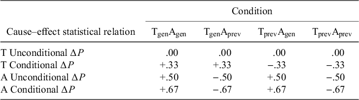
Note: A = alternative; T = target.
Table 2 Number of trials for each of eight event types across the four conditions

Note: 0 = absent; 1 = present; A = alternative; E = effect; T = target.
2.1.3.1. Controlling
The unconditional strength of T was always equal to zero, but the conditional strength of T was either generative (+.33) or preventative (−.33). This means that if participants do not control for A, judgments for T should be close to 0 in all four conditions. Alternatively, if participants do control for A, judgments for T should be more positive in the Tgen conditions than in the Tprev conditions, controlling for A. Unlike Spellman (Reference Spellman1996), the TgenAprev and TprevAprev conditions were included to obtain evidence of controlling when A has both generative and preventative influences.
2.1.3.2. Simple learning
The absolute values of the unconditional and conditional strengths of A on the effect were qualitatively the same across all four datasets. For example, in the TgenAgen condition, the unconditional influence of A is +.50, and the conditional influence is +.67. This means that if participants can learn about the alternative at all, regardless of whether they do or do not control for T, they should infer a generative relation for the Agen datasets and a preventative relation for the Aprev datasets. Because they do not need to control for T when assessing A, and because A is stronger than T, it should be easier to learn about A.
2.1.3.3. Non-normative discounting
This design also allowed us to test for non-normative discounting. Evidence that people discount T in comparison to A would appear as a negative influence of A, controlling for T, when judging T. Likewise, evidence that people discount A in comparison to T would appear as a negative influence of T, controlling for A, when judging A. Because A is stronger than T in both conditional and unconditional strengths, it would be more likely to find that people discount T in comparison to A rather than the reverse.
2.1.3.4. Overall design
Participants completed the learning task in a short-term (back-to-back trials) format and a long-term (one trial per day) format using the same dataset and were randomly assigned to complete either the short or the long task first. Thus, the design was a 2 (timeframe: short vs. long, within-subjects) × 2 (T conditional strength: generative vs. preventative, between-subjects) × 2 (A conditional strength: generative vs. preventative, between-subjects).
2.1.4. Overall Procedure
Participants completed the study using their personal smartphones to access the website, which was run using the PsychCloud.org framework (Rottman, Reference Rottman2025 ). The study lasted 25 days, and the first and last days were completed in the lab.
On Day 1, participants completed an eight-trial practice task in which they learned about two causes simultaneously, one cause that was deterministic (ΔP = 1) and another cause that was non-contingent (ΔP = 0). The purpose of the practice task was to acclimate participants to the trial-by-trial procedure before completing the short and long tasks. After the practice task, participants assigned to the short-task-first condition completed the short task, whereas participants assigned to the long-task-first condition proceeded directly to the long task. To complete Day 1, each participant completed Trial 1 of the long task. On Days 1–24, participants logged in to complete the daily trial for the long task and received text message reminders at 10 am, 3 pm, and 8 pm if they had not yet completed the trial each day. On Day 25, participants returned to the lab to complete the dependent measures for the long task. Participants in the long-task-first condition then completed the short task. After completing the tasks, participants were paid and debriefed.
All three tasks involved learning about two medicines. The names, shapes, and colors of the medicines were all different. For the practice task, the effect was arthritis pain. For the short and long-timeframe tasks, the effects—dizziness and insomnia—were randomized. The instructions stated that the medicines could improve, worsen, or have no influence on the effect and that the goal was to infer the influence of each medicine on the effect.
Participants were told that if they missed more than 3 days of the study, the study would be terminated. If participants missed 1 day (7%), 2 days (3%), or 3 days (1%) of the study, the subsequent trials were pushed back so that they experienced each trial on a different day. Most participants returned to the lab 1 day after completing Trial 24 (90%), but some returned on the same day (9%), or 2 days later (1%).
2.1.5. Procedure Within a trial
Across the short- and long-timeframe tasks, each trial followed the same procedure with four steps. First, participants saw text and icons that depicted whether T and A were each present or absent on that trial (Figure 1a). To proceed, participants pressed radio buttons to verify the state of each cause. Second, having learned the state of both causes, participants pressed a radio button to predict whether the effect would be present or absent and then pressed a submit button to proceed (Figure 1b). Third, they were given feedback about their prediction (Correct/Incorrect) and saw text and an icon that depicted the true state of the effect. To proceed, participants pressed a radio button to verify the state of the effect (Figure 1c). Fourth, participants were instructed to ‘Imagine the scene until the images blink and the submit button appears’ to give them time to encode the information. After 4 seconds, the submit button appeared and participants pressed it to complete the trial. In the practice task and the short task, participants immediately proceeded to the next trial. In the long-timeframe condition, participants were logged out and unable to observe the next trial until the following day. At all points during the study, participants were unable to go back and see what happened on a prior trial.
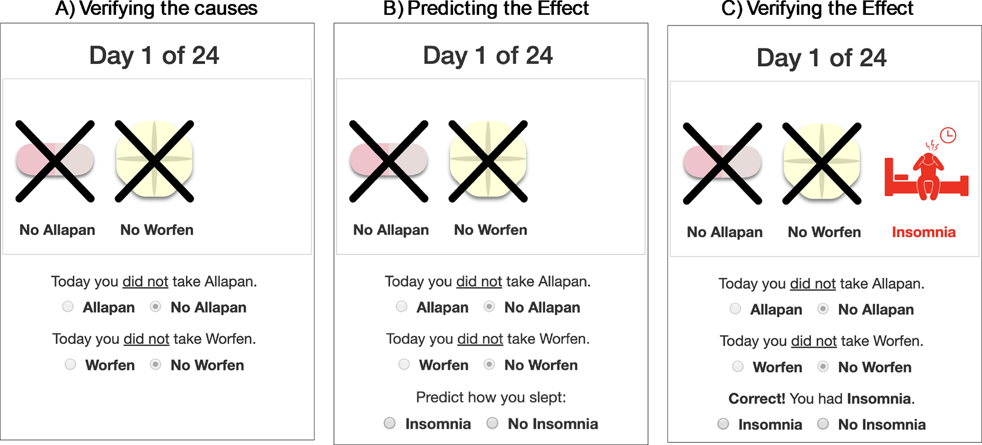
Figure 1 Screenshots of a single trial. (a) Participants were shown whether each of the two causes was present or absent and verified that they saw this information with radial buttons. (b) Participants predicted whether the effect would be present or absent. (c) Participants were shown if the effect was present or absent and verified this information with radial buttons.
2.1.6. Dependent measures
Participants’ beliefs about the strength of each cause on the effect were evaluated in three ways. First, for each cause, participants made an explicit judgment of ‘causal strength’; some version of causal strength is the most common question asked in studies of causal learning. Causal strength was calculated from their responses to two questions for each cause. In the first question, they made a general judgment about whether the cause improved, worsened, or had no influence on the effect. If they said ‘improved’ or ‘worsened’, they answered a second question about how strongly the cause improved/worsened the effect on a scale of 1–10. If they said ‘no influence’, participants skipped the second question and were assigned a judgment of 0. These responses were combined and mapped onto a −1 to +1 scale, where a judgment of −1 meant that the medicine always prevented the effect (i.e., improved symptoms), and a judgment of +1 meant that the medicine always caused the effect (i.e., worsened symptoms). Participants made causal strength ratings after Trials 8, 16, and 24. In the long-timeframe conditions, the causal strength ratings were made on Days 9, 17, and 25, prior to the learning experiences on Days 9 and 17.
Second, a measure of ‘tallies’ was derived from participants’ memories for the number of times they experienced each of the eight event types (T = present/absent, A = present/absent, E = present/absent). For example, they would recall the number of trials (out of 24) in which Medication X was absent, Medication Y was present, and the effect was present. The reason for assessing tallies is that the most common theories of causal inference (e.g., Cheng, Reference Cheng1997; Griffiths and Tenenbaum, Reference Griffiths and Tenenbaum2005; Hattori and Oaksford, Reference Hattori and Oaksford2007) assume that people use tallies of the event types to mentally calculate causal strength. Thus, assessing participants’ memories of these tallies provides another way to explore this inference process. The eight questions were presented on separate pages in a randomized order, and participants could enter any number between 0 and 24 for each question. For each participant, a single measure of the influence of T on E while controlling for A was calculated from the tallies using the average of Equations (2) and (3). The analogous procedure was used to calculate the influence of A on E while controlling for T from the tallies.Footnote 4 In 1% of cases, only one of the two equations could be used because the denominator for the other was equal to zero. Participants only made the tally judgments after Trial 24.
Third, a measure called ‘predictions during learning’ was created from participants’ predictions about the presence or absence of the effect. This measure provides an assessment of learning during the learning process. Since reinforcement learning theories assume that learners spontaneously make predictions, this measure may be more intuitive than some others. The predictions during Trials 12–24 were used for this measure; the last 13 trials were used so that participants had enough time to learn the relations and that each participant had seen at least one of the necessary event types for the calculations.Footnote 5 This measure was computed using the average of Equations (2) and (3), where E was the participants’ predictions of the effect rather than the actual effect. If only Equations (2) and (3) could be calculated because the participant had not seen each event type in the last 13 trials, the one equation that could be calculated was used; this happened for 15.4% of participants.
2.2. Analysis plan
The study design and analysis plan were registered after data collection began but before any analysis (see https://osf.io/3dajq/ for the analysis plan, data, and analysis code). Data were analyzed using R. Bayes factors (BFs) were computed with the package BayesFactor. The BFs are presented in the odds format; 10 means that the alternate hypothesis is 10 times as likely as the null, and .10 means that the null is 10 times as likely as the alternate. The package effsize Torchiano, Marco (Reference Torchiano2020) was used to compute ηp 2 effect sizes; effect sizes are reported in the OSF registration rather than in the manuscript because they do not add very much in addition to the regression coefficients. The predictors were coded as +.5 for the generative conditional influence datasets and −.5 for preventative.
2.2.1. Order effects
As preregistered, preliminary analyses were conducted to test whether there are order effects, given that participants completed the same task in both the short and long timeframes. Appendix B of the Supplementary Material presents these findings; there appeared to be some order effects, but there were also many findings that did not reveal order effects. Notably, there were no order effects in the analyses of controlling, the most important analysis of this study.
For utmost caution, the between-subject analyses of only the first task that participants completed, either short or long, are reported in the main manuscript. In order to make as full use of the data as possible, the within-subject analyses of both tasks are reported in Appendix B of the Supplementary Material.
2.2.2. Statistical tests of controlling, simple learning, and discounting, within both the short and long timeframes
Two main regressions were run within both the short and long timeframes: predicting judgments about the target from T, whether the Target was generative or preventative, and from A, whether the Alternative was generative or preventative (Equations (4) and (5)). These two regressions produce four regression coefficients. The results from these regressions are reported in Table 3. The interpretation of each coefficient is captured in the superscripts in Equations (4) and (5), and is discussed next:
 $$\begin{align}\mathrm{Judgment}\kern0.17em \mathrm{of}\;\mathrm{T}\sim {\mathrm{T}}^{\mathrm{Controlling}}+{\mathrm{A}}^{\mathrm{Discounting}}.\end{align}$$
 $$\begin{align}\mathrm{Judgment}\kern0.17em \mathrm{of}\;\mathrm{A}\sim {\mathrm{A}}^{\mathrm{SimpleLearning}}+{\mathrm{T}}^{\mathrm{Discounting}}.\end{align}$$
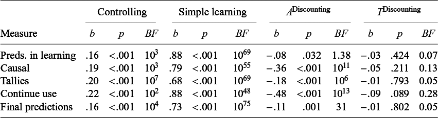
Table 3 Regression results for judgments in Experiment 1 analyzing only the first task
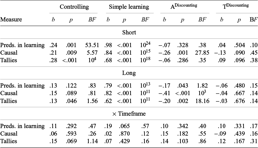
Note: BFs greater than 102 are rounded to the nearest exponent.
The coefficient for T in Equation (4) assesses whether participants give more positive judgments about T in the Tgen conditions than in the Tprev conditions. If this coefficient is positive, it is evidence of controlling because only a conditional assessment of T predicts this difference, not an unconditional assessment (rows 1 and 2 in Table 1). The coefficient for A in Equation (5) assesses whether participants give more positive judgments about A in the Agen conditions than in the Aprev conditions. If this coefficient is positive, it is evidence of simple learning because both a conditional assessment of A and an unconditional assessment of A predict this difference (rows 3 and 4 in Table 1).
The coefficient for A when judging T in Equation (4) and the coefficient for T when judging A in Equation (5) both assess non-normative discounting. In Table 1, notice that when assessing T in rows 1 and 2, there is no difference based on Agen versus Aprev; there should only be a difference in judgment based on the condition of T. Likewise, when assessing A in rows 3 and 4, there is no difference based on Tgen versus Tprev; there should only be a difference in judgments based on the condition of A. If ADiscounting and TDiscounting are negative, it would mean that these cues are having a discounting or contrasting impact on the strength of the other cue, even though they should have no impact. Previous research has found that typically the stronger cue discounts the weaker cue, but not necessarily the reverse, so it would make sense for ADiscounting in Equation (4) to be stronger than TDiscounting in Equation (5).
In addition to comparing the regression coefficients to 0, the weights for controlling and simple learning were also compared to their ideal values for the tally measure.Footnote 6 The ideal regression weight for controlling is b = .67, which is the difference in conditional strength for Tgen (+.33) and Tprev (−.33). The ideal regression weight for simple learning is b = 1.33, which is the difference in conditional strength of the Agen (.67) and Aprev (−.67) conditions.
2.2.3. Statistical tests assessing the impact of timeframe
The impact of timeframe on controlling, simple learning, and the two types of discounting was also assessed. For the analysis in which only the first learning experience was included (either short or long, between-subjects), the interactions between Timeframe and T, and between Timeframe and A (Equations (6) and (7)), were added to the regressions. For the analysis of both learning experiences (both short and long, within-subjects), we ran the same regressions and added a by-subject random intercept.Footnote 7 These interactions are reported in Table 3.
 $$\begin{align}\mathrm{Judgment}\kern0.17em \mathrm{of}\;\mathrm{T}\sim {\mathrm{T}}^{\mathrm{Controlling}}\times \mathrm{Timeframe}+{\mathrm{A}}^{\mathrm{Discounting}}\times \mathrm{Timeframe}.\end{align}$$
 $$\begin{align}\mathrm{Judgment}\kern0.17em \mathrm{of}\;\mathrm{A}\sim {\mathrm{A}}^{\mathrm{SimpleLearning}}\times \mathrm{Timeframe}+{\mathrm{T}}^{\mathrm{Discounting}}\times \mathrm{Timeframe}.\end{align}$$
2.2.4. Intermediary judgments
The same analyses for the causal strength judgments made after Trials 8 and 16 were also conducted. Almost all the patterns show monotonic or near-monotonic changes in the regression weights, p-values, and BFs. Some of the findings become significant earlier on than others, but there are no significant differences between the short and long timeframes. Because these analyses appear to just reveal expected learning curves and do not add much else to the findings, they are not presented in this report. These results are summarized in the OSF repository.
2.3. Results
Figure 2 shows the raw values of the judgments for all four conditions of T and A. This figure corresponds directly to the analyses in Equations (4)–(7). It is useful to focus on the ideal values in Figure 2; even though the ideal values are not shown for all dependent measures, the directions of the ideal measures compared to zero are relevant for all the measures.
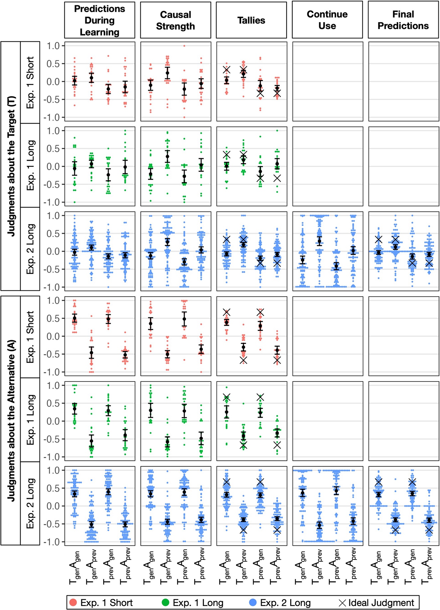
Figure 2 Raw individual judgments and means with 95% confidence intervals in Experiments 1 and 2.Note: Vertical jitter added for Causal Strength and Continue Use judgments. For Experiment 1, only data from Task 1 are presented.
2.3.1. Controlling
Controlling was assessed by comparing participants’ judgments about T in the Tgen conditions, which should be positive, with the Tprev conditions, which should be negative. In Figure 2, this would appear as a main effect of T when making judgments about T (top half of Figure 2). Controlling would appear as a high–high–low–low pattern from left to right.
In the short-timeframe condition, there was a main effect of controlling for all three dependent variables, ps < .01, BFs between 5.57 and 104 (left column in Table 3). This key finding replicates past studies that have found that people are able to control for alternative causes in traditional rapid trial-by-trial designs.
In the long timeframe, the evidence for controlling is much less clear. Only one p-value was significant (.046), and the strongest BF was 1.56.
With regard to the impact of timeframe, though the amount of controlling is numerically larger in the short timeframe when comparing the regression coefficients, the strongest p-value was .069 (BF = 1.14).
The regression weights for controlling for the Tally measure were compared with the ideal regression weight (.67). The regression weights were .28 in the short-timeframe condition and .13 in the long-timeframe condition, which means that they were only 42% and 20% as strong as they should be, respectively; both p’s < .001 and BFs > 108.
2.3.2. Simple learning
Simple learning was assessed by comparing participants’ judgments about A in the Agen conditions, which should be positive, with the Aprev conditions, which should be negative. In Figure 2, this would appear as a main effect of A when making judgments about A (bottom half of Figure 2). Simple learning would appear as a high–low–high–low pattern from left to right.
Across both the short and long timeframes, and across all three measures, the p-values and BFs all provided very strong support in favor of simple learning, ps < .001, BFs > 1011 (second column in Table 3). This finding is important as it is the first time that learning about two causes over a long timeframe has been assessed.
The tests for differences in simple learning in the short versus long timeframes produced only one marginal effect (p = .065, BF = .57), so there is minimal evidence of a difference in simple learning between the short and long conditions.
Despite there being clear evidence of simple learning in both timeframes, there was also evidence that learning was suboptimal. The Tally regression weights for simple learning were .68 for short and .62 for long. In comparison, the ideal regression weight is 1.33, which means that the regression weights were only 51% and 47% as strong as they should be, respectively, and they were significantly below 1.33; p’s < .001, BFs > 1019.
2.3.3. Discounting
Discounting was tested in two ways: whether A has a contrastive effect when judging T (Adiscounting), and whether T has a contrastive effect when judging A (Tdiscounting). Though both discounting effects are possible, the first one is more likely to occur as typically the stronger cause (A) has a discounting impact on the weaker (T).
Because discounting is not normative, this cannot be seen in the ideal judgments in the figures. In Figure 2, A Discounting shows up as a negative main effect of A on Judgments about T in the top half, and TDiscoutning shows up as a negative main effect of T on judgments about A in the bottom half of Figure 2. When there are strong Simple Learning and Controlling main effects, the Discounting effects can be hard to see in Figure 2.
For ADiscounting (the impact of A when judging T), there was clear evidence of discounting for the Causal Strength measure in both the short and long timeframes, ps ≤ .001, BFs > 27. There was some evidence for discounting on the Tally measure in the long timeframe but not the short, and the p-value for the Predictions during Learning was marginal in the long, but not the short. The comparisons between the short and long timeframes did not reveal any reliable differences.
For TDiscounting (the impact of T when judging A), there were two marginal p-values, but all of the BFs were less than 1, and most were in the range of .10–.15. In sum, there does not appear to be much if any discounting of the alternate by the weaker target.
There was no evidence of a difference between timeframes for either type of discounting.
2.4. Discussion
Experiment 1 found three key results and left some open questions. First, participants were able to learn simple cause–effect relations when they did not need to control, in both the short and long timeframes. Second, there was some evidence of discounting in both timeframes, particularly in the causal strength judgments for the target. Third, there was definitive evidence that participants controlled for the alternative in the short timeframe, but also that the amount of controlling was less than it should have been.
At the same time, the most important and novel test was whether participants could control for A when judging T in the long-timeframe condition. Unfortunately, there was no reliable evidence for this question according to the p-values and the BFs. It was clear that the degree of controlling was insufficient compared to the normative value, but it was not clear if controlling was significantly above zero in the long timeframe as the p-values were marginal and the BFs were weak. (Note that the within-subject analysis in Appendix B of the Supplementary Material found clearer evidence of controlling in the long timeframe, and the regression coefficients are similar to those in the between-subjects analysis, so the difference may just be due to power.) Furthermore, the comparison of the degree of controlling between the short and long conditions did not produce reliable evidence of a difference or a null effect. The lack of clear evidence of whether participants can control in the long timeframe motivated Experiment 2.
3. Experiment 2
3.1. Methods
There were two main differences between Experiments 1 and 2. First, because the most important question was whether people can control for alternative causes in more realistic long-timeframe situations, not whether there is a difference between long and short, and because there appeared to be some order effects when both tasks were tested, in Experiment 2, only the long-timeframe condition was used for increased power. Second, the sample size was increased for additional power. Third, two dependent measures were added to gain a more comprehensive understanding of how people make causal judgments when learning over long timeframes.
3.1.1. Participants
The goal was to recruit at least 400 participants so that there were 100 participants in each condition. This number was chosen by comparing BFs when the data from Experiment 1 were doubled, tripled, or quadrupled; a sample size of 400 was determined to be sufficient to produce strong BFs in support of either the null or alternative hypothesis. Participants had to be between the ages of 18 and 30 to achieve a similar sample to Experiment 1.
Anticipating that some participants would have to be excluded, 451 participants were recruited through advertisements on Facebook and advertisements were run in multiple east-coast cities. They were paid $20 if they completed the entire study. Participants were terminated from the study or excluded from analyses for the following reasons: missing 4 days (N = 11), not being in Eastern Standard Time for the duration of the study (N = 7), failing one of the attention checks described below (N = 30), or admitting to writing down notes about the data (N = 5). Thus, 398 were included in the final analyses.
Their mean age was 23.9 years (SD = 3.5), and the 5th and 95th percentiles were 19 and 30 years. With regard to sex, 78% identified as female, 16% as male, 6% as non-binary, and 6% did not report. With regard to ethnicity, 7% reported being Hispanic or Latino, 90% not, and 3% did not report. With regard to race, 1% identified as American Indian or Alaska Native, 26% as Asian, 7% as Black or African American, 1% as Native Hawaiian or Other Pacific Islander, 69% as White, and 2% did not report. Lastly, 33% were undergraduate students, 25% were graduate students, and 41% were not currently students.
3.1.2. Design
The same stimuli and datasets from Experiment 1 were used, but only with the long-timeframe condition. Thus, Experiment 2 was a 2 T (generative vs. preventative; between-subjects) × 2 A (generative vs. preventative; between-subjects) design.
3.1.3. Procedure
The procedure was very similar to Experiment 1, minus the short-timeframe condition. The entire study lasted 25 days. On Day 1, participants met with a research assistant via Zoom, completed an eight-trial practice task, and then did Day 1 of the long task. On Days 2–24, they completed the remaining trials for the long task. If participants missed 1 day (8%), 2 days (3%), or 3 days (1%) of the study, the subsequent trials were pushed back so that they experienced each trial on a different day. Most participants completed the dependent measures on Day 25 (97%), but some completed them either 2 days later (2%) and one completed them 4 days later.
Because the participants were recruited and run entirely online, three attention checks were added. During the sign-up process, participants had to pass Oppenheimer et al.’s (2009) sports measure. Two attention checks were added during the eight-trial practice task. At the beginning of the practice task, participants read an overview of the cover story and had to correctly recognize which medication names were used in the cover story; one participant did not pass this attention check. At the end of the practice task, participants recalled the number of times they observed each event type. Twenty-nine participants were not allowed to continue because they made judgments that added up to 16 or more trials.Footnote 8
3.1.4. Dependent measures
The predictions during learning measure was calculated over the last 14 trials (as opposed to the last 13 trials) so that participants saw at least one instance of each event type that was necessary for the calculations. In most cases, the average of Equations (2) and (3) were used for the tally measure strength and predictions during learning. For 1% of participants for the Tally measure and 13% of participants for the Predictions during Learning, only one of the two equations could be calculated. Two participants were dropped from analyses of Tallies for the assessment of T because neither equation was calculable.
Two other measures were included (see Zhang and Rottman, Reference Zhang and Rottman2023, for other uses of these measures). First, participants answered a question termed ‘continue use’: ‘Do you think you should continue to use [Medicine]?’. They made a continue-use judgment for both T and A, using a 21-point scale (−10 = definitely no, 0 = unsure, +10 = definitely yes), which was transformed onto a scale of −1 to +1. The reason for including this measure it is more oriented toward making a practical decision than the others. The causal strength and continue-use measures were asked after Trials 8, 16, and 24, similar to in Experiment 1.
Second, a measure termed ‘final prediction’ was asked on the last day of testing. This measure involved asking four questions and then transforming the questions into one judgment about T and one judgment about A. Participants were asked ‘Imagine that today (Day 25), you [take/do not take T] and [take/do not take A], what is the likelihood that you would experience [effect]?’. For each question, they could answer any number between 0 and 100. The average of Equations (2) and (3) was used to calculate final predictive strength. This measure was intended to be similar to the predictions during learning but to assess what has been learned by the end of the study.
3.2. Results and discussion
The inferential statistics are presented in Table 4, and the findings are visualized in Figure 2.
Table 4 Regression results for judgments in Experiment 2
3.2.1. Controlling
The larger sample for Experiment 2 produced definitive evidence that people can control for an alternative cause when learning about two causes over weeks. Across all measures, participants controlled for A when judging T, all ps < .001, all BFs > 100. The regression coefficients look similar, perhaps slightly stronger, than those in Experiment 1.
In Experiment 2, there were two measures—tallies and final predictive strength—that could be compared to an ideal judgment. Both were considerably weaker than optimal (b = 0.67, p’s < .001, BFs > 1042), implying that the ability to control for A is suboptimal.
3.2.2. Simple learning
Similar to Experiment 1, there was strong evidence for simple learning. And similar to Experiment 1, the learning was suboptimal; the regression weights were significantly weaker than the true weight (b = 1.33) for both tallies and final predictive strength, ps < .001, BFs > 1069.
3.2.3. Discounting
All of the measures of ADiscounting, with one exception, revealed that participants discounted when judging T; all ps ≤ .001, BFs > 31. The one exception was for the Predictions during Learning; p = .032, BF = 1.38. The predictions during learning was also the weakest measure in Experiment 1, and this will be discussed in Section 4. There was no evidence that participants discounted when judging A (the TDiscounting coefficient); all the BFs were in the direction of the null, and some were fairly strong in the direction of the null.
4. General discussion
This is the first study to test whether people can accurately learn about two confounded causes over many weeks. Controlling for alternative causes is closely related to the credit assignment problem in reinforcement learning, and controlling and discounting are closely related to many different phenomena involving cue competition in associative learning paradigms. Thus, the implications of these findings are pertinent to many findings beyond causal learning and reasoning. The key findings are broken down into three phenomena: controlling, simple learning, and discounting.
4.1. Controlling
The main goal of this research was to assess whether people could control for an alternative cause when engaged in causal learning and judgment over a long timeframe. When two causes are confounded, reaching an accurate causal conclusion requires controlling for the alternative confounded causes. Whereas Experiment 1 was somewhat inconclusive about whether participants controlled in the long timeframe, Experiment 2 provided very strong evidence that participants did control for the alternative cause in the long timeframe. Furthermore, the similarity in the regression coefficients for Experiments 1 and 2 suggests that the findings were very aligned and the differences were probably just a result of lower power in Experiment 1.
However, there is a major caveat to this point; the results show that the amount of controlling was quite small. Controlling was only about 20%–30% as strong as it should have been in the long timeframe and about 42% as strong as it should have been in the short timeframe. Whereas previous studies have primarily used causal strength judgments that cannot be compared to a normative value, the tallies and final predictive strength measures allow for a direct comparison between participants’ judgments to a normative standard. Therefore, whereas previous studies that have tested controlling in the short timeframe have concluded that people can control (relative to not at all), they omitted the fact that controlling is, in fact, fairly weak.
4.2. Simple learning
Strong evidence that people could learn about the ‘alternative’ cause, a simple cause–effect relation that does not require controlling, was found in both the short and long timeframes; this was termed ‘simple learning’. The alternative cause is fairly easy to learn about because it has roughly the same influence on the effect whether one controls for the target or not. Our finding that people can learn about the alternative in the long timeframe aligns with prior findings that people can learn causal relations between a single cause and effect about as well in the long as in the short timeframe (Willett and Rottman, Reference Willett and Rottman2021). The novel aspect of the current study is that people can also learn about simple causal relations when there are two causes in the long timeframe, not just one. At the same time, simple learning was only about 47%–55% as strong as it should have been in the long timeframe and 51% in the short timeframe.
4.3. Discounting
This research found very strong evidence of discounting, a non-normative pattern of reasoning, in both the short and long timeframes and across a variety of dependent measures. Most studies on controlling were not designed to test for discounting; it is only because the current studies used the complete 2 (alternative: generative or preventative) × 2 (target: generative or preventative) design that both controlling and discounting were able to be tested.
Prior research has suggested that discounting may have more to do with a decision process than a learning process. The idea is that when judging the strength of one cause people compare it to the strengths of other causes (Denniston et al., Reference Denniston, Savastano and Miller2001; Goedert and Spellman, Reference Goedert and Spellman2005; Laux et al., Reference Laux, Goedert and Markman2010; Miller and Matzel, Reference Miller and Matzel1988; Stout and Miller, Reference Stout and Miller2007). One hypothesis is that discounting may arise only at the time of making a judgment, when comparing cues, not during learning. This could result in discounting for the measures at the end of the study but not for the predictions during learning. In fact, the predictions during learning measure tended to produce nonsignificant or marginal discounting effects, weaker than other measures, which fits with this hypothesis. At the same time, the final predictive strength measure, which is similar though not exactly the same as the predictions during learning in Experiment 2, did find discounting. And the tally measure, though nonsignificant for the short timeframe in Experiment 1, was significant for discounting for the long timeframe in Experiments 1 and 2; it is not obvious why these memory questions would instigate a cue comparison process. Therefore, the current results provide mixed support for this hypothesis that discounting arises through a decision process rather than a learning process. They raise the possibility that participants’ memories may be distorted in the direction of discounting from the learning process or that their memories and some of their predictions may be based on their beliefs about causal strength.
4.4. Comparisons between short and long timeframes and other potential moderators of learning
The set of studies that my lab has recently been conducting on causal learning over a long timeframe has been designed to systematically examine whether various factors in how people experience events over time make it harder or easier to learn causal relations (Willett and Rottman, Reference Willett and Rottman2021; Zhang and Rottman, Reference Zhang and Rottman2023, Reference Zhang and Rottman2024). Some of these studies have looked at short versus long timeframes, and others have looked at different aspects of long-timeframe learning, such as the length of delay between a cause and effect.
Testing for differences between the short and long timeframe helps reveal the generalizability of existing short-timeframe findings to more real-world settings, and could provide useful data for developing theories about causal learning within and across the two settings. With this regard, an unfortunate outcome from Experiment 1 was that there was some uncertainty as to whether controlling and simple learning differed for the short versus long timeframes. There were no significant differences in controlling between the two timeframes; the Tallies measure revealed the strongest effect of timeframe, but the p-value was .069 and the BF was 1.14. In the within-subjects analysis in Appendix B of the Supplementary Material, this difference for Tallies was significant, p = .005, BF = 10.50, suggesting that perhaps there is a reliable difference in timeframes for the Tally measure with more power. In sum, although a longer timeframe may impair controlling, if there is an impairment, it is fairly modest, and only seen for one out of three measures.
For simple learning, none of the three measures revealed a reliable difference when only analyzing the first task. (As noted in Appendix B of the Supplementary Material, when both tasks were analyzed, there were reliable differences between timeframes; however, this appears to be driven by an order effect, and thus a cautious approach of focusing only on the first task seems most wise.)
Although it would have been nice to answer the question about differences between the short and long timeframes more definitively, the presence of order effects makes it very challenging to do so. It is not feasible to do a study in which participants are randomly assigned to a long-timeframe task versus a short-timeframe task as there would be challenges with regard to differences in incentives and dropout.
Rather than double down and rerun Experiment 1 with a much larger sample, I decided to focus on how accurately people learned in the long timeframe to obtain strong evidence of whether people could control at all in long-timeframe environments. The reason for this decision is that I view the long timeframe as the best simulation of real-world learning and therefore the most important topic to study. Experiment 2, with 398 participants, was able to obtain very strong evidence that people can control in the long timeframe while also providing evidence that the amount of controlling is quite modest.
Although the current findings hint at differences in learning between the short and long timeframes, they were not strong. However, ongoing research in my lab suggests that there are important differences. In particular, even though people are able to learn about cause–effect relations involving multiple potential causes and multiple potential effects in the short timeframe, we have found that learning appears to be much worse in the long timeframe (Zhang, Reference Zhang2025). There are a number of differences between the current study and the ones conducted by Zhang (Reference Zhang2025). First, in the current study, there were only two potential causal relations; Zhang (Reference Zhang2025) investigated situations with six and nine potential relations. Second, in the current study, the causes and effects occurred at the same time, whereas in Zhang (Reference Zhang2025), there were delays between the causes and effects. Third, in the current study, it was vital to control for the alternative cause when assessing the target, whereas in Zhang (Reference Zhang2025), the cause–effect relations were all quite strong and did not vary based on whether a third variable was or was not controlled for. Although Zhang (Reference Zhang2025) provides fairly clear evidence for a difference, the exact reasons for the increased difficulty in the long timeframe are not yet known.
In sum, there are many important further questions about how well people can learn causal relations that require controlling for alternative causes in real-world situations. The main conclusion from this research, that people can control for alternative causes when learning over a long timeframe, should not be generalized to all situations; there are very likely other moderators. At the same time, it is also hard to image factors in naturalistic situations that would make causal learning and judgment with two confounded causes much easier than in the current studies.
4.5. Comparisons to ideal judgments
Most of the measures in this research involved a participant making an inference; these were not compared to an ideal because there is not one true answer. Many alternative versions of rational or ideal standards have been put forth for how people make causal inferences (see Hattori and Oaksford, Reference Hattori and Oaksford2007, for a list). For example, ΔP is one way to assess the strength of a causal relation and involves assessing the difference in the probability of the effect when the causes are present versus absent. One downside of this measure is that the calculation of the strength of one cause is affected by the base rate of the effect. For example, suppose that the effect is present 90% of the time when the cause is absent; even if the cause always produces the effect, the ΔP value would only be .10. Another metric called PowerPC (Cheng, Reference Cheng1997) accounts for the base rate of the effect when the cause is absent; in the case mentioned in the prior sentence, the PowerPC value would be 1.00. Alternatively, other models of causal inference (e.g., Griffiths and Tenenbaum, Reference Griffiths and Tenenbaum2005; Lu et al., Reference Lu, Yuille, Liljeholm, Cheng and Holyoak2008) are sensitive to sample size, so they assess the confidence of the relation, similar to a p-value, rather than just the effect size of the relation. These models also involve priors on the plausible strengths of the effect, and the choice of prior can affect the strength of the inference as well as predictions about cue competition (Powell et al., Reference Powell, Merrick, Lu and Holyoak2016).
Because there are multiple options for normative standards, arguing that inferential judgments deviate from one particular standard is fraught. However, the tally measure can be directly compared to an ideal standard. The tally measure simply involved a series of questions about participants’ memories of the experienced events; it does not involve making an inference. Thus, it is hard to explain away why the memories would be distorted from a rational perspective. Furthermore, any potential explanation would have to account for both insufficient controlling and discounting. The final predictions in Experiment 2 were also compared to an ideal standard. In contrast to the tallies, the final predictions are more open to such critiques about alternative rational inferential processes. Predictions could be made by simply recalling the proportion of experienced events that led to one outcome versus the other. However, predictions could also be made by first making a causal inference and then making predictions from the inference.
In sum, I argue that the tally measure is an effective way to capture weaknesses in learning that are not sensitive to different possible normative standards or different possible priors. More broadly, though comparing the judgments to an ideal is one important contribution of this research, most of the analyses tested other hypotheses that are not sensitive to this critique.
4.6. Open questions
Aside from the open questions already discussed, there are three additional open questions. First, it is possible that with more than 24 trials, learning may approach ideal levels. When learning about a single cause, 24 trials were sufficient to produce approximately correct judgments (Willett and Rottman, Reference Willett and Rottman2021); however, perhaps more trials are needed with two causes. Indeed, in Spellman’s (Reference Spellman1996) study that served as the inspiration for this one, there were 80 trials; participants also provided judgments after 40 trials, but those judgments were not reported. In contrast, the current study only used 24 trials as we felt that it was not feasible to run a study for 40 days, let alone 80. So perhaps the difference in the number of trials could account for the different emphasis in the results that people control for alternative causes well versus not well. At the same time, insufficient learning was seen even in the tally measure; it is not obvious why the tally judgments would be affected by sample size even if other judgments are. Furthermore, from a practical perspective, 24 days is already a considerable length of time; people often make causal assessments from even less than 24 trials. For example, when starting a new medication, one may start to decide about the efficacy of the medicine considerably earlier than 24 days.
Second, as discussed in the Introduction, Derringer and Rottman (Reference Derringer and Rottman2018) found that when learning about multiple causes, people tend to utilize ‘informative transitions’, when one cause changes and the other remains the same, for causal inference. This theory served as one reason why learning might be considerably worse when spaced out over a long timeframe, as it could be hard to remember what happened the prior day, or the prior day may not be all that salient. However, the current studies do not permit a direct test of the Informative Transitions theory; future research should test whether this Informative Transitions learning process is used in long timeframes.
Third, comparing short- and long-timeframe learning raises a number of other potential processes and questions not explored here. The short-timeframe condition in Experiment 1, like many other short-timeframe studies, used a cover story that explains to participants that they will be presented with data that are sped up from how they would occur in real life. This raises a question of what happens when the learner’s experience of a causal mechanism is on a different order of magnitude from how they would ordinarily experience the mechanism and their expectations about the speed of the mechanism. A related question has to do if there is a discrepancy between the timing of a real-world process versus the one experienced in a psychology study, but participants know that the study is a sped-up simulation: Does this discrepancy matter? Expectations about the speed of mechanisms have a profound impact on causal inference (e.g., Buehner and McGregor, Reference Buehner and McGregor2006). Some research has also investigated the impact when learning is sped up even faster than is typical in short-timeframe learning (e.g., Allan et al., Reference Allan, Hannah, Crump and Siegel2008; Crump et al., Reference Crump, Hannah, Allan and Hord2007; Rehder et al., Reference Rehder, Davis and Bramley2022). Considering the range of presentations from extremely fast to very slow raises many questions about the roles of different cognitive systems, from perception and attention which are typically studied in fast presentations, to short-term memory, to long-term memory. On the one hand, the fact that there are similarities in learning across such radically different timescales that rely on different cognitive systems is remarkable. On the other hand, findings of differences, when learning occurs at different speeds (e.g., Rehder et al., Reference Rehder, Davis and Bramley2022), show the important role of human cognition in this learning process.
4.7. Conclusion
This study is the first to provide evidence that people engage in both normative and non-normative types of credit assignment when learning over long timeframes. Critically, these studies revealed evidence that people can learn simple cause–effect relations with multiple causes over a long timeframe and that people can control for alternative causes when learning over a long timeframe. However, both of these abilities were clearly suboptimal. Additionally, the strong non-normative discounting effect is concerning as it can lead to incorrect causal attributions.
Supplementary material
The supplementary material for this article can be found at http://doi.org/10.1017/jdm.2025.10006.
Data availability statement
See https://osf.io/3dajq/ for the analysis plan, data, and analysis code.
Acknowledgements
I thank Ciara Willett for her extensive contributions to all aspects of this project. This paper is dedicated in honor of Barbara Como, a research assistant, for her hard-working and inquisitive spirit, and her commitment to the lab. I also thank the research assistants who helped with data collection, including Barbara Como, Michael Datz, Isabella Demo, Julia Gillow, Watole Hamda, Beatrice Langer, Marissa LaSalle, Elizabeth Lawley, Brooke O’Hara, and Joanna Ye.
Funding statement
This work was supported by the National Science Foundation (Grant No. 1651330).
Competing interest
The author declares none.


 Open access