


1 Introduction
Given a smooth compact
 $d$
-manifold
$d$
-manifold
 ${\mathcal{M}}$
we are interested in the spectral properties of the Laplace–Beltrami operator
${\mathcal{M}}$
we are interested in the spectral properties of the Laplace–Beltrami operator
 $\unicode[STIX]{x1D6E5}$
on
$\unicode[STIX]{x1D6E5}$
on
 ${\mathcal{M}}$
. It is well known that the eigenvalue spectrum of
${\mathcal{M}}$
. It is well known that the eigenvalue spectrum of
 $\unicode[STIX]{x1D6E5}$
is purely discrete, i.e., the set of numbers
$\unicode[STIX]{x1D6E5}$
is purely discrete, i.e., the set of numbers
 $E$
admitting a solution to the Helmholtz equation
$E$
admitting a solution to the Helmholtz equation
 $$\begin{eqnarray}\unicode[STIX]{x1D6E5}\unicode[STIX]{x1D719}+E\unicode[STIX]{x1D719}=0\end{eqnarray}$$
is a sequence
 $\{{E_{\!j}\}}_{j\geqslant 1}$
of numbers ordered with multiplicity in a non-decreasing order such that
$\{{E_{\!j}\}}_{j\geqslant 1}$
of numbers ordered with multiplicity in a non-decreasing order such that
 $E_{j}\rightarrow \infty$
. We denote the corresponding sequence
$E_{j}\rightarrow \infty$
. We denote the corresponding sequence
 $\{{\unicode[STIX]{x1D719}_{j}\}}_{j\geqslant 1}$
of (real-valued) eigenfunctions constituting an orthonormal basis of the square-integrable functions
$\{{\unicode[STIX]{x1D719}_{j}\}}_{j\geqslant 1}$
of (real-valued) eigenfunctions constituting an orthonormal basis of the square-integrable functions
 $L^{2}({\mathcal{M}})$
on
$L^{2}({\mathcal{M}})$
on
 ${\mathcal{M}}$
; the sequence
${\mathcal{M}}$
; the sequence
 $\{{\unicode[STIX]{x1D719}_{j}\}}_{j\geqslant 1}$
is uniquely determined up to the spectral degeneracies (i.e., up to orthogonal transformations in each eigenspace of dimension
$\{{\unicode[STIX]{x1D719}_{j}\}}_{j\geqslant 1}$
is uniquely determined up to the spectral degeneracies (i.e., up to orthogonal transformations in each eigenspace of dimension
 ${\geqslant}2$
).
${\geqslant}2$
).
1.1 Shnirelman’s theorem and small-scale equidistribution
Assuming without loss of generality that
 ${\mathcal{M}}$
is unit volume
${\mathcal{M}}$
is unit volume
 $\operatorname{Vol}({\mathcal{M}})=1$
, the celebrated Shnirelman’s theorem [Reference Colin de Verdière9, Reference Shnirelman27, Reference Zelditch29] asserts that if
$\operatorname{Vol}({\mathcal{M}})=1$
, the celebrated Shnirelman’s theorem [Reference Colin de Verdière9, Reference Shnirelman27, Reference Zelditch29] asserts that if
 ${\mathcal{M}}$
is chaotic (i.e., the geodesic flow on
${\mathcal{M}}$
is chaotic (i.e., the geodesic flow on
 ${\mathcal{M}}$
is ergodic), then “most” of the
${\mathcal{M}}$
is ergodic), then “most” of the
 $\{\unicode[STIX]{x1D719}_{j}\}$
are
$\{\unicode[STIX]{x1D719}_{j}\}$
are
 $L^{2}$
-equidistributed. In particular, they are equidistributed in position space, i.e., there exists a density-
$L^{2}$
-equidistributed. In particular, they are equidistributed in position space, i.e., there exists a density-
 $1$
sequence
$1$
sequence
 $j_{k}$
such that for all “nice” domains
$j_{k}$
such that for all “nice” domains
 ${\mathcal{A}}\subseteq {\mathcal{M}}$
, we have
${\mathcal{A}}\subseteq {\mathcal{M}}$
, we have
 $$\begin{eqnarray}\displaystyle \lim _{k\rightarrow \infty }\int _{{\mathcal{A}}}\unicode[STIX]{x1D719}_{j_{k}}(x)^{2}\,dx=\operatorname{Vol}({\mathcal{A}}). & & \displaystyle\end{eqnarray}$$
Beyond Shnirelman’s theorem, Berry’s universality conjecture [Reference Berry3, Reference Berry4] implies that for a generic chaotic manifold (1.1) holds for
 ${\mathcal{A}}$
shrinking with
${\mathcal{A}}$
shrinking with
 $k$
slower than the Planck scale
$k$
slower than the Planck scale
 $E_{\!j_{k}}^{-1/2}$
. More precisely, it states that there exists a density-
$E_{\!j_{k}}^{-1/2}$
. More precisely, it states that there exists a density-
 $1$
sequence
$1$
sequence
 $\{{j_{k}\}}_{k}$
so that if
$\{{j_{k}\}}_{k}$
so that if
 $r_{0}(E):\mathbb{R}_{{>}0}\rightarrow \mathbb{R}_{{>}0}$
satisfies
$r_{0}(E):\mathbb{R}_{{>}0}\rightarrow \mathbb{R}_{{>}0}$
satisfies
 $r_{0}(E)\cdot E^{1/2}\rightarrow \infty$
diverging arbitrarily slowly, then, for
$r_{0}(E)\cdot E^{1/2}\rightarrow \infty$
diverging arbitrarily slowly, then, for
 $B_{x}(r)$
the radius-
$B_{x}(r)$
the radius-
 $r$
geodesic ball in
$r$
geodesic ball in
 ${\mathcal{M}}$
centred at
${\mathcal{M}}$
centred at
 $x$
, we have
$x$
, we have
 $$\begin{eqnarray}\displaystyle \biggl|\int _{B_{x}(r)}\unicode[STIX]{x1D719}_{j_{k}}(y)^{2}\,dy-\operatorname{Vol}(B_{x}(r))\biggr|=o_{k\rightarrow \infty }(r^{d}) & & \displaystyle\end{eqnarray}$$
uniformly for all
 $x\in {\mathcal{M}}$
and
$x\in {\mathcal{M}}$
and
 $r>r_{0}(E_{\!j_{k}})$
, i.e.,
$r>r_{0}(E_{\!j_{k}})$
, i.e.,
 $$\begin{eqnarray}\displaystyle \sup _{\substack{ x\in {\mathcal{M}} \\ r>r_{0}(E_{\!j_{k}\!})}}\biggl|\frac{\int _{B_{x}(r)}\unicode[STIX]{x1D719}_{j_{k}}(y)^{2}\,dy}{\operatorname{Vol}(B_{x}(r))}-1\biggr|\rightarrow 0. & & \displaystyle\end{eqnarray}$$
The following recent results are rigorous manifestations of the small-scale (“shrinking balls”) statement (1.3). Luo and Sarnak [Reference Luo and Sarnak24, Theorem 1.2] established the small-scale equidistribution for Laplace eigenfunctions on the modular surface (assuming in addition that they are Hecke eigenfunctions), where
 $r>E^{-\unicode[STIX]{x1D6FC}}$
with a small
$r>E^{-\unicode[STIX]{x1D6FC}}$
with a small
 $\unicode[STIX]{x1D6FC}>0$
, and Young [Reference Young28], conditionally on the generalized Riemann hypothesis, refined this estimate for
$\unicode[STIX]{x1D6FC}>0$
, and Young [Reference Young28], conditionally on the generalized Riemann hypothesis, refined this estimate for
 $r>E^{-1/6+o(1)}$
holding for all such eigenfunctions. Hezari and Rivière [Reference Hezari and Rivière19] and independently Han [Reference Han15] established the equidistribution for Laplace eigenfunctions on manifolds of negative curvature on logarithmic scale (i.e.,
$r>E^{-1/6+o(1)}$
holding for all such eigenfunctions. Hezari and Rivière [Reference Hezari and Rivière19] and independently Han [Reference Han15] established the equidistribution for Laplace eigenfunctions on manifolds of negative curvature on logarithmic scale (i.e.,
 $r>(\log E)^{-\unicode[STIX]{x1D6FC}}$
for some
$r>(\log E)^{-\unicode[STIX]{x1D6FC}}$
for some
 $\unicode[STIX]{x1D6FC}>0$
) and Han [Reference Han16] considered random Laplace eigenfunctions on “symmetric” manifolds of high spectral degeneracy; here the higher the spectral degeneracy the smaller the allowed scale is. More recently, Han and Tacy [Reference Han and Tacy17] proved the small-scale equidistribution for random Gaussian combinations of eigenfunctions on compact manifolds for
$\unicode[STIX]{x1D6FC}>0$
) and Han [Reference Han16] considered random Laplace eigenfunctions on “symmetric” manifolds of high spectral degeneracy; here the higher the spectral degeneracy the smaller the allowed scale is. More recently, Han and Tacy [Reference Han and Tacy17] proved the small-scale equidistribution for random Gaussian combinations of eigenfunctions on compact manifolds for
 $r>E^{-1/2+o(1)}$
and de Courcy-Ireland [Reference de Courcy-Ireland10] showed that, with high probability, the
$r>E^{-1/2+o(1)}$
and de Courcy-Ireland [Reference de Courcy-Ireland10] showed that, with high probability, the
 $L^{2}$
-mass of random Gaussian spherical harmonics is, up to a small error, equidistributed, slightly above the Planck scale.
$L^{2}$
-mass of random Gaussian spherical harmonics is, up to a small error, equidistributed, slightly above the Planck scale.
1.2 Toral Laplace eigenfunctions
For the
 $d$
-dimensional torus
$d$
-dimensional torus
 $\mathbb{T}^{d}=\mathbb{R}^{d}/\mathbb{Z}^{d}$
,
$\mathbb{T}^{d}=\mathbb{R}^{d}/\mathbb{Z}^{d}$
,
 $d\geqslant 2$
, there are high spectral degeneracies; in this case Lester and Rudnick [Reference Lester and Rudnick23, Theorem 1.1] proved that the small-scale equidistribution is satisfied by a generic Laplace eigenfunction (also considered by Hezari and Rivière [Reference Hezari and Rivière18]). More precisely, they showed that every orthonormal basis
$d\geqslant 2$
, there are high spectral degeneracies; in this case Lester and Rudnick [Reference Lester and Rudnick23, Theorem 1.1] proved that the small-scale equidistribution is satisfied by a generic Laplace eigenfunction (also considered by Hezari and Rivière [Reference Hezari and Rivière18]). More precisely, they showed that every orthonormal basis
 $\{\unicode[STIX]{x1D719}_{j}\}$
admits a density-1 subsequence
$\{\unicode[STIX]{x1D719}_{j}\}$
admits a density-1 subsequence
 $\{\unicode[STIX]{x1D719}_{j_{k}}\}$
of Laplace eigenfunctions obeying (1.3), with
$\{\unicode[STIX]{x1D719}_{j_{k}}\}$
of Laplace eigenfunctions obeying (1.3), with
 $r_{0}(E)=E^{-\unicode[STIX]{x1D6FC}(d)}$
, where
$r_{0}(E)=E^{-\unicode[STIX]{x1D6FC}(d)}$
, where
 $\unicode[STIX]{x1D6FC}(d)$
is given by
$\unicode[STIX]{x1D6FC}(d)$
is given by
 $$\begin{eqnarray}\displaystyle \unicode[STIX]{x1D6FC}(d)<\frac{1}{2(d-1)}, & & \displaystyle\end{eqnarray}$$
an (almost) optimal Planck-scale result for
 $d=2$
, yet somewhat weaker than Berry’s conjecture for
$d=2$
, yet somewhat weaker than Berry’s conjecture for
 $d>2$
.
$d>2$
.
One can express the real toral Laplace eigenfunctions explicitly as a sum of exponentials
 $$\begin{eqnarray}\displaystyle f_{n}(x)=\mathop{\sum }_{\unicode[STIX]{x1D706}\in {\mathcal{E}}_{n}}c_{\unicode[STIX]{x1D706}}e(\langle x,\unicode[STIX]{x1D706}\rangle )\quad (c_{-\unicode[STIX]{x1D706}}=\overline{c_{\unicode[STIX]{x1D706}}}) & & \displaystyle\end{eqnarray}$$
for
 $$\begin{eqnarray}\displaystyle n\in S_{d}:=\{n=a_{1}^{2}+\cdots +a_{d}^{2}:\,a_{1},\ldots ,a_{d}\in \mathbb{Z}\} & & \displaystyle\end{eqnarray}$$
expressible as a sum of
 $d$
integer squares, and the corresponding frequencies
$d$
integer squares, and the corresponding frequencies
 $\unicode[STIX]{x1D706}$
are the standard lattice points
$\unicode[STIX]{x1D706}$
are the standard lattice points
 $$\begin{eqnarray}\displaystyle {\mathcal{E}}_{n}={\mathcal{E}}_{d;n}=\{\unicode[STIX]{x1D706}\in \mathbb{Z}^{d}:\,\Vert \unicode[STIX]{x1D706}\Vert ^{2}=n\} & & \displaystyle\end{eqnarray}$$
lying on the
 $(d-1)$
-dimensional sphere (a circle for
$(d-1)$
-dimensional sphere (a circle for
 $d=2$
) of radius
$d=2$
) of radius
 $\sqrt{n}$
; in this case the energy is
$\sqrt{n}$
; in this case the energy is
 $E=E_{n}=4\unicode[STIX]{x1D70B}^{2}n$
. We will assume without loss of generality that
$E=E_{n}=4\unicode[STIX]{x1D70B}^{2}n$
. We will assume without loss of generality that
 $f_{n}$
is
$f_{n}$
is
 $L^{2}$
-normalized, equivalent to
$L^{2}$
-normalized, equivalent to
 $$\begin{eqnarray}\displaystyle \Vert f_{n}\Vert _{L^{2}(\mathbb{T}^{d})}^{2}=\mathop{\sum }_{\unicode[STIX]{x1D706}\in {\mathcal{E}}_{n}}|c_{\unicode[STIX]{x1D706}}|^{2}=1. & & \displaystyle\end{eqnarray}$$
For every
 $n\in S_{d}$
, denote
$n\in S_{d}$
, denote
 $$\begin{eqnarray}\displaystyle N=N_{d;n}=\#{\mathcal{E}}_{n}. & & \displaystyle\end{eqnarray}$$
When
 $d=2$
, by Landau’s theorem,
$d=2$
, by Landau’s theorem,
 $\{n\leqslant x:\,n\in S_{2}\}\sim K(x/\sqrt{\log x})$
, where
$\{n\leqslant x:\,n\in S_{2}\}\sim K(x/\sqrt{\log x})$
, where
 $K>0$
is the “Landau–Ramanujan constant”. On average
$K>0$
is the “Landau–Ramanujan constant”. On average
 $N=N_{2;n}$
is of order of magnitude
$N=N_{2;n}$
is of order of magnitude
 $\sqrt{\log n}$
; however, for a density-1 sequence in
$\sqrt{\log n}$
; however, for a density-1 sequence in
 $S_{2}$
we have
$S_{2}$
we have
 $N=(\log n)^{\log 2/2+o(1)}.$
In general, for
$N=(\log n)^{\log 2/2+o(1)}.$
In general, for
 $n\in S_{2}$
we have
$n\in S_{2}$
we have
 $$\begin{eqnarray}N=n^{o(1)}.\end{eqnarray}$$
For
 $d=3$
, Siegel’s theorem asserts that for
$d=3$
, Siegel’s theorem asserts that for
 $n\not \equiv 0,4,7\,(8)$
,
$n\not \equiv 0,4,7\,(8)$
,
 $$\begin{eqnarray}N=N_{3;n}=n^{1/2+o(1)};\end{eqnarray}$$
since
 $x\mapsto 2^{a}x$
is a bijection between the solutions to
$x\mapsto 2^{a}x$
is a bijection between the solutions to
 $x_{1}^{2}+x_{2}^{2}+x_{3}^{2}=n$
and
$x_{1}^{2}+x_{2}^{2}+x_{3}^{2}=n$
and
 $x_{1}^{2}+x_{2}^{2}+x_{3}^{2}=4^{a}n$
, we can always assume that
$x_{1}^{2}+x_{2}^{2}+x_{3}^{2}=4^{a}n$
, we can always assume that
 $n\not \equiv 0,4,7\,(8)$
with no loss of generality.
$n\not \equiv 0,4,7\,(8)$
with no loss of generality.
Granville and Wigman [Reference Granville and Wigman14, Theorem 1.2] refined the aforementioned estimate by Lester–Rudnick for
 $d=2$
. They proved that in this case, (1.3) is valid slightly above the Planck scale
$d=2$
. They proved that in this case, (1.3) is valid slightly above the Planck scale
 $r_{0}(E)=E^{-1/2+o(1)}$
for all eigenfunctions
$r_{0}(E)=E^{-1/2+o(1)}$
for all eigenfunctions
 $f_{n}$
as in (1.5), corresponding to numbers
$f_{n}$
as in (1.5), corresponding to numbers
 $n$
so that the lattice points
$n$
so that the lattice points
 ${\mathcal{E}}_{n}$
are well separated (“Bourgain–Rudnick sequences”), a condition satisfied [Reference Bourgain and Rudnick7, Lemma 5] by “generic” integers
${\mathcal{E}}_{n}$
are well separated (“Bourgain–Rudnick sequences”), a condition satisfied [Reference Bourgain and Rudnick7, Lemma 5] by “generic” integers
 $n\in S_{2}$
in a strong quantitative sense, subsequently refined in [Reference Granville and Wigman14, Theorem 1.4]; see §2.2.
$n\in S_{2}$
in a strong quantitative sense, subsequently refined in [Reference Granville and Wigman14, Theorem 1.4]; see §2.2.
1.3 Averaging mass with respect to ball centre
For both the two-dimensional and the higher-dimensional tori it is possible to construct exceptional examples of sequences of toral eigenfunctions where the equidistribution condition is not satisfied: for
 $d\geqslant 2$
thin sequences [Reference Lester and Rudnick23, Theorem 3.1]
$d\geqslant 2$
thin sequences [Reference Lester and Rudnick23, Theorem 3.1]
 $\{\unicode[STIX]{x1D719}_{j_{k}\!}\}$
of eigenfunctions violating condition (1.2) at the Planck scale
$\{\unicode[STIX]{x1D719}_{j_{k}\!}\}$
of eigenfunctions violating condition (1.2) at the Planck scale
 $r\cdot E_{\!j_{k}}^{1/2}\rightarrow \infty$
, around the origin
$r\cdot E_{\!j_{k}}^{1/2}\rightarrow \infty$
, around the origin
 $x=0$
, and even stronger, for
$x=0$
, and even stronger, for
 $d\geqslant 3$
[Reference Lester and Rudnick23, Theorem 4.1 (construction by J. Bourgain)] eigenfunctions violating (1.2) with
$d\geqslant 3$
[Reference Lester and Rudnick23, Theorem 4.1 (construction by J. Bourgain)] eigenfunctions violating (1.2) with
 $r\gg E^{-\unicode[STIX]{x1D6FC}(d)}$
, where
$r\gg E^{-\unicode[STIX]{x1D6FC}(d)}$
, where
 $\unicode[STIX]{x1D6FC}(d)>1/2(d-1)$
, again around the origin
$\unicode[STIX]{x1D6FC}(d)>1/2(d-1)$
, again around the origin
 $x=0$
. In these cases, rather than keeping the ball centre
$x=0$
. In these cases, rather than keeping the ball centre
 $x=0$
at the origin, one may vary
$x=0$
at the origin, one may vary
 $x$
and study whether the “typical” discrepancy on the left-hand side of (1.2) is small, even if the existence of
$x$
and study whether the “typical” discrepancy on the left-hand side of (1.2) is small, even if the existence of
 $x$
so that the left-hand side of (1.2) is not small is known, so that, in particular, (1.3) is not satisfied.
$x$
so that the left-hand side of (1.2) is not small is known, so that, in particular, (1.3) is not satisfied.
A natural way to vary
 $x$
is to think of
$x$
is to think of
 $x$
as random, drawn uniformly in
$x$
as random, drawn uniformly in
 $\mathbb{T}^{d}$
. We define the random variable
$\mathbb{T}^{d}$
. We define the random variable
 $$\begin{eqnarray}\displaystyle X_{\!f_{n},r}=X_{\!f_{n},r;x}:=\int _{B_{x}(r)}f_{n}(y)^{2}\,dy & & \displaystyle\end{eqnarray}$$
and are interested in the distribution of
 $X_{\!f_{n},r}$
where
$X_{\!f_{n},r}$
where
 $x$
is drawn randomly uniformly in
$x$
is drawn randomly uniformly in
 $\mathbb{T}^{d}$
. The relevant moments are: expectation
$\mathbb{T}^{d}$
. The relevant moments are: expectation
 $$\begin{eqnarray}\displaystyle \mathbb{E}[X_{\!f_{n},r}]=\int _{\mathbb{T}^{d}}X_{\!f_{n},r;x}\,dx, & & \displaystyle\end{eqnarray}$$
higher centred moments
 $$\begin{eqnarray}\displaystyle \mathbb{E}[(X_{\!f_{n},r}-\mathbb{E}[X_{\!f_{n},r}])^{k}]=\int _{\mathbb{T}^{d}}(X_{\!f_{n},r;x}-\mathbb{E}[X_{\!f_{n},r}])^{k}\,dx,\quad k\geqslant 2, & & \displaystyle\end{eqnarray}$$
and in particular the variance
 $$\begin{eqnarray}\displaystyle {\mathcal{V}}(X_{\!f_{n},r})=\mathbb{E}[(X_{\!f_{n},r}-\mathbb{E}[X_{\!f_{n},r}])^{2}]. & & \displaystyle\end{eqnarray}$$
This approach of averaging the
 $L^{2}$
-mass with respect to the ball centre (and keeping
$L^{2}$
-mass with respect to the ball centre (and keeping
 $f_{n}$
fixed) was pursued by Granville–Wigman [Reference Granville and Wigman14] in the two-dimensional case, again slightly above the Planck scale
$f_{n}$
fixed) was pursued by Granville–Wigman [Reference Granville and Wigman14] in the two-dimensional case, again slightly above the Planck scale
 $r>E^{-1/2+o(1)}$
. In this regime, by proving an upper bound for
$r>E^{-1/2+o(1)}$
. In this regime, by proving an upper bound for
 ${\mathcal{V}}(X_{\!f_{n},r})$
beyond
${\mathcal{V}}(X_{\!f_{n},r})$
beyond
 $(\mathbb{E}[X_{\!f_{n},r}])^{2}=O(r^{4})$
, valid for all
$(\mathbb{E}[X_{\!f_{n},r}])^{2}=O(r^{4})$
, valid for all
 $n\in S_{2}$
, under some flatness assumption on
$n\in S_{2}$
, under some flatness assumption on
 $f_{n}$
(cf. Definition 1.4 below), they established (1.2) for ‘‘typical” if not all
$f_{n}$
(cf. Definition 1.4 below), they established (1.2) for ‘‘typical” if not all
 $x\in \mathbb{T}^{2}$
. It would be desirable to find a regime where it is possible to analyse the precise asymptotic behaviour of the variance
$x\in \mathbb{T}^{2}$
. It would be desirable to find a regime where it is possible to analyse the precise asymptotic behaviour of the variance
 ${\mathcal{V}}(X_{\!f_{n},r})$
of
${\mathcal{V}}(X_{\!f_{n},r})$
of
 $X_{\!f_{n},r}$
and, if possible, determine the limit distribution law for
$X_{\!f_{n},r}$
and, if possible, determine the limit distribution law for
 $X_{\!f_{n},r}$
; our principal results below achieve both of these in the two-dimensional case and the former in the three-dimensional one (see Theorems 1.1 and 1.3). Such an approach of bounding the discrepancy variance while averaging over ball centres was recently used by Sarnak [Reference Sarnak25] for mass distribution of forms on symmetric spaces and Humphries [Reference Humphries20] for mass distribution of automorphic forms.
$X_{\!f_{n},r}$
; our principal results below achieve both of these in the two-dimensional case and the former in the three-dimensional one (see Theorems 1.1 and 1.3). Such an approach of bounding the discrepancy variance while averaging over ball centres was recently used by Sarnak [Reference Sarnak25] for mass distribution of forms on symmetric spaces and Humphries [Reference Humphries20] for mass distribution of automorphic forms.
1.4 Statement of the main results for
 $d=2,3$
: asymptotics for the variance, central limit theorem
$d=2,3$
: asymptotics for the variance, central limit theorem

Our principal results below are applicable to “flat” functions for
 $d=2,3$
, understood in suitable, more and less restrictive, senses. For example, “Bourgain’s eigenfunction” [Reference Bourgain6]
$d=2,3$
, understood in suitable, more and less restrictive, senses. For example, “Bourgain’s eigenfunction” [Reference Bourgain6]
 $$\begin{eqnarray}\displaystyle f_{n}(x)=\frac{1}{\sqrt{N}}\mathop{\sum }_{\unicode[STIX]{x1D706}\in {\mathcal{E}}_{n}}\unicode[STIX]{x1D700}_{\unicode[STIX]{x1D706}}e(\langle x,\unicode[STIX]{x1D706}\rangle ) & & \displaystyle\end{eqnarray}$$
with
 $\unicode[STIX]{x1D700}_{\unicode[STIX]{x1D706}}=\pm 1$
for every
$\unicode[STIX]{x1D700}_{\unicode[STIX]{x1D706}}=\pm 1$
for every
 $\unicode[STIX]{x1D706}\in {\mathcal{E}}_{n}$
, i.e., corresponding to
$\unicode[STIX]{x1D706}\in {\mathcal{E}}_{n}$
, i.e., corresponding to
 $|c_{\unicode[STIX]{x1D706}}|=N^{-1/2},$
satisfies any of the flatness conditions in the most restrictive sense. Denote
$|c_{\unicode[STIX]{x1D706}}|=N^{-1/2},$
satisfies any of the flatness conditions in the most restrictive sense. Denote
 ${\mathcal{B}}_{n}$
to be the class of Bourgain’s eigenfunctions.
${\mathcal{B}}_{n}$
to be the class of Bourgain’s eigenfunctions.
Our first principal result determines the precise asymptotic behaviour of the variance
 ${\mathcal{V}}(X_{\!f_{n},r})$
for the two-dimensional case and moreover asserts that the moments of the standardized random
${\mathcal{V}}(X_{\!f_{n},r})$
for the two-dimensional case and moreover asserts that the moments of the standardized random
 $L^{2}$
-mass of
$L^{2}$
-mass of
 $f_{n}$
are asymptotically Gaussian; we subsequently deduce a central limit theorem (see Corollary 1.2). For the sake of elegance of presentation, it is formulated for Bourgain’s eigenfunctions (1.14); below we formulate a more general result which holds for a larger class of flat eigenfunctions (see Theorem 2.5 in §2) and later a result where the averaging over the ball centre
$f_{n}$
are asymptotically Gaussian; we subsequently deduce a central limit theorem (see Corollary 1.2). For the sake of elegance of presentation, it is formulated for Bourgain’s eigenfunctions (1.14); below we formulate a more general result which holds for a larger class of flat eigenfunctions (see Theorem 2.5 in §2) and later a result where the averaging over the ball centre
 $x$
is itself restricted to shrinking balls (Theorem 8.3 in §8).
$x$
is itself restricted to shrinking balls (Theorem 8.3 in §8).
Theorem 1.1 (Gaussian moments,
$d=2$
, Bourgain’s eigenfunctions).

There exists a density-1 sequence
 $S_{2}^{\prime }\subseteq S_{2}$
so that the following holds. Let
$S_{2}^{\prime }\subseteq S_{2}$
so that the following holds. Let
 $r_{0}=r_{0}(n)=n^{-1/2}T_{0}(n)$
with
$r_{0}=r_{0}(n)=n^{-1/2}T_{0}(n)$
with
 $T_{0}(n)\rightarrow \infty$
.
$T_{0}(n)\rightarrow \infty$
.
(1) Fix a number
$\unicode[STIX]{x1D716}>0$
and suppose that
$T_{0}(n)<(\log n)^{(1/2)\log (\unicode[STIX]{x1D70B}/2)-\unicode[STIX]{x1D716}}$
. Then as
$n\rightarrow \infty$
along
$S_{2}^{\prime }$
we have (1.15)uniformly for all$$\begin{eqnarray}\displaystyle {\mathcal{V}}(X_{\!f_{n},r})\sim \frac{16}{3\unicode[STIX]{x1D70B}}r^{4}T^{-1} & & \displaystyle\end{eqnarray}$$
(1.16)and$$\begin{eqnarray}\displaystyle r_{0}<r<n^{-1/2}(\log n)^{(1/2)\log (\unicode[STIX]{x1D70B}/2)-\unicode[STIX]{x1D716}} & & \displaystyle\end{eqnarray}$$
$f_{n}\in {\mathcal{B}}_{n}$
, where
$T:=n^{1/2}r$
.(2) Under the above notation, let
(1.17)be the standardized random$$\begin{eqnarray}\displaystyle \hat{X}_{\!f_{n},r}:=\frac{X_{\!f_{n},r}-\mathbb{E}[X_{\!f_{n},r}]}{\sqrt{{\mathcal{V}}(X_{\!f_{n},r})}} & & \displaystyle\end{eqnarray}$$
$L^{2}$
-mass of
$f_{n}$
,
$r_{1}=r_{1}(n)=n^{-1/2}T_{1}(n)$
and suppose further that the sequence of numbers
$T_{1}(n)>T_{0}(n)$
satisfies
$T_{1}(n)=O(N^{\unicode[STIX]{x1D709}})$
for every
$\unicode[STIX]{x1D709}>0$
. Then for all
$k\geqslant 3$
the
$k$
th moment of
$\hat{X}_{\!f_{n},r}$
converges, for
$n\rightarrow \infty$
along
$S_{2}^{\prime }$
, to the standard Gaussian moment (1.18)uniformly for$$\begin{eqnarray}\displaystyle \mathbb{E}[\hat{X}_{\!f_{n},r}^{k}]\rightarrow \mathbb{E}[Z^{k}] & & \displaystyle\end{eqnarray}$$
$r_{0}<r<r_{1}$
and
$f_{n}\in {\mathcal{B}}_{n}$
, where
$Z\sim N(0,1)$
is the standard Gaussian variable.


The claimed uniform asymptotics (1.15) of the variance means explicitly that, as
 $n\rightarrow \infty$
along
$n\rightarrow \infty$
along
 $S_{2}^{\prime }$
, one has
$S_{2}^{\prime }$
, one has
 $$\begin{eqnarray}\displaystyle \sup _{\substack{ r_{0}<r<(\log n)^{(1/2)\log (\unicode[STIX]{x1D70B}/2)-\unicode[STIX]{x1D716}} \\ f_{n}\in {\mathcal{B}}_{n}}}\biggl|\frac{{\mathcal{V}}(X_{\!f_{n},r})}{(16/3\unicode[STIX]{x1D70B})r^{4}T^{-1}}-1\biggr|\rightarrow 0 & & \displaystyle\end{eqnarray}$$
and the uniform convergence (1.18) of the moments means that for every
 $k\geqslant 3$
,
$k\geqslant 3$
,
 $$\begin{eqnarray}\sup _{\substack{ r_{0}<r<r_{1} \\ f_{n}\in {\mathcal{B}}_{n}}}|\mathbb{E}[\hat{X}_{f_{n},r}^{k}]-\mathbb{E}[Z^{k}]|\rightarrow 0.\end{eqnarray}$$
Concerning the restricted range (1.16) in Theorem 1.1 (and (1.19)) for the possible radii, it is directly related to a well-known result on the angular distribution of lattice points in
 ${\mathcal{E}}_{n}$
for generic
${\mathcal{E}}_{n}$
for generic
 $n\in S_{2}$
. Namely, it was shown [Reference Erdős and Hall11] that
$n\in S_{2}$
. Namely, it was shown [Reference Erdős and Hall11] that
 ${\mathcal{E}}_{n}$
, projected by homothety to the unit circle, is equidistributed and, moreover, a quantitative measure for the discrepancy is asserted (see §2.1 below and, in particular, (2.2)), satisfied by generic
${\mathcal{E}}_{n}$
, projected by homothety to the unit circle, is equidistributed and, moreover, a quantitative measure for the discrepancy is asserted (see §2.1 below and, in particular, (2.2)), satisfied by generic
 $n\in S_{2}$
. Bourgain [Reference Bourgain6] observed that
$n\in S_{2}$
. Bourgain [Reference Bourgain6] observed that
 $f_{n}\in {\mathcal{B}}_{n}$
, when averaged over
$f_{n}\in {\mathcal{B}}_{n}$
, when averaged over
 $x\in \mathbb{T}^{d}$
, exhibits Gaussianity in the following sense. Let
$x\in \mathbb{T}^{d}$
, exhibits Gaussianity in the following sense. Let
 $T>0$
be a fixed number and define the scaled function
$T>0$
be a fixed number and define the scaled function
 $\unicode[STIX]{x1D711}_{x}:[-1,1]^{2}\rightarrow \mathbb{R}$
around
$\unicode[STIX]{x1D711}_{x}:[-1,1]^{2}\rightarrow \mathbb{R}$
around
 $x$
as
$x$
as
 $$\begin{eqnarray}\displaystyle \unicode[STIX]{x1D711}_{x}(y):=f_{n}\bigg(x+\frac{T}{\sqrt{n}}\cdot y\bigg), & & \displaystyle\end{eqnarray}$$
i.e., the trace of
 $f_{n}$
on the side-
$f_{n}$
on the side-
 $2(T/\sqrt{n})$
square centred at
$2(T/\sqrt{n})$
square centred at
 $x$
. It was found [Reference Bourgain6] that, upon thinking of
$x$
. It was found [Reference Bourgain6] that, upon thinking of
 $x\in \mathbb{T}^{2}$
as random, and
$x\in \mathbb{T}^{2}$
as random, and
 $\unicode[STIX]{x1D711}_{x}(\cdot )$
as a random field indexed by
$\unicode[STIX]{x1D711}_{x}(\cdot )$
as a random field indexed by
 $[-1,1]^{2}$
, it converges, in a suitable sense, to a particular Gaussian field (“monochromatic isotropic waves”) on
$[-1,1]^{2}$
, it converges, in a suitable sense, to a particular Gaussian field (“monochromatic isotropic waves”) on
 $\mathbb{R}^{2}$
, restricted to
$\mathbb{R}^{2}$
, restricted to
 $[-1,1]^{2}$
. This allows one to infer some results on the (deterministic) functions
$[-1,1]^{2}$
. This allows one to infer some results on the (deterministic) functions
 $f_{n}\in {\mathcal{B}}_{n}$
from the analogous results on the limit Gaussian random field. We may then re-interpret the quantitative version (2.2) of the angular equidistribution of lattice points as allowing the parameter
$f_{n}\in {\mathcal{B}}_{n}$
from the analogous results on the limit Gaussian random field. We may then re-interpret the quantitative version (2.2) of the angular equidistribution of lattice points as allowing the parameter
 $T$
in (1.20) to grow as a (positive) logarithmic power of
$T$
in (1.20) to grow as a (positive) logarithmic power of
 $n$
, while still retaining the said asymptotic Gaussianity, also allowing for the comparison between the mass distribution of
$n$
, while still retaining the said asymptotic Gaussianity, also allowing for the comparison between the mass distribution of
 $f_{n}$
with respect to the position and mass distribution of monochromatic isotropic waves. Our intuition regarding the possibility of carrying on the explained “de-randomization” argument for establishing results of similar nature to the presented results was recently validated by Sartori [Reference Sartori26].
$f_{n}$
with respect to the position and mass distribution of monochromatic isotropic waves. Our intuition regarding the possibility of carrying on the explained “de-randomization” argument for establishing results of similar nature to the presented results was recently validated by Sartori [Reference Sartori26].
An application of the standard theory [Reference Feller12, §XVI.3, Lemma 2] allows us to infer a uniform central limit theorem for the random variables
 $\hat{X}_{\!f_{n},r}$
from the convergence (1.18) of their respective moments to the Gaussian ones.
$\hat{X}_{\!f_{n},r}$
from the convergence (1.18) of their respective moments to the Gaussian ones.
Corollary 1.2. In the setting of Theorem 1.1, part (2), the distribution of the random variables
 $\{\hat{X}_{\!f_{n},r}\}$
converges uniformly to the standard Gaussian distribution: as
$\{\hat{X}_{\!f_{n},r}\}$
converges uniformly to the standard Gaussian distribution: as
 $n\rightarrow \infty$
along
$n\rightarrow \infty$
along
 $S_{2}^{\prime }$
,
$S_{2}^{\prime }$
,
 $$\begin{eqnarray}\operatorname{meas}\{x\in \mathbb{T}^{2}:\,\hat{X}_{\!f_{n},r;x}\leqslant t\}\rightarrow \frac{1}{\sqrt{2\unicode[STIX]{x1D70B}}}\int _{-\infty }^{t}\text{e}^{-z^{2}/2}\,dz\end{eqnarray}$$
uniformly for
 $t\in \mathbb{R}$
,
$t\in \mathbb{R}$
,
 $r_{0}<r<r_{1}$
and
$r_{0}<r<r_{1}$
and
 $f_{n}\in {\mathcal{B}}_{n}$
.
$f_{n}\in {\mathcal{B}}_{n}$
.
For the three-dimensional case, for Bourgain’s eigenfunctions, we only claim a precise asymptotic result on
 ${\mathcal{V}}(X_{\!f_{n},r})$
, the good news being that the claimed result is valid for all energies satisfying the natural congruence assumptions.
${\mathcal{V}}(X_{\!f_{n},r})$
, the good news being that the claimed result is valid for all energies satisfying the natural congruence assumptions.
Theorem 1.3 (Asymptotics for the variance for
$d=3$
, Bourgain’s eigenfunctions).

There exists a number
 $\unicode[STIX]{x1D702}>0$
such that if
$\unicode[STIX]{x1D702}>0$
such that if
 $r_{0}=r_{0}(n)=n^{-1/2}T_{0}(n)$
with
$r_{0}=r_{0}(n)=n^{-1/2}T_{0}(n)$
with
 $T_{0}(n)\rightarrow \infty$
, then for all
$T_{0}(n)\rightarrow \infty$
, then for all
 $n\not \equiv 0,4,7\,(8)$
we have
$n\not \equiv 0,4,7\,(8)$
we have
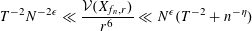
 $$\begin{eqnarray}{\mathcal{V}}(X_{\!f_{n},r})\sim r^{6}T^{-2}\end{eqnarray}$$
uniformly for
 $r_{0}<r<n^{-1/2+\unicode[STIX]{x1D702}}$
and
$r_{0}<r<n^{-1/2+\unicode[STIX]{x1D702}}$
and
 $f_{n}\in {\mathcal{B}}_{n}$
.
$f_{n}\in {\mathcal{B}}_{n}$
.
The meaning of the uniform statement in Theorem 1.3 is that
 $$\begin{eqnarray}\displaystyle \sup _{\substack{ r_{0}<r<n^{-1/2+\unicode[STIX]{x1D702}} \\ f_{n}\in {\mathcal{B}}_{n}}}\biggl|\frac{{\mathcal{V}}(X_{\!f_{n},r})}{r^{6}T^{-2}}-1\biggr|\rightarrow 0 & & \displaystyle\end{eqnarray}$$
as
 $n\rightarrow \infty$
along
$n\rightarrow \infty$
along
 $n\not \equiv 0,4,7\,(8)$
; cf. (1.19) in the two-dimensional case.
$n\not \equiv 0,4,7\,(8)$
; cf. (1.19) in the two-dimensional case.
1.5 Statement of the main results for
$d=2,3$
: more general upper and lower bounds

Let
 $f_{n}$
be as in (1.5) and consider the vector
$f_{n}$
be as in (1.5) and consider the vector
 $$\begin{eqnarray}\displaystyle \text{}\underline{v}:=(|c_{\unicode[STIX]{x1D706}}|^{2})_{\unicode[STIX]{x1D706}\in {\mathcal{E}}_{n}}\in \mathbb{R}^{{\mathcal{E}}_{n}} & & \displaystyle\end{eqnarray}$$
of the squared absolute values of its coefficients; we denote its normalized
 $\ell _{\infty }$
-norm by
$\ell _{\infty }$
-norm by
 $$\begin{eqnarray}\displaystyle [\text{}\underline{v}]_{\infty }:=N\cdot \max _{\unicode[STIX]{x1D706}\in {\mathcal{E}}_{n}}|c_{\unicode[STIX]{x1D706}}|^{2}. & & \displaystyle\end{eqnarray}$$
Definition 1.4 (Ultra-flat functions [Reference Granville and Wigman14, Definition 1.9]).
We say that an eigenfunction
 $f_{n}$
in (1.5) is
$f_{n}$
in (1.5) is
 $\unicode[STIX]{x1D716}$
-ultra-flat if its coefficients satisfy
$\unicode[STIX]{x1D716}$
-ultra-flat if its coefficients satisfy
 $$\begin{eqnarray}\displaystyle [\text{}\underline{v}]_{\infty }\leqslant N^{\unicode[STIX]{x1D716}}. & & \displaystyle\end{eqnarray}$$
Denote
 ${\mathcal{U}}_{n;\unicode[STIX]{x1D716}}$
to be the class of
${\mathcal{U}}_{n;\unicode[STIX]{x1D716}}$
to be the class of
 $\unicode[STIX]{x1D716}$
-ultra-flat functions.
$\unicode[STIX]{x1D716}$
-ultra-flat functions.
The following couple of theorems establish more general upper and lower bounds on
 ${\mathcal{V}}(X_{\!f_{n},r})$
in the two- and three-dimensional cases, respectively.
${\mathcal{V}}(X_{\!f_{n},r})$
in the two- and three-dimensional cases, respectively.
Theorem 1.5 (Bounds for the variance for ultra-flat eigenfunctions,
$d=2$
).

There exist a density-1 sequence
 $S_{2}^{\prime }\subseteq S_{2}$
and an absolute constant
$S_{2}^{\prime }\subseteq S_{2}$
and an absolute constant
 $C>0$
such that for every
$C>0$
such that for every
 $\unicode[STIX]{x1D716}>0$
,
$\unicode[STIX]{x1D716}>0$
,
 $\unicode[STIX]{x1D702}>0$
,
$\unicode[STIX]{x1D702}>0$
,
 $r_{0}=r_{0}(n)=n^{-1/2}T_{0}(n)$
with
$r_{0}=r_{0}(n)=n^{-1/2}T_{0}(n)$
with
 $T_{0}(n)\rightarrow \infty$
arbitrarily slowly and
$T_{0}(n)\rightarrow \infty$
arbitrarily slowly and
 $r=n^{-1/2}T>r_{0}$
, as
$r=n^{-1/2}T>r_{0}$
, as
 $n\rightarrow \infty$
along
$n\rightarrow \infty$
along
 $S_{2}^{\prime }$
, we have
$S_{2}^{\prime }$
, we have
 $$\begin{eqnarray}\displaystyle T^{-1}N^{-2\unicode[STIX]{x1D716}}\ll \frac{{\mathcal{V}}(X_{\!f_{n},r})}{r^{4}}\ll N^{\unicode[STIX]{x1D716}}\cdot (T^{-1}+(\log n)^{-(1/2)\log (\unicode[STIX]{x1D70B}/2)+\unicode[STIX]{x1D702}}) & & \displaystyle\end{eqnarray}$$
uniformly for
 $r_{0}<r<Cn^{-1/2}N^{1-\unicode[STIX]{x1D716}}$
and
$r_{0}<r<Cn^{-1/2}N^{1-\unicode[STIX]{x1D716}}$
and
 $f_{n}\in {\mathcal{U}}_{n;\unicode[STIX]{x1D716}}$
, where the constant involved in the “
$f_{n}\in {\mathcal{U}}_{n;\unicode[STIX]{x1D716}}$
, where the constant involved in the “
 $\ll$
”-notation in (1.25) is absolute for the lower bound and depends only on
$\ll$
”-notation in (1.25) is absolute for the lower bound and depends only on
 $\unicode[STIX]{x1D702}$
for the upper bound. Moreover, the upper bound is valid for the extended range
$\unicode[STIX]{x1D702}$
for the upper bound. Moreover, the upper bound is valid for the extended range
 $r>r_{0}$
(with no upper bound on
$r>r_{0}$
(with no upper bound on
 $r$
imposed) and the lower bound is valid for every
$r$
imposed) and the lower bound is valid for every
 $n\in S_{2}$
.
$n\in S_{2}$
.
Theorem 1.6 (Bounds for the variance for ultra-flat eigenfunctions,
$d=3$
).

There exist a number
 $\unicode[STIX]{x1D702}>0$
and a constant
$\unicode[STIX]{x1D702}>0$
and a constant
 $C>0$
such that for every
$C>0$
such that for every
 $\unicode[STIX]{x1D716}>0$
,
$\unicode[STIX]{x1D716}>0$
,
 $r_{0}=r_{0}(n)=n^{-1/2}T_{0}(n)$
with
$r_{0}=r_{0}(n)=n^{-1/2}T_{0}(n)$
with
 $T_{0}(n)\rightarrow \infty$
arbitrarily slowly,
$T_{0}(n)\rightarrow \infty$
arbitrarily slowly,
 $r=n^{-1/2}T>r_{0}$
and
$r=n^{-1/2}T>r_{0}$
and
 $n\not \equiv 0,4,7\,(8)$
, we have
$n\not \equiv 0,4,7\,(8)$
, we have
 $$\begin{eqnarray}\displaystyle T^{-2}N^{-2\unicode[STIX]{x1D716}}\ll \frac{{\mathcal{V}}(X_{\!f_{n},r})}{r^{6}}\ll N^{\unicode[STIX]{x1D716}}(T^{-2}+n^{-\unicode[STIX]{x1D702}}) & & \displaystyle\end{eqnarray}$$
uniformly for
 $r_{0}<r<Cn^{-1/2}N^{1-\unicode[STIX]{x1D716}}$
and
$r_{0}<r<Cn^{-1/2}N^{1-\unicode[STIX]{x1D716}}$
and
 $f_{n}\in {\mathcal{U}}_{n;\unicode[STIX]{x1D716}}$
, where the constants involved in the “
$f_{n}\in {\mathcal{U}}_{n;\unicode[STIX]{x1D716}}$
, where the constants involved in the “
 $\ll$
”-notation are absolute. Moreover, the upper bound in (1.26) is valid for the extended range
$\ll$
”-notation are absolute. Moreover, the upper bound in (1.26) is valid for the extended range
 $r>r_{0}$
.
$r>r_{0}$
.
For Bourgain’s eigenfunctions, the proofs of Theorems 1.5 and 1.6 yield slightly stronger bounds compared to (1.25) and (1.26), namely
 $$\begin{eqnarray}T^{-1}\ll \frac{{\mathcal{V}}(X_{\!f_{n},r})}{r^{4}}\ll T^{-1}+(\log n)^{-(1/2)\log (\unicode[STIX]{x1D70B}/2)+\unicode[STIX]{x1D716}}\end{eqnarray}$$
for
 $d=2$
and
$d=2$
and
 $$\begin{eqnarray}T^{-2}\ll \frac{{\mathcal{V}}(X_{\!f_{n},r})}{r^{6}}\ll T^{-2}+n^{-\unicode[STIX]{x1D702}}\end{eqnarray}$$
for
 $d=3$
.
$d=3$
.
1.6 Outline of the paper
The rest of the paper is organized as follows. In §2 we formulate Theorem 2.5, which, on one hand, generalizes Theorem 1.1 for a larger class of flat eigenfunctions and, on the other hand, explicates a sufficient condition on
 $n\in S_{2}$
for its statements to hold; a few examples of application of Theorem 2.5, corresponding to different asymptotic behaviours of the variance (2.14), are also discussed. Section 4 is dedicated to giving a proof of the first part of Theorem 1.1 (respectively the first part of Theorem 2.5), whereas the second part of Theorem 1.1 (respectively the second part of Theorem 2.5) is proved in §5. Theorem 1.3, claiming the precise asymptotics for the
$n\in S_{2}$
for its statements to hold; a few examples of application of Theorem 2.5, corresponding to different asymptotic behaviours of the variance (2.14), are also discussed. Section 4 is dedicated to giving a proof of the first part of Theorem 1.1 (respectively the first part of Theorem 2.5), whereas the second part of Theorem 1.1 (respectively the second part of Theorem 2.5) is proved in §5. Theorem 1.3, claiming the precise asymptotics for the
 $L^{2}$
-mass variance for Bourgain’s eigenfunctions in three dimensions, is proved in §6.
$L^{2}$
-mass variance for Bourgain’s eigenfunctions in three dimensions, is proved in §6.
In §7 we prove the various upper and lower bounds asserted by Theorems 1.5 and 1.6. A refinement of Theorem 2.5, where rather than draw
 $x$
with respect to the uniform measure on the full torus,
$x$
with respect to the uniform measure on the full torus,
 $x$
is drawn on balls slightly above the Planck scale, is presented in §8 and the additional subtleties of its proof as compared to the proof of Theorem 2.5 are highlighted. Finally, §9 contains the proofs of all auxiliary lemmas, postponed in course of the proofs of the various results.
$x$
is drawn on balls slightly above the Planck scale, is presented in §8 and the additional subtleties of its proof as compared to the proof of Theorem 2.5 are highlighted. Finally, §9 contains the proofs of all auxiliary lemmas, postponed in course of the proofs of the various results.
2 On Theorem 1.1: central limit theorem for mass distribution,
$d=2$

In this section we focus on Theorem 1.1. Our first goal is to formulate a result that, on one hand, generalizes the statement of Theorem 1.1 to a larger class of eigenfunctions and, on the other hand, provides a more explicit control over the generic numbers
 $n\in S_{2}$
. To this end we discuss the angular distribution of
$n\in S_{2}$
. To this end we discuss the angular distribution of
 $\unicode[STIX]{x1D706}\in {\mathcal{E}}_{n}$
(§2.1) and the spectral correlations (§2.2), also used in the course of the proof of the three-dimensional Theorem 1.3; we will be able to formulate Theorem 2.5, as prescribed above, by appealing to these. In §2.4 we consider a few scenarios when Theorem 2.5 is applicable, prescribing different asymptotic behaviours for the variance (2.14).
$\unicode[STIX]{x1D706}\in {\mathcal{E}}_{n}$
(§2.1) and the spectral correlations (§2.2), also used in the course of the proof of the three-dimensional Theorem 1.3; we will be able to formulate Theorem 2.5, as prescribed above, by appealing to these. In §2.4 we consider a few scenarios when Theorem 2.5 is applicable, prescribing different asymptotic behaviours for the variance (2.14).
2.1 Angular equidistribution of lattice points
For every
 $\unicode[STIX]{x1D706}=(\unicode[STIX]{x1D706}_{1},\unicode[STIX]{x1D706}_{2})\in {\mathcal{E}}_{n}$
, write
$\unicode[STIX]{x1D706}=(\unicode[STIX]{x1D706}_{1},\unicode[STIX]{x1D706}_{2})\in {\mathcal{E}}_{n}$
, write
 $\unicode[STIX]{x1D706}_{1}+i\unicode[STIX]{x1D706}_{2}=\sqrt{n}\text{e}^{i\unicode[STIX]{x1D719}}$
and denote the various angles by
$\unicode[STIX]{x1D706}_{1}+i\unicode[STIX]{x1D706}_{2}=\sqrt{n}\text{e}^{i\unicode[STIX]{x1D719}}$
and denote the various angles by
 $$\begin{eqnarray}0\leqslant \unicode[STIX]{x1D719}_{1}<\unicode[STIX]{x1D719}_{2}<\cdots <\unicode[STIX]{x1D719}_{N}<2\unicode[STIX]{x1D70B}.\end{eqnarray}$$
Recall that the discrepancy of the sequence
 $\unicode[STIX]{x1D719}_{j}$
is defined by
$\unicode[STIX]{x1D719}_{j}$
is defined by
 $$\begin{eqnarray}\displaystyle \unicode[STIX]{x1D6E5}(n)=\sup _{0\leqslant a\leqslant b\leqslant 2\unicode[STIX]{x1D70B}}\biggl|\frac{1}{N}\cdot \#\{1\leqslant j\leqslant N:\,\unicode[STIX]{x1D719}_{j}\in [a,b]\,\text{mod}\,2\unicode[STIX]{x1D70B}\}-\frac{(b-a)}{2\unicode[STIX]{x1D70B}}\biggr|. & & \displaystyle \nonumber\\ \displaystyle & & \displaystyle\end{eqnarray}$$
For every
 $\unicode[STIX]{x1D716}>0$
, we say that
$\unicode[STIX]{x1D716}>0$
, we say that
 $n\in S_{2}$
satisfies the hypothesis
$n\in S_{2}$
satisfies the hypothesis
 ${\mathcal{D}}(n,\unicode[STIX]{x1D716})$
if
${\mathcal{D}}(n,\unicode[STIX]{x1D716})$
if
 $$\begin{eqnarray}\displaystyle \unicode[STIX]{x1D6E5}(n)\leqslant (\log n)^{-(1/2)\log (\unicode[STIX]{x1D70B}/2)+\unicode[STIX]{x1D716}}. & & \displaystyle\end{eqnarray}$$
By Erdős–Hall [Reference Erdős and Hall11, Theorem 1], there exists a density-1 sequence
 $S_{2}^{\prime }(\unicode[STIX]{x1D716})\subseteq S_{2}$
such that
$S_{2}^{\prime }(\unicode[STIX]{x1D716})\subseteq S_{2}$
such that
 ${\mathcal{D}}(n,\unicode[STIX]{x1D716})$
is satisfied for every
${\mathcal{D}}(n,\unicode[STIX]{x1D716})$
is satisfied for every
 $n\in S_{2}^{\prime }(\unicode[STIX]{x1D716})$
. By a standard diagonalization argument, there exists a density-1 sequence
$n\in S_{2}^{\prime }(\unicode[STIX]{x1D716})$
. By a standard diagonalization argument, there exists a density-1 sequence
 $S_{2}^{\prime }\subseteq S_{2}$
such that
$S_{2}^{\prime }\subseteq S_{2}$
such that
 ${\mathcal{D}}(n,\unicode[STIX]{x1D716})$
is satisfied for every
${\mathcal{D}}(n,\unicode[STIX]{x1D716})$
is satisfied for every
 $\unicode[STIX]{x1D716}>0$
and
$\unicode[STIX]{x1D716}>0$
and
 $n\in S_{2}^{\prime }$
sufficiently large. In particular, the angles
$n\in S_{2}^{\prime }$
sufficiently large. In particular, the angles
 $\{\unicode[STIX]{x1D719}_{j}\}$
are equidistributed mod
$\{\unicode[STIX]{x1D719}_{j}\}$
are equidistributed mod
 $2\unicode[STIX]{x1D70B}$
along this sequence, i.e., the lattice points are equidistributed on the corresponding circles.
$2\unicode[STIX]{x1D70B}$
along this sequence, i.e., the lattice points are equidistributed on the corresponding circles.
2.2 Spectral correlations in two dimensions (and three dimensions)
For
 $d=2$
, while computing the moments of
$d=2$
, while computing the moments of
 $X_{\!f_{n},r}$
(e.g. for Bourgain’s eigenfunction (1.14)), with
$X_{\!f_{n},r}$
(e.g. for Bourgain’s eigenfunction (1.14)), with
 $x$
drawn uniformly on the whole of
$x$
drawn uniformly on the whole of
 $\mathbb{T}^{2}$
, one exploits the orthogonality relations
$\mathbb{T}^{2}$
, one exploits the orthogonality relations
 $$\begin{eqnarray}\int _{\mathbb{T}^{2}}e(\langle \unicode[STIX]{x1D706},x\rangle )\,dx=\left\{\begin{array}{@{}ll@{}}0,\quad & \unicode[STIX]{x1D706}\neq 0,\\ 1,\quad & \unicode[STIX]{x1D706}=0\end{array}\right.\end{eqnarray}$$
for
 $\unicode[STIX]{x1D706}\in \mathbb{Z}^{2}$
to naturally encounter the length-
$\unicode[STIX]{x1D706}\in \mathbb{Z}^{2}$
to naturally encounter the length-
 $l$
spectral correlation problem. That is, for
$l$
spectral correlation problem. That is, for
 $l\geqslant 2$
and
$l\geqslant 2$
and
 $n\in S_{2}$
one is interested in the size of the length-
$n\in S_{2}$
one is interested in the size of the length-
 $l$
spectral correlation set
$l$
spectral correlation set
 $$\begin{eqnarray}\displaystyle {\mathcal{S}}_{n}(l)=\bigg\{(\unicode[STIX]{x1D706}^{1},\ldots ,\unicode[STIX]{x1D706}^{l})\in ({\mathcal{E}}_{n})^{l}:\,\mathop{\sum }_{i=1}^{l}\unicode[STIX]{x1D706}^{i}=0\bigg\}, & & \displaystyle\end{eqnarray}$$
which, by an elementary congruence obstruction argument modulo
 $2$
, is only non-empty for
$2$
, is only non-empty for
 $l=2k$
even.
$l=2k$
even.
In this case
 $l=2k$
we further define the diagonal correlation set to be all the permutations of tuples of the form
$l=2k$
we further define the diagonal correlation set to be all the permutations of tuples of the form
 $(\unicode[STIX]{x1D706}^{1},-\unicode[STIX]{x1D706}^{1},\ldots ,\unicode[STIX]{x1D706}^{k},-\unicode[STIX]{x1D706}^{k})$
:
$(\unicode[STIX]{x1D706}^{1},-\unicode[STIX]{x1D706}^{1},\ldots ,\unicode[STIX]{x1D706}^{k},-\unicode[STIX]{x1D706}^{k})$
:
 $$\begin{eqnarray}\displaystyle {\mathcal{D}}_{n}(l)=\{\unicode[STIX]{x1D70B}(\unicode[STIX]{x1D706}^{1},-\unicode[STIX]{x1D706}^{1},\ldots ,\unicode[STIX]{x1D706}^{k},-\unicode[STIX]{x1D706}^{k}):\unicode[STIX]{x1D706}^{1},\ldots ,\unicode[STIX]{x1D706}^{k}\in ({\mathcal{E}}_{n})^{k},\,\unicode[STIX]{x1D70B}\in S_{l}\}. & & \displaystyle\end{eqnarray}$$
The set
 ${\mathcal{D}}_{n}$
is dominated by non-degenerate tuples (i.e.,
${\mathcal{D}}_{n}$
is dominated by non-degenerate tuples (i.e.,
 $\unicode[STIX]{x1D706}^{i}\neq \pm \unicode[STIX]{x1D706}^{j}$
for
$\unicode[STIX]{x1D706}^{i}\neq \pm \unicode[STIX]{x1D706}^{j}$
for
 $i\neq j$
) and hence its size is asymptotic to
$i\neq j$
) and hence its size is asymptotic to
 $$\begin{eqnarray}|{\mathcal{D}}_{n}(l)|=\frac{(2k)!}{2^{k}\cdot k!}N^{k}\cdot \bigg(1+O_{N\rightarrow \infty }\bigg(\frac{1}{N}\bigg)\bigg).\end{eqnarray}$$
Clearly,
 ${\mathcal{D}}_{n}(l)\subseteq {\mathcal{S}}_{n}(l)$
, so that, in particular,
${\mathcal{D}}_{n}(l)\subseteq {\mathcal{S}}_{n}(l)$
, so that, in particular,
 ${\mathcal{S}}_{n}(l)\gg N^{l/2}$
. On the other hand, we have
${\mathcal{S}}_{n}(l)\gg N^{l/2}$
. On the other hand, we have
 ${\mathcal{S}}_{n}(2)={\mathcal{D}}_{n}(2)$
by the definition and both the precise statement
${\mathcal{S}}_{n}(2)={\mathcal{D}}_{n}(2)$
by the definition and both the precise statement
 $$\begin{eqnarray}\displaystyle {\mathcal{S}}_{n}(4)={\mathcal{D}}_{n}(4) & & \displaystyle\end{eqnarray}$$
(used for the variance computation below) and the bound
 $$\begin{eqnarray}|{\mathcal{S}}_{n}(l)|=O_{N\rightarrow \infty }(N^{l-2})\end{eqnarray}$$
follow from Zygmund’s elementary observation [Reference Zygmund30]. For
 $l=6$
, Bourgain (published in [Reference Krishnapur, Kurlberg and Wigman21]) improved Zygmund’s bound to
$l=6$
, Bourgain (published in [Reference Krishnapur, Kurlberg and Wigman21]) improved Zygmund’s bound to
 $$\begin{eqnarray}|{\mathcal{S}}_{n}(6)|=o_{N\rightarrow \infty }(N^{4});\end{eqnarray}$$
this was improved [Reference Bombieri and Bourgain5] to
 $$\begin{eqnarray}|{\mathcal{S}}_{n}(6)|=O_{N\rightarrow \infty }(N^{7/2}),\end{eqnarray}$$
valid for all
 $n\in S_{2}$
.
$n\in S_{2}$
.
If one is willing to excise a thin sequence in
 $S_{2}$
, then the more striking estimate [Reference Bombieri and Bourgain5]
$S_{2}$
, then the more striking estimate [Reference Bombieri and Bourgain5]
 $$\begin{eqnarray}|{\mathcal{S}}_{n}(6)|=|{\mathcal{D}}_{n}(6)|+O(N^{3-\unicode[STIX]{x1D6FE}}),\end{eqnarray}$$
with some
 $\unicode[STIX]{x1D6FE}>0$
, is valid for a density-
$\unicode[STIX]{x1D6FE}>0$
, is valid for a density-
 $1$
sequence
$1$
sequence
 $S_{2}^{\prime }\subseteq S_{2}$
. More generally [Reference Bourgain6], for every
$S_{2}^{\prime }\subseteq S_{2}$
. More generally [Reference Bourgain6], for every
 $l\geqslant 6$
even, there exist a density-
$l\geqslant 6$
even, there exist a density-
 $1$
sequence
$1$
sequence
 $S_{2}^{\prime }(l)\subseteq S_{2}$
and a number
$S_{2}^{\prime }(l)\subseteq S_{2}$
and a number
 $\unicode[STIX]{x1D6FE}_{l}>0$
such that
$\unicode[STIX]{x1D6FE}_{l}>0$
such that
 $$\begin{eqnarray}\displaystyle |{\mathcal{S}}_{n}(l)|=|{\mathcal{D}}_{n}(l)|+O(N^{l/2-\unicode[STIX]{x1D6FE}_{l}}) & & \displaystyle\end{eqnarray}$$
along
 $n\in S_{2}^{\prime }(l)$
. A standard diagonal argument then yields the existence of a density-
$n\in S_{2}^{\prime }(l)$
. A standard diagonal argument then yields the existence of a density-
 $1$
sequence
$1$
sequence
 $S_{2}^{\prime }\subseteq S_{2}$
so that (2.6) is valid for all even
$S_{2}^{\prime }\subseteq S_{2}$
so that (2.6) is valid for all even
 $l\geqslant 4$
.
$l\geqslant 4$
.
Definition 2.1. Given an even number
 $l=2k\geqslant 2$
, we say that a sequence
$l=2k\geqslant 2$
, we say that a sequence
 $S_{2}^{\prime }\subseteq S_{2}$
satisfies the length-
$S_{2}^{\prime }\subseteq S_{2}$
satisfies the length-
 $l$
diagonal domination assumption if there exists a number
$l$
diagonal domination assumption if there exists a number
 $\unicode[STIX]{x1D6FE}=\unicode[STIX]{x1D6FE}_{l}>0$
so that (2.6) holds.
$\unicode[STIX]{x1D6FE}=\unicode[STIX]{x1D6FE}_{l}>0$
so that (2.6) holds.
For the three-dimensional case under the consideration of Theorem 1.3 the analogous estimates to (2.6) are required to evaluate the relevant moments (1.12) of
 $X_{\!f_{n},r}$
. We define
$X_{\!f_{n},r}$
. We define
 ${\mathcal{S}}_{3;n}$
and
${\mathcal{S}}_{3;n}$
and
 ${\mathcal{D}}_{3;n}$
analogously to (2.3) and (2.4), respectively; this time the
${\mathcal{D}}_{3;n}$
analogously to (2.3) and (2.4), respectively; this time the
 $\unicode[STIX]{x1D706}^{i}$
are lying on the 2-sphere of radius
$\unicode[STIX]{x1D706}^{i}$
are lying on the 2-sphere of radius
 $\sqrt{n}$
. Unlike the lattice points lying on circles, Zygmund’s argument is not applicable for the 2-sphere, so that an analogue of (2.5) is not valid; luckily the asymptotic statement
$\sqrt{n}$
. Unlike the lattice points lying on circles, Zygmund’s argument is not applicable for the 2-sphere, so that an analogue of (2.5) is not valid; luckily the asymptotic statement
 $$\begin{eqnarray}\displaystyle |{\mathcal{S}}_{3;n}(4)|=|{\mathcal{D}}_{3;n}(4)|+O(N^{7/4+\unicode[STIX]{x1D716}}), & & \displaystyle\end{eqnarray}$$
a key input to the variance computation in Theorem 1.3, was recently established [Reference Benatar and Maffucci1]. It was also shown in [Reference Benatar and Maffucci1] that the asymptotic diagonal domination for the higher length correlation sets does not hold in the three-dimensional case.
2.3 A more general version of Theorem 1.1, with explicit control over
$S_{2}^{\prime }$

We are interested in extending Theorem 1.1 to a larger class of eigenfunctions. To this end, we introduce the following notation.
Notation 2.2. Let
 $f_{n}$
be an eigenfunction on the
$f_{n}$
be an eigenfunction on the
 $2$
-torus corresponding to coefficients
$2$
-torus corresponding to coefficients
 $(c_{\unicode[STIX]{x1D706}})_{\unicode[STIX]{x1D706}\in {\mathcal{E}}_{n}}$
via (1.5), and
$(c_{\unicode[STIX]{x1D706}})_{\unicode[STIX]{x1D706}\in {\mathcal{E}}_{n}}$
via (1.5), and
 $\text{}\underline{v}\in \mathbb{R}^{{\mathcal{E}}_{n}}\simeq \mathbb{R}^{N}$
as above.
$\text{}\underline{v}\in \mathbb{R}^{{\mathcal{E}}_{n}}\simeq \mathbb{R}^{N}$
as above.
(1) Denote
(2.8)$$\begin{eqnarray}\displaystyle A_{4}=A_{4}(\text{}\underline{v})=N\mathop{\sum }_{\unicode[STIX]{x1D706}\in {\mathcal{E}}_{n}}|c_{\unicode[STIX]{x1D706}}|^{4}=N\cdot \Vert \text{}\underline{v}\Vert ^{2}. & & \displaystyle\end{eqnarray}$$
(2) Given
$\unicode[STIX]{x1D706}\in {\mathcal{E}}_{n}$
, let
$\unicode[STIX]{x1D706}_{+}$
be the clockwise nearest neighbour of
$\unicode[STIX]{x1D706}$
on
$\sqrt{n}{\mathcal{S}}^{1}$
, and (2.9)$$\begin{eqnarray}\displaystyle V(\text{}\underline{v}):=N\mathop{\sum }_{\unicode[STIX]{x1D706}\in {\mathcal{E}}_{n}}||c_{\unicode[STIX]{x1D706}_{+}}|^{2}-|c_{\unicode[STIX]{x1D706}}|^{2}|. & & \displaystyle\end{eqnarray}$$
(3) Let
(2.10)$$\begin{eqnarray}\displaystyle \widetilde{V}(\text{}\underline{v})=\frac{[\text{}\underline{v}]_{\infty }\cdot V(\text{}\underline{v})}{A_{4}(\text{}\underline{v})}. & & \displaystyle\end{eqnarray}$$


The following lemma, proved in §9, summarizes some basic properties of the quantities in (1.23), (2.8), (2.9) and (2.10).
Lemma 2.3. We have:
(1)
$1\leqslant A_{4}\leqslant [\text{}\underline{v}]_{\infty };$
(2)
$[\text{}\underline{v}]_{\infty }\leqslant 1+V(\text{}\underline{v});$
(3)
$V(\text{}\underline{v})\leqslant \widetilde{V}(\text{}\underline{v})\leqslant V(\text{}\underline{v})(1+V(\text{}\underline{v}))$
.


By (1.8), we have that
 $$\begin{eqnarray}\displaystyle A_{4}=\cos (\unicode[STIX]{x1D703})^{-2}, & & \displaystyle\end{eqnarray}$$
where
 $\unicode[STIX]{x1D703}=\unicode[STIX]{x1D703}_{f_{n}}=\unicode[STIX]{x1D703}(\text{}\underline{v},\text{}\underline{v_{0}})$
is the angle between
$\unicode[STIX]{x1D703}=\unicode[STIX]{x1D703}_{f_{n}}=\unicode[STIX]{x1D703}(\text{}\underline{v},\text{}\underline{v_{0}})$
is the angle between
 $\text{}\underline{v}$
and the vector
$\text{}\underline{v}$
and the vector
 $\text{}\underline{v_{0}}=(1/N)_{\unicode[STIX]{x1D706}\in {\mathcal{E}}_{n}}$
corresponding to Bourgain’s eigenfunctions; hence,
$\text{}\underline{v_{0}}=(1/N)_{\unicode[STIX]{x1D706}\in {\mathcal{E}}_{n}}$
corresponding to Bourgain’s eigenfunctions; hence,
 $\unicode[STIX]{x1D703}$
reflects the proximity of
$\unicode[STIX]{x1D703}$
reflects the proximity of
 $f_{n}$
to Bourgain’s eigenfunction; by the first part of Lemma 2.3, the angle
$f_{n}$
to Bourgain’s eigenfunction; by the first part of Lemma 2.3, the angle
 $\unicode[STIX]{x1D703}$
is restricted to the interval
$\unicode[STIX]{x1D703}$
is restricted to the interval
 $[0,\arccos (1/\sqrt{N})]\subseteq [0,\unicode[STIX]{x1D70B}/2)$
.
$[0,\arccos (1/\sqrt{N})]\subseteq [0,\unicode[STIX]{x1D70B}/2)$
.
Definition 2.4 (Classes
${\mathcal{F}}_{1}(n;T(n),\unicode[STIX]{x1D702}(n))$
and
${\mathcal{F}}_{2}(n;T(n),\unicode[STIX]{x1D702}(n))$
,
$d=2$
).


Given a sequence
 $T(n)\rightarrow \infty$
and a sequence
$T(n)\rightarrow \infty$
and a sequence
 $\unicode[STIX]{x1D702}(n)>0$
, we define the following.
$\unicode[STIX]{x1D702}(n)>0$
, we define the following.
(1) A sequence
$\{{\mathcal{F}}_{1}(n;T(n),\unicode[STIX]{x1D702}(n))\}_{n}$
of families of functions consisting for
$n\in S_{2}$
of all functions
$f_{n}$
as in (1.5) satisfying (2.12)$$\begin{eqnarray}\displaystyle {\mathcal{F}}_{1}(n;T(n),\unicode[STIX]{x1D702}(n))=\bigg\{f_{n}:\,\widetilde{V}(\text{}\underline{v})<\unicode[STIX]{x1D702}(n)\cdot \frac{T(n)}{\log T(n)}\bigg\}. & & \displaystyle\end{eqnarray}$$
(2) A sequence
$\{{\mathcal{F}}_{2}(n;T(n),\unicode[STIX]{x1D702}(n))\}_{n}$
of families of functions consisting for
$n\in S_{2}$
of all functions
$f_{n}$
as in (1.5) satisfying (2.13)where we recall the notation (1.23) for$$\begin{eqnarray}\displaystyle {\mathcal{F}}_{2}(n;T(n),\unicode[STIX]{x1D702}(n))=\{f_{n}:\,[\text{}\underline{v}]_{\infty }<T(n)^{\unicode[STIX]{x1D702}(n)}\}, & & \displaystyle\end{eqnarray}$$
$[\text{}\underline{v}]_{\infty }$
.


We are now in a position to state the generalized version of Theorem 1.1.
Theorem 2.5. Let
 $r_{0}=r_{0}(n)=n^{-1/2}T_{0}(n)$
with
$r_{0}=r_{0}(n)=n^{-1/2}T_{0}(n)$
with
 $T_{0}(n)\rightarrow \infty$
, and
$T_{0}(n)\rightarrow \infty$
, and
 $\unicode[STIX]{x1D702}(n)>0$
any vanishing sequence
$\unicode[STIX]{x1D702}(n)>0$
any vanishing sequence
 $\unicode[STIX]{x1D702}(n)\rightarrow 0$
.
$\unicode[STIX]{x1D702}(n)\rightarrow 0$
.
(1) Fix a number
$\unicode[STIX]{x1D716}>0$
and suppose that
$T_{0}(n)<(\log n)^{(1/2)\log (\unicode[STIX]{x1D70B}/2)-\unicode[STIX]{x1D716}}$
. Then, if
$S_{2}^{\prime }\subseteq S_{2}$
is a sequence satisfying
${\mathcal{D}}(n,\unicode[STIX]{x1D716}/2)$
for all
$n\in S_{2}^{\prime }$
, as
$n\rightarrow \infty$
along
$S_{2}^{\prime }$
, we have (2.14)with$$\begin{eqnarray}\displaystyle {\mathcal{V}}(X_{\!f_{n},r})\sim \frac{16}{3\unicode[STIX]{x1D70B}\cos ^{2}\unicode[STIX]{x1D703}_{f_{n}}}r^{4}T^{-1} & & \displaystyle\end{eqnarray}$$
$\unicode[STIX]{x1D703}_{f_{n}}$
as in (2.11), uniformly for all
$r_{0}<r<n^{-1/2}(\log n)^{(1/2)\log (\unicode[STIX]{x1D70B}/2)-\unicode[STIX]{x1D716}}$
and
$f_{n}\in {\mathcal{F}}_{1}(n;T(n),\unicode[STIX]{x1D702}(n))$
, where
$T:=T(n)=n^{1/2}r.$
(2) Let
$k\geqslant 3$
be an integer,
$r_{1}=r_{1}(n)=n^{-1/2}T_{1}(n)$
and suppose further that the sequence of numbers
$T_{1}(n)>T_{0}(n)$
satisfies
$T_{1}(n)=O(N^{\unicode[STIX]{x1D709}})$
for every
$\unicode[STIX]{x1D709}>0$
. Suppose that
$S_{2}^{\prime }\subseteq S_{2}$
is a sequence satisfying the length-
$2k$
diagonal domination assumption and the hypothesis
${\mathcal{D}}(n,\unicode[STIX]{x1D716})$
for all
$n\in S_{2}^{\prime }$
. Then the
$k$
th moment of
$\hat{X}_{\!f_{n},r}$
converges, as
$n\rightarrow \infty$
along
$S_{2}^{\prime }$
, to the standard Gaussian moment uniformly for$$\begin{eqnarray}\mathbb{E}[\hat{X}_{\!f_{n},r}^{k}]\rightarrow \mathbb{E}[Z^{k}]\end{eqnarray}$$
$r_{0}<r<r_{1}$
and
$f_{n}\in {\mathcal{F}}_{2}(n;T(n),\unicode[STIX]{x1D702}(n))$
, where
$Z\sim N(0,1)$
is the standard Gaussian variable.


Section 2.4 exhibits a few scenarios when Theorem 2.5 is applicable; as in these the true asymptotic behaviour of the variance (2.14) genuinely varies together with
 $\unicode[STIX]{x1D703}_{f_{n}}$
, this demonstrates that
$\unicode[STIX]{x1D703}_{f_{n}}$
, this demonstrates that
 $\unicode[STIX]{x1D703}_{f_{n}}$
(and hence
$\unicode[STIX]{x1D703}_{f_{n}}$
(and hence
 $A_{4}$
) is the proper flatness measure of
$A_{4}$
) is the proper flatness measure of
 $f_{n}$
; see also Examples 2.7 and 2.8.
$f_{n}$
; see also Examples 2.7 and 2.8.
Corollary 2.6. In the setting of Theorem 2.5, part (2), the distribution of the random variables
 $\{\hat{X}_{\!f_{n},r}\}$
converges uniformly to the standard Gaussian distribution: as
$\{\hat{X}_{\!f_{n},r}\}$
converges uniformly to the standard Gaussian distribution: as
 $n\rightarrow \infty$
along
$n\rightarrow \infty$
along
 $S_{2}^{\prime }$
,
$S_{2}^{\prime }$
,
 $$\begin{eqnarray}\operatorname{meas}\{x\in \mathbb{T}^{2}:\,\hat{X}_{\!f_{n},r;x}\leqslant t\}\rightarrow \frac{1}{\sqrt{2\unicode[STIX]{x1D70B}}}\int _{-\infty }^{t}\text{e}^{-z^{2}/2}\,dz\end{eqnarray}$$
uniformly for
 $t\in \mathbb{R}$
,
$t\in \mathbb{R}$
,
 $r_{0}<r<r_{1}$
and
$r_{0}<r<r_{1}$
and
 $f_{n}\in {\mathcal{F}}_{2}(n;T(n),\unicode[STIX]{x1D702}(n))$
.
$f_{n}\in {\mathcal{F}}_{2}(n;T(n),\unicode[STIX]{x1D702}(n))$
.
2.4 Some examples of application of Theorem 2.5
Example 2.7. Let
 $f_{n}$
be Bourgain’s eigenfunction, so that
$f_{n}$
be Bourgain’s eigenfunction, so that
 $[\text{}\underline{v}]_{\infty }=A_{4}=1$
and
$[\text{}\underline{v}]_{\infty }=A_{4}=1$
and
 $V(\text{}\underline{v})=\widetilde{V}(\text{}\underline{v})=0$
. For every
$V(\text{}\underline{v})=\widetilde{V}(\text{}\underline{v})=0$
. For every
 $\unicode[STIX]{x1D702}(n)>0,T(n)>1$
, we have
$\unicode[STIX]{x1D702}(n)>0,T(n)>1$
, we have
 $$\begin{eqnarray}{\mathcal{B}}_{n}\subseteq {\mathcal{F}}_{1}(n;T(n),\unicode[STIX]{x1D702}(n))\cap {\mathcal{F}}_{2}(n;T(n),\unicode[STIX]{x1D702}(n)).\end{eqnarray}$$
The following example exhibits a scenario when an application of Theorem 2.5 yields a central limit theorem for
 $X_{\!f_{n},r}$
, corresponding to asymptotic behaviour of the respective variance
$X_{\!f_{n},r}$
, corresponding to asymptotic behaviour of the respective variance
 ${\mathcal{V}}(X_{\!f_{n},r})$
, which is very different from the behaviour in Theorem 1.1.
${\mathcal{V}}(X_{\!f_{n},r})$
, which is very different from the behaviour in Theorem 1.1.
Example 2.8. Let
 $\unicode[STIX]{x1D716}>0$
,
$\unicode[STIX]{x1D716}>0$
,
 $r_{0}$
and
$r_{0}$
and
 $T_{0}(n)$
be as in Theorem 2.5 and
$T_{0}(n)$
be as in Theorem 2.5 and
 $r_{1}=r_{1}(n)=n^{-1/2}T_{1}(n)>r_{0}$
with
$r_{1}=r_{1}(n)=n^{-1/2}T_{1}(n)>r_{0}$
with
 $T_{1}(n)\leqslant (\log n)^{(1/2)\log (\unicode[STIX]{x1D70B}/2)-\unicode[STIX]{x1D716}}$
. There exists a density-
$T_{1}(n)\leqslant (\log n)^{(1/2)\log (\unicode[STIX]{x1D70B}/2)-\unicode[STIX]{x1D716}}$
. There exists a density-
 $1$
sequence
$1$
sequence
 $S_{2}^{\prime }\subseteq S_{2}$
so that the following holds. Let
$S_{2}^{\prime }\subseteq S_{2}$
so that the following holds. Let
 $t=t(n)\in (0,1)$
be a number satisfying
$t=t(n)\in (0,1)$
be a number satisfying
 $t(n)\gg 1/T_{0}(n)^{\unicode[STIX]{x1D709}}$
for every
$t(n)\gg 1/T_{0}(n)^{\unicode[STIX]{x1D709}}$
for every
 $\unicode[STIX]{x1D709}>0$
, such that
$\unicode[STIX]{x1D709}>0$
, such that
 $N\cdot t$
is an integer. We choose an ordering
$N\cdot t$
is an integer. We choose an ordering
 $\unicode[STIX]{x1D706}^{1},\unicode[STIX]{x1D706}^{2},\ldots ,\unicode[STIX]{x1D706}^{N}\in {\mathcal{E}}_{n}$
such that for every
$\unicode[STIX]{x1D706}^{1},\unicode[STIX]{x1D706}^{2},\ldots ,\unicode[STIX]{x1D706}^{N}\in {\mathcal{E}}_{n}$
such that for every
 $1\leqslant i\leqslant N-1$
we have that
$1\leqslant i\leqslant N-1$
we have that
 $\unicode[STIX]{x1D706}^{i+1}$
is the (clockwise) nearest neighbour
$\unicode[STIX]{x1D706}^{i+1}$
is the (clockwise) nearest neighbour
 $\unicode[STIX]{x1D706}^{i+1}=\unicode[STIX]{x1D706}_{+}^{i}$
and set
$\unicode[STIX]{x1D706}^{i+1}=\unicode[STIX]{x1D706}_{+}^{i}$
and set
Then
 $$\begin{eqnarray}\displaystyle {\mathcal{V}}(X_{\!f_{n},r})\sim \frac{16}{3\unicode[STIX]{x1D70B}}r^{4}t^{-1}T^{-1} & & \displaystyle\end{eqnarray}$$
uniformly for
 $r_{0}<r=n^{-1/2}T<r_{1}$
and
$r_{0}<r=n^{-1/2}T<r_{1}$
and
 $f_{n}$
with coefficients
$f_{n}$
with coefficients
 $c_{\unicode[STIX]{x1D706}}$
as above. If, in addition, we have
$c_{\unicode[STIX]{x1D706}}$
as above. If, in addition, we have
 $T_{1}(n)=O(N^{\unicode[STIX]{x1D709}})$
for every
$T_{1}(n)=O(N^{\unicode[STIX]{x1D709}})$
for every
 $\unicode[STIX]{x1D709}>0$
, then the distribution of the standardized random variable
$\unicode[STIX]{x1D709}>0$
, then the distribution of the standardized random variable
 $\hat{X}_{\!f_{n},r}$
converges to the standard Gaussian uniformly.
$\hat{X}_{\!f_{n},r}$
converges to the standard Gaussian uniformly.
Comparing (1.15) to (2.15), we observe that the asymptotic behaviour of the variance for the flat and the non-flat functions respectively is genuinely different, provided that we choose
 $t(n)\rightarrow 0$
; we infer that the proposed flatness measure is the natural choice for this problem. One can also generalize Theorem 1.1 as follows.
$t(n)\rightarrow 0$
; we infer that the proposed flatness measure is the natural choice for this problem. One can also generalize Theorem 1.1 as follows.
Corollary 2.9. Let
 $\unicode[STIX]{x1D716}$
,
$\unicode[STIX]{x1D716}$
,
 $r_{0}$
,
$r_{0}$
,
 $T_{0}(n)$
,
$T_{0}(n)$
,
 $r_{1}$
and
$r_{1}$
and
 $T_{1}(n)$
be as in Theorem 2.5 and
$T_{1}(n)$
be as in Theorem 2.5 and
 $g:{\mathcal{S}}^{1}\rightarrow \mathbb{R}$
a non-negative function of bounded variation such that
$g:{\mathcal{S}}^{1}\rightarrow \mathbb{R}$
a non-negative function of bounded variation such that
 $\Vert g\Vert _{L^{1}({\mathcal{S}}^{1})}=1$
. For
$\Vert g\Vert _{L^{1}({\mathcal{S}}^{1})}=1$
. For
 $n\in S_{2}$
and
$n\in S_{2}$
and
 $\unicode[STIX]{x1D706}\in {\mathcal{E}}_{n}$
, we set
$\unicode[STIX]{x1D706}\in {\mathcal{E}}_{n}$
, we set
 $|\widetilde{c_{\unicode[STIX]{x1D706}}}|^{2}:=g(\unicode[STIX]{x1D706}/\sqrt{n})$
and normalize the vector
$|\widetilde{c_{\unicode[STIX]{x1D706}}}|^{2}:=g(\unicode[STIX]{x1D706}/\sqrt{n})$
and normalize the vector
 $\widetilde{\text{}\underline{v}}:=(|\widetilde{c_{\unicode[STIX]{x1D706}}}|^{2})_{\unicode[STIX]{x1D706}\in {\mathcal{E}}_{n}}$
by setting
$\widetilde{\text{}\underline{v}}:=(|\widetilde{c_{\unicode[STIX]{x1D706}}}|^{2})_{\unicode[STIX]{x1D706}\in {\mathcal{E}}_{n}}$
by setting
 $\text{}\underline{v}:=\widetilde{\text{}\underline{v}}/\Vert \widetilde{\text{}\underline{v}}\Vert _{1}$
, i.e.,
$\text{}\underline{v}:=\widetilde{\text{}\underline{v}}/\Vert \widetilde{\text{}\underline{v}}\Vert _{1}$
, i.e.,
 $$\begin{eqnarray}\displaystyle v:=(|c_{\unicode[STIX]{x1D706}}|^{2})_{\unicode[STIX]{x1D706}\in {\mathcal{E}}_{n}}=\bigg(\frac{|\widetilde{c_{\unicode[STIX]{x1D706}}}|^{2}}{\mathop{\sum }_{\unicode[STIX]{x1D707}\in {\mathcal{E}}_{n}}|\widetilde{c_{\unicode[STIX]{x1D707}}}|^{2}}\bigg)_{\unicode[STIX]{x1D706}\in {\mathcal{E}}_{n}}. & & \displaystyle\end{eqnarray}$$
Then, along a generic sequence
 $S_{2}^{\prime }\subseteq S_{2}$
, we have
$S_{2}^{\prime }\subseteq S_{2}$
, we have
 $$\begin{eqnarray}{\mathcal{V}}(X_{\!f_{n},r})\sim \frac{16}{3\unicode[STIX]{x1D70B}}\Vert g\Vert _{L^{2}({\mathcal{S}}^{1})}^{2}r^{4}T^{-1},\end{eqnarray}$$
uniformly for
 $r_{0}<r=n^{-1/2}T<r_{1}$
, and
$r_{0}<r=n^{-1/2}T<r_{1}$
, and
 $f_{n}$
with coefficients
$f_{n}$
with coefficients
 $c_{\unicode[STIX]{x1D706}}$
as in (2.16). If, in addition, we have
$c_{\unicode[STIX]{x1D706}}$
as in (2.16). If, in addition, we have
 $T_{1}(n)=O(N^{\unicode[STIX]{x1D709}})$
for every
$T_{1}(n)=O(N^{\unicode[STIX]{x1D709}})$
for every
 $\unicode[STIX]{x1D709}>0$
, then the distribution of the standardized random variable
$\unicode[STIX]{x1D709}>0$
, then the distribution of the standardized random variable
 $\hat{X}_{\!f_{n},r}$
converges to the standard Gaussian.
$\hat{X}_{\!f_{n},r}$
converges to the standard Gaussian.
Proof. By Koksma’s inequality (see e.g. [Reference Kuipers and Niederreiter22]),
 $A_{4}(\text{}\underline{v})\sim \Vert g\Vert _{2}^{2}$
along a density-1 sequence in
$A_{4}(\text{}\underline{v})\sim \Vert g\Vert _{2}^{2}$
along a density-1 sequence in
 $S_{2}$
. Also note that
$S_{2}$
. Also note that
 $$\begin{eqnarray}V(\text{}\underline{v})\ll V(g)\end{eqnarray}$$
with the left-hand side as in (2.9) and the right-hand side the variation of
 $g$
on
$g$
on
 ${\mathcal{S}}^{1}$
. In light of Lemma 2.3, both parts of Corollary 2.9 follow from Theorem 2.5. ◻
${\mathcal{S}}^{1}$
. In light of Lemma 2.3, both parts of Corollary 2.9 follow from Theorem 2.5. ◻
3 Notation
For the convenience of the reader, we summarize here the notation used in our paper.
∙
$S_{d}=\{n=a_{1}^{2}+\cdots +a_{d}^{2}:\,a_{1},\ldots ,a_{d}\in \mathbb{Z}\}$
: the set of integers expressible as a sum of
$d$
squares; see (1.6).∙
${\mathcal{E}}_{n}={\mathcal{E}}_{d;n}=\{\unicode[STIX]{x1D706}\in \mathbb{Z}^{d}:\,\Vert \unicode[STIX]{x1D706}\Vert ^{2}=n\}$
: the standard lattice points lying on the
$(d-1)$
-dimensional sphere (a circle for
$d=2$
) of radius
$\sqrt{n}$
; see (1.7).∙
$f_{n}(x)=\sum _{\unicode[STIX]{x1D706}\in {\mathcal{E}}_{n}}c_{\unicode[STIX]{x1D706}}e(\langle x,\unicode[STIX]{x1D706}\rangle )$
: the toral Laplace eigenfunctions; see (1.5).∙
$N=N_{d;n}=\#{\mathcal{E}}_{n}$
: the number of lattice points on the
$(d-1)$
-dimensional sphere (a circle for
$d=2$
) of radius
$\sqrt{n}$
; see (1.9).∙
$B_{x}(r)$
: the radius-
$r$
geodesic ball in
$\mathbb{T}^{d}$
centred at
$x$
.∙
$X_{\!f_{n},r}=X_{\!f_{n},r;x}=\int _{B_{x}(r)}f_{n}(y)^{2}\,dy$
: the
$L^{2}$
-mass of
$f_{n}$
restricted to
$B_{x}(r)$
, where
$x$
is drawn randomly uniformly in
$\mathbb{T}^{d}$
; see (1.10).∙
$\mathbb{E}[X_{\!f_{n},r}]=\int _{\mathbb{T}^{d}}X_{\!f_{n},r;x}\,dx$
: the expected value of
$X_{\!f_{n},r}$
; see (1.11).∙
${\mathcal{V}}(X_{\!f_{n},r})=\mathbb{E}[(X_{\!f_{n},r}-\mathbb{E}[X_{\!f_{n},r}])^{2}]$
: the variance of
$X_{\!f_{n},r}$
; see (1.13).∙
$\hat{X}_{\!f_{n},r}:=(X_{\!f_{n},r}-\mathbb{E}[X_{\!f_{n},r}])/\sqrt{{\mathcal{V}}(X_{\!f_{n},r})}$
: the standardized random
$L^{2}$
-mass of
$f_{n}$
; see (1.17).∙
$T=n^{1/2}r$
.∙
$\text{}\underline{v}=(|c_{\unicode[STIX]{x1D706}}|^{2})_{\unicode[STIX]{x1D706}\in {\mathcal{E}}_{n}}\in \mathbb{R}^{{\mathcal{E}}_{n}}$
: the vector of the squared absolute values of the coefficients of
$f_{n}$
; see (1.22).∙
$[\text{}\underline{v}]_{\infty }=N\cdot \max _{\unicode[STIX]{x1D706}\in {\mathcal{E}}_{n}}|c_{\unicode[STIX]{x1D706}}|^{2}$
: the normalized
$\ell _{\infty }$
-norm of
$\text{}\underline{v}$
; see (1.23).∙
${\mathcal{B}}_{n}$
: the class of Bourgain’s eigenfunctions
$f_{n}(x)=1/\sqrt{N}\sum _{\unicode[STIX]{x1D706}\in {\mathcal{E}}_{n}}\unicode[STIX]{x1D700}_{\unicode[STIX]{x1D706}}e(\langle x,\unicode[STIX]{x1D706}\rangle )$
, where
$\unicode[STIX]{x1D700}_{\unicode[STIX]{x1D706}}=\pm 1$
for every
$\unicode[STIX]{x1D706}\in {\mathcal{E}}_{n}$
; see (1.14).∙
${\mathcal{U}}_{n;\unicode[STIX]{x1D716}}$
: the class of
$\unicode[STIX]{x1D716}$
-ultra-flat functions, where
$[\text{}\underline{v}]_{\infty }\leqslant N^{\unicode[STIX]{x1D716}}$
; see (1.24).∙
$A_{4}=A_{4}(\text{}\underline{v})=N\sum _{\unicode[STIX]{x1D706}\in {\mathcal{E}}_{n}}|c_{\unicode[STIX]{x1D706}}|^{4}=N\cdot \Vert \text{}\underline{v}\Vert ^{2}$
; see (2.8).∙
$\unicode[STIX]{x1D703}=\unicode[STIX]{x1D703}_{f_{n}}=\unicode[STIX]{x1D703}(\text{}\underline{v},\text{}\underline{v_{0}})$
: the angle between
$\text{}\underline{v}$
and the vector
$\text{}\underline{v_{0}}=(1/N)_{\unicode[STIX]{x1D706}\in {\mathcal{E}}_{n}}$
corresponding to Bourgain’s eigenfunctions; see (2.11).∙
$V(\text{}\underline{v})=N\sum _{\unicode[STIX]{x1D706}\in {\mathcal{E}}_{n}}||c_{\unicode[STIX]{x1D706}_{+}}|^{2}-|c_{\unicode[STIX]{x1D706}}|^{2}|$
, where
$\unicode[STIX]{x1D706}_{+}$
is the clockwise nearest neighbour of
$\unicode[STIX]{x1D706}$
on
$\sqrt{n}{\mathcal{S}}^{1}$
; see (2.9).∙
$\widetilde{V}(\text{}\underline{v})=([\text{}\underline{v}]_{\infty }\cdot V(\text{}\underline{v}))/A_{4}(\text{}\underline{v})$
; see (2.10).∙
${\mathcal{F}}_{1}(n;T(n),\unicode[STIX]{x1D702}(n))=\{f_{n}:\,\widetilde{V}(\text{}\underline{v})<\unicode[STIX]{x1D702}(n)\cdot T(n)/\log T(n)\}$
; see (2.12).∙
${\mathcal{F}}_{2}(n;T(n),\unicode[STIX]{x1D702}(n))=\{f_{n}:\,[\text{}\underline{v}]_{\infty }<T(n)^{\unicode[STIX]{x1D702}(n)}\}$
; see (2.13).∙
$\widehat{\unicode[STIX]{x1D706}}=\unicode[STIX]{x1D706}/\sqrt{n}$
: the projection of
$\unicode[STIX]{x1D706}\in {\mathcal{E}}_{n}$
onto
${\mathcal{S}}^{d-1}.$
∙
$\unicode[STIX]{x1D6E5}(n)=\sup _{0\leqslant a\leqslant b\leqslant 2\unicode[STIX]{x1D70B}}|(1/N)\cdot \#\{1\leqslant j\leqslant N:\,\unicode[STIX]{x1D719}_{j}\in [a,b]\,\text{mod}\,2\unicode[STIX]{x1D70B}\}-(b-a)/2\unicode[STIX]{x1D70B}|$
: the discrepancy of the angles
$\unicode[STIX]{x1D719}_{j}$
corresponding to the lattice points
${\mathcal{E}}_{2;n}$
; see (2.1).∙ Hypothesis
${\mathcal{D}}(n,\unicode[STIX]{x1D716})$
holds if
$\unicode[STIX]{x1D6E5}(n)\leqslant (\log n)^{-(1/2)\log (\unicode[STIX]{x1D70B}/2)+\unicode[STIX]{x1D716}}$
; see (2.2).∙
$\unicode[STIX]{x1D6E5}_{3}(n)=\sup _{\substack{ x\in {\mathcal{S}}^{2} \\ 0<r\leqslant 2}}|(1/N)\cdot \#\{\unicode[STIX]{x1D706}\in {\mathcal{E}}_{3;n}:\,|\widehat{\unicode[STIX]{x1D706}}-x|\leqslant r\}-r^{2}/4|$
: the spherical cap discrepancy of the points
${\mathcal{E}}_{3;n}$
; see (6.2).∙
${\mathcal{S}}_{n}(l)=\{(\unicode[STIX]{x1D706}^{1},\ldots ,\unicode[STIX]{x1D706}^{l})\in ({\mathcal{E}}_{n})^{l}:\,\sum _{i=1}^{l}\unicode[STIX]{x1D706}^{i}=0\}$
: the length-
$l$
spectral correlation set; see (2.3).∙
${\mathcal{D}}_{n}(l)=\{\unicode[STIX]{x1D70B}(\unicode[STIX]{x1D706}^{1},-\unicode[STIX]{x1D706}^{1},\ldots ,\unicode[STIX]{x1D706}^{k},-\unicode[STIX]{x1D706}^{k}):\unicode[STIX]{x1D706}^{1},\ldots ,\unicode[STIX]{x1D706}^{k}\in ({\mathcal{E}}_{n})^{k},\,\unicode[STIX]{x1D70B}\in S_{l}\}$
: the diagonal correlation set; see (2.4).∙
${\mathcal{A}}_{n}(2k)=\{(\unicode[STIX]{x1D706}_{1},\ldots ,\unicode[STIX]{x1D706}_{2k})\in {\mathcal{D}}_{n}(2k):\;\forall 1\leqslant i\leqslant k\;\unicode[STIX]{x1D706}_{2i-1}\neq -\unicode[STIX]{x1D706}_{2i}\}$
: the set of “admissible”
$2k$
-tuples of lattice points; see (5.1).∙
$S(\unicode[STIX]{x1D706}_{1},\ldots ,\unicode[STIX]{x1D706}_{2k})$
: the structure set of an admissible
$2k$
-tuple
$(\unicode[STIX]{x1D706}_{1},\ldots ,\unicode[STIX]{x1D706}_{2k})$
; see (5.1).∙
$J_{\unicode[STIX]{x1D6FC}}(x)$
: the Bessel function of the first kind of order
$\unicode[STIX]{x1D6FC}$
.∙
$g_{d}(x)=J_{d/2}(2\unicode[STIX]{x1D70B}x)/(2\unicode[STIX]{x1D70B}x)^{d/2}$
: the Fourier transform of the characteristic function of the unit ball in
$\mathbb{R}^{d}$
; see (4.4).∙
$h_{2}(x)=J_{1}(2\unicode[STIX]{x1D70B}x)^{2}/(2\unicode[STIX]{x1D70B}x)^{2}$
; see (4.6).∙
$h_{3}(x)=2\unicode[STIX]{x1D70B}^{-1}(2\unicode[STIX]{x1D70B}x)^{-4}((\sin 2\unicode[STIX]{x1D70B}x/2\unicode[STIX]{x1D70B}x)-\cos 2\unicode[STIX]{x1D70B}x)^{2}$
; see (4.8).∙
$F_{\unicode[STIX]{x1D706}_{0}}(s)=1/N\cdot \#\{\unicode[STIX]{x1D706}\in {\mathcal{E}}_{2;n}:\,\Vert \widehat{\unicode[STIX]{x1D706}}-\widehat{\unicode[STIX]{x1D706}_{0}}\Vert \leqslant s\}$
; see (4.9).∙
$F(s)=F_{f_{n}}(s)=\sum _{\substack{ \unicode[STIX]{x1D706},\unicode[STIX]{x1D706}^{\prime }\in {\mathcal{E}}_{2;n} \\ 0<\Vert \widehat{\unicode[STIX]{x1D706}}-\widehat{\unicode[STIX]{x1D706}^{\prime }}\Vert \leqslant s}}|c_{\unicode[STIX]{x1D706}}|^{2}|c_{\unicode[STIX]{x1D706}^{\prime }}|^{2}$
; see (4.10).∙
$F_{3}(s)=1/N^{2}\cdot \#\{\unicode[STIX]{x1D706}\neq \unicode[STIX]{x1D706}^{\prime }\in {\mathcal{E}}_{3;n}:\Vert \widehat{\unicode[STIX]{x1D706}}-\widehat{\unicode[STIX]{x1D706}^{\prime }}\Vert \leqslant s\}$
; see (6.1).∙
$\mathbb{E}_{x_{0},\unicode[STIX]{x1D70C}}[X_{\!f_{n},r}]=(1/\operatorname{Vol}(B_{x_{0}}(\unicode[STIX]{x1D70C})))\int _{B_{x_{0}}(\unicode[STIX]{x1D70C})}X_{\!f_{n},r;x}\,dx$
: the “restricted” expected value of
$X_{\!f_{n},r}$
; see (8.1).∙
${\mathcal{V}}_{x_{0},\unicode[STIX]{x1D70C}}(X_{\!f_{n},r})=\mathbb{E}_{x_{0},\unicode[STIX]{x1D70C}}[(X_{\!f_{n},r}-\mathbb{E}_{x_{0},\unicode[STIX]{x1D70C}}[X_{\!f_{n},r}])^{2}]$
: the restricted variance of
$X_{\!f_{n},r}$
; see (8.3).∙
${\mathcal{C}}_{n}(l;K)=\{(\unicode[STIX]{x1D706}^{1},\ldots ,\unicode[STIX]{x1D706}^{l})\in {\mathcal{E}}_{n}^{l}:\,0<\Vert \sum _{j=1}^{l}\,\unicode[STIX]{x1D706}^{j}\Vert \leqslant K\}$
: the set of length-
$l$
spectral quasi-correlations; see (8.5).∙ Hypothesis
${\mathcal{A}}(n;l,\unicode[STIX]{x1D6FF})$
holds if
${\mathcal{C}}_{n}(l;n^{1/2-\unicode[STIX]{x1D6FF}})=\varnothing$
; see (8.6).


4 Proof of Theorem 2.5, part 1: asymptotics for the variance,
$d=2$

4.1 Expressing the variance
We begin with some preliminary expressions for the variance. Note that if
 $x$
is drawn randomly, uniformly on
$x$
is drawn randomly, uniformly on
 $\mathbb{T}^{d}$
, then
$\mathbb{T}^{d}$
, then
 $$\begin{eqnarray}\displaystyle \mathbb{E}[X_{\!f_{n},r}]=\frac{\unicode[STIX]{x1D70B}^{d/2}}{\unicode[STIX]{x1D6E4}(d/2+1)}r^{d} & & \displaystyle\end{eqnarray}$$
and therefore, in this case, we have
 $$\begin{eqnarray}\displaystyle {\mathcal{V}}(X_{\!f_{n},r})=\int _{\mathbb{T}^{d}}\bigg(\int _{B_{x}(r)}f_{n}(y)^{2}\,dy-\frac{\unicode[STIX]{x1D70B}^{d/2}}{\unicode[STIX]{x1D6E4}(d/2+1)}r^{d}\bigg)^{2}\,dx. & & \displaystyle\end{eqnarray}$$
Let
 $J_{\unicode[STIX]{x1D6FC}}(x)$
be the Bessel function of the first kind of order
$J_{\unicode[STIX]{x1D6FC}}(x)$
be the Bessel function of the first kind of order
 $\unicode[STIX]{x1D6FC}$
. The following lemma, proved in §9, explicates the inner integral in (4.2).
$\unicode[STIX]{x1D6FC}$
. The following lemma, proved in §9, explicates the inner integral in (4.2).
Lemma 4.1. We have
 $$\begin{eqnarray}\displaystyle & & \displaystyle \int _{B_{x}(r)}f_{n}(y)^{2}\,dy-\frac{\unicode[STIX]{x1D70B}^{d/2}}{\unicode[STIX]{x1D6E4}(d/2+1)}r^{d}\nonumber\\ \displaystyle & & \displaystyle \quad =(2\unicode[STIX]{x1D70B})^{d/2}r^{d}\mathop{\sum }_{\substack{ \unicode[STIX]{x1D706},\unicode[STIX]{x1D706}^{\prime }\in {\mathcal{E}}_{n} \\ \unicode[STIX]{x1D706}\neq \unicode[STIX]{x1D706}^{\prime }}}c_{\unicode[STIX]{x1D706}}\overline{c_{\unicode[STIX]{x1D706}^{\prime }}}e(\langle x,\unicode[STIX]{x1D706}-\unicode[STIX]{x1D706}^{\prime }\rangle )g_{d}(r\Vert \unicode[STIX]{x1D706}-\unicode[STIX]{x1D706}^{\prime }\Vert ),\end{eqnarray}$$
where
 $$\begin{eqnarray}\displaystyle g_{d}(x):=\frac{J_{d/2}(2\unicode[STIX]{x1D70B}x)}{(2\unicode[STIX]{x1D70B}x)^{d/2}} & & \displaystyle\end{eqnarray}$$
is the Fourier transform of the characteristic function of the unit ball in
 $\mathbb{R}^{d}$
.
$\mathbb{R}^{d}$
.
The following formula for the variance follows from Lemma 4.1, (2.5) and (2.7).
Lemma 4.2.
(1) (Granville–Wigman [Reference Granville and Wigman14, Lemma 2.1]) For
$d=2$
, we have (4.5)where$$\begin{eqnarray}\displaystyle {\mathcal{V}}(X_{\!f_{n},r})=8\unicode[STIX]{x1D70B}^{2}r^{4}\mathop{\sum }_{\substack{ \unicode[STIX]{x1D706},\unicode[STIX]{x1D706}^{\prime }\in {\mathcal{E}}_{n} \\ \unicode[STIX]{x1D706}\neq \unicode[STIX]{x1D706}^{\prime }}}|c_{\unicode[STIX]{x1D706}}|^{2}|c_{\unicode[STIX]{x1D706}^{\prime }}|^{2}h_{2}(r\Vert \unicode[STIX]{x1D706}-\unicode[STIX]{x1D706}^{\prime }\Vert ), & & \displaystyle\end{eqnarray}$$
(4.6)$$\begin{eqnarray}\displaystyle h_{2}(x):=\frac{J_{1}(2\unicode[STIX]{x1D70B}x)^{2}}{(2\unicode[STIX]{x1D70B}x)^{2}}. & & \displaystyle\end{eqnarray}$$
(2) For
$d=3$
and for every
$\unicode[STIX]{x1D716}>0$
, we have (4.7)where$$\begin{eqnarray}\displaystyle {\mathcal{V}}(X_{\!f_{n},r}) & = & \displaystyle 16\unicode[STIX]{x1D70B}^{3}r^{6}\mathop{\sum }_{\substack{ \unicode[STIX]{x1D706},\unicode[STIX]{x1D706}^{\prime }\in {\mathcal{E}}_{n} \\ \unicode[STIX]{x1D706}\neq \unicode[STIX]{x1D706}^{\prime }}}|c_{\unicode[STIX]{x1D706}}|^{2}|c_{\unicode[STIX]{x1D706}^{\prime }}|^{2}h_{3}(r\Vert \unicode[STIX]{x1D706}-\unicode[STIX]{x1D706}^{\prime }\Vert )\nonumber\\ \displaystyle & & \displaystyle +\,O([\text{}\underline{v}]_{\infty }^{2}r^{6}N^{-1/4+\unicode[STIX]{x1D716}}),\end{eqnarray}$$
(4.8)$$\begin{eqnarray}\displaystyle h_{3}(x):=2\unicode[STIX]{x1D70B}^{-1}(2\unicode[STIX]{x1D70B}x)^{-4}\bigg(\frac{\sin 2\unicode[STIX]{x1D70B}x}{2\unicode[STIX]{x1D70B}x}-\cos 2\unicode[STIX]{x1D70B}x\bigg)^{2}. & & \displaystyle\end{eqnarray}$$


Note that the functions
 $g_{2}$
and
$g_{2}$
and
 $h_{2}$
satisfy the following properties.
$h_{2}$
satisfy the following properties.
Lemma 4.3 [Reference Gradhsteyn and Rizhik13, equations (6.575.2), (8.440), (8.451.1) and (8.472.2)].
We have:
(1)
$\int _{0}^{\infty }h_{2}(s)\,ds=2/3\unicode[STIX]{x1D70B}^{2}$
;(2)
$g_{2}(s)\sim \frac{1}{2}~(s\rightarrow 0)$
;(3)
$g_{2}(s)\ll s^{-3/2}~(s\rightarrow \infty )$
;(4)
$g_{2}^{\prime }(s)=-J_{2}(2\unicode[STIX]{x1D70B}s)/s\ll (1+s)^{-3/2}$
.


4.2 Proof of Theorem 2.5, part 1
Definition 4.4. For
 $\unicode[STIX]{x1D706}\in {\mathcal{E}}_{n}$
, let
$\unicode[STIX]{x1D706}\in {\mathcal{E}}_{n}$
, let
 $\widehat{\unicode[STIX]{x1D706}}=\unicode[STIX]{x1D706}/\sqrt{n}$
be the projection of
$\widehat{\unicode[STIX]{x1D706}}=\unicode[STIX]{x1D706}/\sqrt{n}$
be the projection of
 $\unicode[STIX]{x1D706}$
onto the unit circle
$\unicode[STIX]{x1D706}$
onto the unit circle
 ${\mathcal{S}}^{1}$
.
${\mathcal{S}}^{1}$
.
(1) For
$\unicode[STIX]{x1D706}_{0}\in {\mathcal{E}}_{n}$
and
$0\leqslant s\leqslant 2$
, denote (4.9)$$\begin{eqnarray}\displaystyle F_{\unicode[STIX]{x1D706}_{0}}(s)=\frac{1}{N}\cdot \#\{\unicode[STIX]{x1D706}\in {\mathcal{E}}_{n}:\,\Vert \widehat{\unicode[STIX]{x1D706}}-\widehat{\unicode[STIX]{x1D706}_{0}}\Vert \leqslant s\}. & & \displaystyle\end{eqnarray}$$
(2) For
$0\leqslant s\leqslant 2$
, denote (4.10)$$\begin{eqnarray}\displaystyle F(s)=F_{f_{n}}(s)=\mathop{\sum }_{\substack{ \unicode[STIX]{x1D706},\unicode[STIX]{x1D706}^{\prime }\in {\mathcal{E}}_{n} \\ 0<\Vert \widehat{\unicode[STIX]{x1D706}}-\widehat{\unicode[STIX]{x1D706}^{\prime }}\Vert \leqslant s}}|c_{\unicode[STIX]{x1D706}}|^{2}|c_{\unicode[STIX]{x1D706}^{\prime }}|^{2}. & & \displaystyle\end{eqnarray}$$


Recall that
 $\widetilde{V}(\text{}\underline{v})=\cos ^{2}\unicode[STIX]{x1D703}\cdot [\text{}\underline{v}]_{\infty }V(\text{}\underline{v})$
by (2.10) and (2.11).
$\widetilde{V}(\text{}\underline{v})=\cos ^{2}\unicode[STIX]{x1D703}\cdot [\text{}\underline{v}]_{\infty }V(\text{}\underline{v})$
by (2.10) and (2.11).
Proposition 4.5. We have
 $$\begin{eqnarray}\displaystyle F(s)=\frac{s}{\unicode[STIX]{x1D70B}\cos ^{2}\unicode[STIX]{x1D703}}(1+O(s^{2}+s^{-1}\unicode[STIX]{x1D6E5}(n)+\widetilde{V}(\text{}\underline{v})s+\widetilde{V}(\text{}\underline{v})s^{-1}\unicode[STIX]{x1D6E5}(n)^{2})). & & \displaystyle \nonumber\end{eqnarray}$$
We postpone the proof of Proposition 4.5 until §4.3 to present the proof of the first part of Theorem 2.5 (that yields the first part of Theorem 1.1).
Proof of Theorem 2.5, part 1, assuming Proposition 4.5.
Assume that
 $n\in S_{2}$
satisfies the hypothesis
$n\in S_{2}$
satisfies the hypothesis
 ${\mathcal{D}}(n,\unicode[STIX]{x1D716}/2)$
. We may rewrite (4.5) as
${\mathcal{D}}(n,\unicode[STIX]{x1D716}/2)$
. We may rewrite (4.5) as
 $$\begin{eqnarray}\displaystyle {\mathcal{V}}(X_{\!f_{n},r})=8\unicode[STIX]{x1D70B}^{2}r^{4}\int _{0}^{2}h_{2}(\mathit{Ts})\,dF(s). & & \displaystyle\end{eqnarray}$$
We apply integration by parts to (4.11) twice, in opposite directions: first, by integration by parts and Proposition 4.5, we get
 $$\begin{eqnarray}\displaystyle 8\unicode[STIX]{x1D70B}^{2}r^{4}\int _{0}^{2}h_{2}(\mathit{Ts})\,dF(s) & = & \displaystyle 8\unicode[STIX]{x1D70B}^{2}r^{4}h_{2}(2T)F(2)-8\unicode[STIX]{x1D70B}^{2}r^{4}\int _{0}^{2}F(s)\,dh_{2}(\mathit{Ts})\nonumber\\ \displaystyle & = & \displaystyle 8\unicode[STIX]{x1D70B}^{2}r^{4}h_{2}(2T)F(2)-8\unicode[STIX]{x1D70B}r^{4}\cos ^{-2}\unicode[STIX]{x1D703}\int _{0}^{2}s\,dh_{2}(\mathit{Ts})\nonumber\\ \displaystyle & & \displaystyle +\,\text{Err}(X_{\!f_{n},r}),\end{eqnarray}$$
where
 $$\begin{eqnarray}\displaystyle \text{Err}(X_{\!f_{n},r})\ll r^{4}\cos ^{-2}\unicode[STIX]{x1D703}\int _{0}^{2}(s^{3}+\unicode[STIX]{x1D6E5}(n)+\widetilde{V}(\text{}\underline{v})s^{2}+\widetilde{V}(\text{}\underline{v})\unicode[STIX]{x1D6E5}(n)^{2})T|h_{2}^{\prime }(\mathit{Ts})|\,ds. & & \displaystyle \nonumber\end{eqnarray}$$
Integrating by parts again, the first two terms on the right-hand side of (4.12) satisfy
 $$\begin{eqnarray}\displaystyle & & \displaystyle 8\unicode[STIX]{x1D70B}^{2}r^{4}h_{2}(2T)F(2)-8\unicode[STIX]{x1D70B}r^{4}\cos ^{-2}\unicode[STIX]{x1D703}\int _{0}^{2}s\,dh_{2}(\mathit{Ts})\nonumber\\ \displaystyle & & \displaystyle \quad =8\unicode[STIX]{x1D70B}^{2}r^{4}h_{2}(2T)F(2)-16\unicode[STIX]{x1D70B}r^{4}h_{2}(2T)\cos ^{-2}\unicode[STIX]{x1D703}+8\unicode[STIX]{x1D70B}r^{4}\cos ^{-2}\unicode[STIX]{x1D703}\int _{0}^{2}h_{2}(\mathit{Ts})\,ds.\nonumber\\ \displaystyle & & \displaystyle\end{eqnarray}$$
By the first and the third parts of Lemma 4.3,
 $$\begin{eqnarray}\displaystyle \int _{0}^{2}h_{2}(\mathit{Ts})\,ds=\frac{1}{T}\int _{0}^{2T}h_{2}(s)\,ds=\frac{2}{3\unicode[STIX]{x1D70B}^{2}}T^{-1}+O(T^{-3}) & & \displaystyle\end{eqnarray}$$
and therefore, substituting (4.14) into (4.13), we obtain
 $$\begin{eqnarray}\displaystyle & & \displaystyle 8\unicode[STIX]{x1D70B}^{2}r^{4}h_{2}(2T)F(2)-8\unicode[STIX]{x1D70B}r^{4}\cos ^{-2}\unicode[STIX]{x1D703}\int _{0}^{2}s\,dh_{2}(\mathit{Ts})\nonumber\\ \displaystyle & & \displaystyle \quad =\frac{16}{3\unicode[STIX]{x1D70B}}\cos ^{-2}\unicode[STIX]{x1D703}r^{4}T^{-1}+O(\cos ^{-2}\unicode[STIX]{x1D703}r^{4}T^{-3}).\end{eqnarray}$$
By the fourth part of Lemma 4.3,
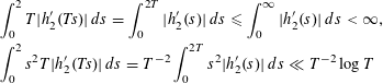 $$\begin{eqnarray}\displaystyle & & \displaystyle \displaystyle \int _{0}^{2}T|h_{2}^{\prime }(\mathit{Ts})|\,ds=\int _{0}^{2T}|h_{2}^{\prime }(s)|\,ds\leqslant \int _{0}^{\infty }|h_{2}^{\prime }(s)|\,ds<\infty ,\nonumber\\ \displaystyle & & \displaystyle \displaystyle \int _{0}^{2}s^{2}T|h_{2}^{\prime }(\mathit{Ts})|\,ds=T^{-2}\int _{0}^{2T}s^{2}|h_{2}^{\prime }(s)|\,ds\ll T^{-2}\log T\nonumber\end{eqnarray}$$
and
 $$\begin{eqnarray}\int _{0}^{2}s^{3}T|h_{2}^{\prime }(\mathit{Ts})|\,ds=T^{-3}\int _{0}^{2T}s^{3}|h_{2}^{\prime }(s)|\,ds\ll T^{-2}\end{eqnarray}$$
and therefore for
 $n$
satisfying
$n$
satisfying
 ${\mathcal{D}}(n,\unicode[STIX]{x1D716}/2),$
 $$\begin{eqnarray}\displaystyle \text{Err}(X_{\!f_{n},r}) & \ll & \displaystyle \cos ^{-2}\unicode[STIX]{x1D703}r^{4}(T^{-2}+\unicode[STIX]{x1D6E5}(n)+\widetilde{V}(\text{}\underline{v})T^{-2}\log T+\widetilde{V}(\text{}\underline{v})\unicode[STIX]{x1D6E5}(n)^{2})\nonumber\\ \displaystyle & \ll & \displaystyle \cos ^{-2}\unicode[STIX]{x1D703}r^{4} (T^{-2}+(\log n)^{-(1/2)\log (\unicode[STIX]{x1D70B}/2)+\unicode[STIX]{x1D716}/2}\nonumber\\ \displaystyle & & \displaystyle +\,\widetilde{V}(\text{}\underline{v})T^{-2}\log T+\widetilde{V}(\text{}\underline{v})(\log n)^{-\log (\unicode[STIX]{x1D70B}/2)+\unicode[STIX]{x1D716}} )\end{eqnarray}$$
Note that by (4.16), for Bourgain’s eigenfunctions, for almost all
 $n\in S_{2}$
, we have
$n\in S_{2}$
, we have
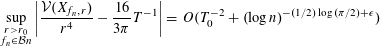 $$\begin{eqnarray}\sup _{\substack{ r>r_{0} \\ f_{n}\in {\mathcal{B}}n}}\bigg|\frac{\text{}{\mathcal{V}}\text{}(X_{\!f_{n},r})}{r^{4}}-\frac{16}{3\unicode[STIX]{x1D70B}}T^{-1}\bigg|=O(T_{0}^{-2}+(\log n)^{-(1/2)\log (\unicode[STIX]{x1D70B}/2)+\unicode[STIX]{x1D716}})\end{eqnarray}$$
for every
 $\unicode[STIX]{x1D716}>0$
and in particular
$\unicode[STIX]{x1D716}>0$
and in particular
 $$\begin{eqnarray}\displaystyle {\mathcal{V}}(X_{\!f_{n},r})=o(r^{4}) & & \displaystyle\end{eqnarray}$$
uniformly for
 $r>r_{0}$
for a density-1 sequence in
$r>r_{0}$
for a density-1 sequence in
 $S_{2}$
. Therefore, (4.17) serves as a refinement of [Reference Granville and Wigman14, Corollary 1.10] for this specific case (for a density-1 sequence in
$S_{2}$
. Therefore, (4.17) serves as a refinement of [Reference Granville and Wigman14, Corollary 1.10] for this specific case (for a density-1 sequence in
 $S_{2}$
), since [Reference Granville and Wigman14, Corollary 1.10] yields
$S_{2}$
), since [Reference Granville and Wigman14, Corollary 1.10] yields
 ${\mathcal{V}}(X_{\!f_{n},r})=o(r^{4})$
under the additional assumption
${\mathcal{V}}(X_{\!f_{n},r})=o(r^{4})$
under the additional assumption
 $T_{0}\gg n^{4\unicode[STIX]{x1D716}}$
.
$T_{0}\gg n^{4\unicode[STIX]{x1D716}}$
.
4.3 Proof of Proposition 4.5
In this section we prove Proposition 4.5. First, we define a binary relation on
 ${\mathcal{E}}_{n}$
.
${\mathcal{E}}_{n}$
.
Definition 4.6. For
 $\unicode[STIX]{x1D706}\neq -\unicode[STIX]{x1D706}^{\prime }\in {\mathcal{E}}_{n}$
, we say that
$\unicode[STIX]{x1D706}\neq -\unicode[STIX]{x1D706}^{\prime }\in {\mathcal{E}}_{n}$
, we say that
 $\unicode[STIX]{x1D706}\prec \unicode[STIX]{x1D706}^{\prime }$
if the arc on the circle
$\unicode[STIX]{x1D706}\prec \unicode[STIX]{x1D706}^{\prime }$
if the arc on the circle
 $\sqrt{n}{\mathcal{S}}^{1}$
that connects
$\sqrt{n}{\mathcal{S}}^{1}$
that connects
 $\unicode[STIX]{x1D706}$
to
$\unicode[STIX]{x1D706}$
to
 $\unicode[STIX]{x1D706}^{\prime }$
counter-clockwise to
$\unicode[STIX]{x1D706}^{\prime }$
counter-clockwise to
 $\unicode[STIX]{x1D706}^{\prime }$
is shorter than the arc that connects them clockwise to
$\unicode[STIX]{x1D706}^{\prime }$
is shorter than the arc that connects them clockwise to
 $\unicode[STIX]{x1D706}^{\prime }$
. Recall that
$\unicode[STIX]{x1D706}^{\prime }$
. Recall that
 $\unicode[STIX]{x1D706}_{+}$
is the clockwise nearest neighbour of
$\unicode[STIX]{x1D706}_{+}$
is the clockwise nearest neighbour of
 $\unicode[STIX]{x1D706}$
on
$\unicode[STIX]{x1D706}$
on
 $\sqrt{n}{\mathcal{S}}^{1}$
. The proof of Proposition 4.5 employs the following auxiliary lemma to be proved in §9, establishing (4.10) in the particular case
$\sqrt{n}{\mathcal{S}}^{1}$
. The proof of Proposition 4.5 employs the following auxiliary lemma to be proved in §9, establishing (4.10) in the particular case
 $|c_{\unicode[STIX]{x1D706}}|^{2}=1$
for every
$|c_{\unicode[STIX]{x1D706}}|^{2}=1$
for every
 $\unicode[STIX]{x1D706}\in {\mathcal{E}}_{n}$
.
$\unicode[STIX]{x1D706}\in {\mathcal{E}}_{n}$
.
Lemma 4.7. Fix
 $\unicode[STIX]{x1D706}^{\prime }\in {\mathcal{E}}_{n}.$
For
$\unicode[STIX]{x1D706}^{\prime }\in {\mathcal{E}}_{n}.$
For
 $0\leqslant s<2$
, we have
$0\leqslant s<2$
, we have
 $$\begin{eqnarray}\displaystyle \frac{1}{N}\cdot \#\{\unicode[STIX]{x1D706}\in {\mathcal{E}}_{n}:\,\unicode[STIX]{x1D706}\succcurlyeq \unicode[STIX]{x1D706}^{\prime },\Vert \widehat{\unicode[STIX]{x1D706}}-\widehat{\unicode[STIX]{x1D706}^{\prime }}\Vert \leqslant s\}=\frac{s}{2\unicode[STIX]{x1D70B}}+O(s^{3}+\unicode[STIX]{x1D6E5}(n)), & & \displaystyle\end{eqnarray}$$
where the constant involved in the “O”-notation in (4.18) is absolute.
Remark 4.8. The estimate (4.18) is also valid with “
 $\succ$
”, “
$\succ$
”, “
 $\preccurlyeq$
” or “
$\preccurlyeq$
” or “
 $\prec$
” in place of “
$\prec$
” in place of “
 $\succcurlyeq$
”.
$\succcurlyeq$
”.
We are now in a position to prove Proposition 4.5.
Proof of Proposition 4.5 assuming Lemma 4.7.
First, we write
 $$\begin{eqnarray}\displaystyle F(s)=\mathop{\sum }_{\unicode[STIX]{x1D706}^{\prime }\in {\mathcal{E}}_{n}}|c_{\unicode[STIX]{x1D706}^{\prime }}|^{2}\mathop{\sum }_{\substack{ \unicode[STIX]{x1D706}\in {\mathcal{E}}_{n} \\ \Vert \widehat{\unicode[STIX]{x1D706}}-\widehat{\unicode[STIX]{x1D706}^{\prime }}\Vert \leqslant s \\ \unicode[STIX]{x1D706}\preccurlyeq \unicode[STIX]{x1D706}^{\prime }}}|c_{\unicode[STIX]{x1D706}}|^{2}+\mathop{\sum }_{\unicode[STIX]{x1D706}^{\prime }\in {\mathcal{E}}_{n}}|c_{\unicode[STIX]{x1D706}^{\prime }}|^{2}\mathop{\sum }_{\substack{ \unicode[STIX]{x1D706}\in {\mathcal{E}}_{n} \\ \Vert \widehat{\unicode[STIX]{x1D706}}-\widehat{\unicode[STIX]{x1D706}^{\prime }}\Vert \leqslant s \\ \unicode[STIX]{x1D706}\succcurlyeq \unicode[STIX]{x1D706}^{\prime }}}|c_{\unicode[STIX]{x1D706}}|^{2}+O\bigg(\frac{A_{4}}{N}\bigg). & & \displaystyle \nonumber\\ \displaystyle & & \displaystyle\end{eqnarray}$$
Using summation by parts, we get that for every
 $\unicode[STIX]{x1D706}^{\prime }\in {\mathcal{E}}_{n}$
,
$\unicode[STIX]{x1D706}^{\prime }\in {\mathcal{E}}_{n}$
,
 $$\begin{eqnarray}\displaystyle \mathop{\sum }_{\substack{ \unicode[STIX]{x1D706}\in {\mathcal{E}}_{n} \\ \Vert \widehat{\unicode[STIX]{x1D706}}-\widehat{\unicode[STIX]{x1D706}^{\prime }}\Vert \leqslant s \\ \unicode[STIX]{x1D706}\preccurlyeq \unicode[STIX]{x1D706}^{\prime }}}|c_{\unicode[STIX]{x1D706}}|^{2} & = & \displaystyle |c_{\unicode[STIX]{x1D706}^{\prime }}|^{2}\cdot \#\{\unicode[STIX]{x1D706}\in {\mathcal{E}}_{n}:\,\unicode[STIX]{x1D706}\preccurlyeq \unicode[STIX]{x1D706}^{\prime },\Vert \widehat{\unicode[STIX]{x1D706}}-\widehat{\unicode[STIX]{x1D706}^{\prime }}\Vert \leqslant s\}\nonumber\\ \displaystyle & & \displaystyle -\mathop{\sum }_{\substack{ \unicode[STIX]{x1D706}\in {\mathcal{E}}_{n} \\ \Vert \widehat{\unicode[STIX]{x1D706}}-\widehat{\unicode[STIX]{x1D706}^{\prime }}\Vert \leqslant s \\ \unicode[STIX]{x1D706}\prec \unicode[STIX]{x1D706}^{\prime }}}\!(|c_{\unicode[STIX]{x1D706}_{+}}|^{2}-|c_{\unicode[STIX]{x1D706}}|^{2})\cdot \#\{\unicode[STIX]{x1D707}\in {\mathcal{E}}_{n}:\,\unicode[STIX]{x1D707}\preccurlyeq \unicode[STIX]{x1D706},\Vert \widehat{\unicode[STIX]{x1D707}}-\widehat{\unicode[STIX]{x1D706}^{\prime }}\Vert \leqslant s\}.\nonumber\\ \displaystyle & & \displaystyle\end{eqnarray}$$
By Lemma 4.7, the contribution of the first term on the right-hand side of (4.20) to
 $F(s)$
is
$F(s)$
is
 $$\begin{eqnarray}\displaystyle \mathop{\sum }_{\unicode[STIX]{x1D706}^{\prime }\in {\mathcal{E}}_{n}}|c_{\unicode[STIX]{x1D706}^{\prime }}|^{4}\cdot \#\{\unicode[STIX]{x1D706}\in {\mathcal{E}}_{n}:\,\unicode[STIX]{x1D706}\preccurlyeq \unicode[STIX]{x1D706}^{\prime },\Vert \widehat{\unicode[STIX]{x1D706}}-\widehat{\unicode[STIX]{x1D706}^{\prime }}\Vert \leqslant s\}=A_{4}\cdot (s/2\unicode[STIX]{x1D70B}+O(s^{3}+\unicode[STIX]{x1D6E5}(n))). & & \displaystyle \nonumber\\ \displaystyle & & \displaystyle\end{eqnarray}$$
The contribution of the sum on the right-hand side of (4.20) to
 $F(s)$
is
$F(s)$
is
 $$\begin{eqnarray}\displaystyle & & \displaystyle \mathop{\sum }_{\unicode[STIX]{x1D706}^{\prime }\in {\mathcal{E}}_{n}}|c_{\unicode[STIX]{x1D706}^{\prime }}|^{2}\mathop{\sum }_{\substack{ \unicode[STIX]{x1D706}\in {\mathcal{E}}_{n} \\ \Vert \widehat{\unicode[STIX]{x1D706}}-\widehat{\unicode[STIX]{x1D706}^{\prime }}\Vert \leqslant s \\ \unicode[STIX]{x1D706}\prec \unicode[STIX]{x1D706}^{\prime }}}(|c_{\unicode[STIX]{x1D706}_{+}}|^{2}-|c_{\unicode[STIX]{x1D706}}|^{2})\cdot \#\{\unicode[STIX]{x1D707}\in {\mathcal{E}}_{n}:\,\unicode[STIX]{x1D707}\preccurlyeq \unicode[STIX]{x1D706},\,\Vert \widehat{\unicode[STIX]{x1D707}}-\widehat{\unicode[STIX]{x1D706}^{\prime }}\Vert \leqslant s\}\nonumber\\ \displaystyle & & \displaystyle \quad \ll N(s+\unicode[STIX]{x1D6E5}(n))\mathop{\sum }_{\unicode[STIX]{x1D706}\in {\mathcal{E}}_{n}}||c_{\unicode[STIX]{x1D706}_{+}}|^{2}-|c_{\unicode[STIX]{x1D706}}|^{2}|\!\mathop{\sum }_{\substack{ \unicode[STIX]{x1D706}^{\prime }\in {\mathcal{E}}_{n} \\ \Vert \widehat{\unicode[STIX]{x1D706}}-\widehat{\unicode[STIX]{x1D706}^{\prime }}\Vert \leqslant s \\ \unicode[STIX]{x1D706}\prec \unicode[STIX]{x1D706}^{\prime }}}\!|c_{\unicode[STIX]{x1D706}^{\prime }}|^{2}\ll (s+\unicode[STIX]{x1D6E5}(n))^{2}[\text{}\underline{v}]_{\infty }V(\text{}\underline{v}).\nonumber\\ \displaystyle & & \displaystyle\end{eqnarray}$$
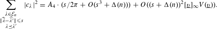 $$\begin{eqnarray}\displaystyle \mathop{\sum }_{\substack{ \unicode[STIX]{x1D706}\in {\mathcal{E}}_{n} \\ \Vert \widehat{\unicode[STIX]{x1D706}}-\widehat{\unicode[STIX]{x1D706}^{\prime }}\Vert \leqslant s \\ \unicode[STIX]{x1D706}\preccurlyeq \unicode[STIX]{x1D706}^{\prime }}}|c_{\unicode[STIX]{x1D706}}|^{2}=A_{4}\cdot (s/2\unicode[STIX]{x1D70B}+O(s^{3}+\unicode[STIX]{x1D6E5}(n)))+O((s+\unicode[STIX]{x1D6E5}(n))^{2}[\text{}\underline{v}]_{\infty }V(\text{}\underline{v})). & & \displaystyle \nonumber\\ \displaystyle & & \displaystyle\end{eqnarray}$$
By symmetry, the second summation in (4.19) obeys (4.20) with “
 $\succ$
”, “
$\succ$
”, “
 $\succcurlyeq$
” and
$\succcurlyeq$
” and
 $|c_{\unicode[STIX]{x1D706}_{-}}|^{2}$
in place of “
$|c_{\unicode[STIX]{x1D706}_{-}}|^{2}$
in place of “
 $\prec$
”, “
$\prec$
”, “
 $\preccurlyeq$
” and
$\preccurlyeq$
” and
 $|c_{\unicode[STIX]{x1D706}_{+}}|^{2}$
, where
$|c_{\unicode[STIX]{x1D706}_{+}}|^{2}$
, where
 $\unicode[STIX]{x1D706}_{-}$
is the counter-clockwise nearest neighbour to
$\unicode[STIX]{x1D706}_{-}$
is the counter-clockwise nearest neighbour to
 $\unicode[STIX]{x1D706}$
. The statement of Proposition 4.5 follows from the analogues of the estimates (4.21), (4.22) and (4.23).◻
$\unicode[STIX]{x1D706}$
. The statement of Proposition 4.5 follows from the analogues of the estimates (4.21), (4.22) and (4.23).◻
5 Proof of Theorem 2.5, part 2: Gaussian moments,
$d=2$

In this section we study the higher moments of
 $\hat{X}_{\!f_{n},r}$
defined in (1.17) and prove the second part of Theorem 2.5, also implying the second part of Theorem 1.1.
$\hat{X}_{\!f_{n},r}$
defined in (1.17) and prove the second part of Theorem 2.5, also implying the second part of Theorem 1.1.
The proof of the following lower bound for
 ${\mathcal{V}}(X_{\!f_{n},r})$
with
${\mathcal{V}}(X_{\!f_{n},r})$
with
 $f_{n}\in {\mathcal{F}}_{2}(n;T(n),\unicode[STIX]{x1D702}(n))$
goes along the same lines as the proof of the lower bound in Theorem 1.5 below.
$f_{n}\in {\mathcal{F}}_{2}(n;T(n),\unicode[STIX]{x1D702}(n))$
goes along the same lines as the proof of the lower bound in Theorem 1.5 below.
Lemma 5.1. In the setting of Theorem 2.5, part (2), we have
 $$\begin{eqnarray}\frac{{\mathcal{V}}(X_{\!f_{n},r})}{r^{4}}\gg T(n)^{-1-2\unicode[STIX]{x1D702}(n)}\end{eqnarray}$$
uniformly for
 $r_{0}<r<r_{1}$
and
$r_{0}<r<r_{1}$
and
 $f_{n}\in {\mathcal{F}}_{2}(n;T(n),\unicode[STIX]{x1D702}(n))$
.
$f_{n}\in {\mathcal{F}}_{2}(n;T(n),\unicode[STIX]{x1D702}(n))$
.
Before proceeding to the proof of Theorem 2.5, we introduce some notation.
Definition 5.2.
(1) Define the set of “admissible”
$2k$
-tuples of lattice points by (5.1)$$\begin{eqnarray}\displaystyle {\mathcal{A}}_{n}(2k)=\{(\unicode[STIX]{x1D706}_{1},\ldots ,\unicode[STIX]{x1D706}_{2k})\in {\mathcal{D}}_{n}(2k):\;\forall 1\leqslant i\leqslant k\;\unicode[STIX]{x1D706}_{2i-1}\neq -\unicode[STIX]{x1D706}_{2i}\}. & & \displaystyle \nonumber\\ \displaystyle & & \displaystyle\end{eqnarray}$$
(2) Given an admissible
$2k$
-tuple of lattice points
$(\unicode[STIX]{x1D706}_{1},\ldots ,\unicode[STIX]{x1D706}_{2k})\in {\mathcal{A}}_{n}(2k)$
, let
${\sim}$
be the equivalence relation on the set
$\{1,\ldots ,2k\}$
generated by:(a)
$2i-1\sim 2i$
for every
$1\leqslant i\leqslant k$
;(b)
$j\sim j^{\prime }$
if
$\unicode[STIX]{x1D706}_{j}+\unicode[STIX]{x1D706}_{j}^{\prime }=0$
.
Let
$\{\unicode[STIX]{x1D6EC}_{1},\ldots ,\unicode[STIX]{x1D6EC}_{m}\}$
be the partition of
$\{1,\ldots ,2k\}$
into equivalence classes of
${\sim}$
and denote
$l_{j}=\#\unicode[STIX]{x1D6EC}_{m}/2$
for
$1\leqslant j\leqslant m$
, so that
$\sum _{j=1}^{m}l_{j}=k$
; clearly,
$2\leqslant l_{j}\in \mathbb{Z}$
for every
$1\leqslant j\leqslant m$
. We call the multiset (5.2)the structure set of the$$\begin{eqnarray}\displaystyle S(\unicode[STIX]{x1D706}_{1},\ldots ,\unicode[STIX]{x1D706}_{2k}):=\{l_{1},\ldots ,l_{m}\} & & \displaystyle\end{eqnarray}$$
$2k$
-tuple
$(\unicode[STIX]{x1D706}_{1},\ldots ,\unicode[STIX]{x1D706}_{2k}).$


Recall that the moments of a standard Gaussian random variable
 $Z\sim N(0,1)$
are
$Z\sim N(0,1)$
are
 $$\begin{eqnarray}\mathbb{E}[Z^{k}]=\left\{\begin{array}{@{}ll@{}}(k-1)!!,\quad & k~\text{even},\\ 0,\quad & k~\text{odd}.\end{array}\right.\end{eqnarray}$$
We are now in a position to prove the second part of Theorem 2.5.
Proof of Theorem 2.5, part 2.
By the length-
 $2k$
diagonal domination assumption, we have
$2k$
diagonal domination assumption, we have
 $$\begin{eqnarray}\displaystyle \mathbb{E}[\hat{X}_{\!f_{n},r}^{k}] & = & \displaystyle (2\unicode[STIX]{x1D70B})^{k}r^{2k}{\mathcal{V}}(X_{\!f_{n},r})^{-k/2}\nonumber\\ \displaystyle & & \displaystyle \times \,\mathop{\sum }_{(\unicode[STIX]{x1D706}_{1},\ldots ,\unicode[STIX]{x1D706}_{2k})\in {\mathcal{A}}_{n}(2k)}\mathop{\prod }_{j=1}^{k}c_{\unicode[STIX]{x1D706}_{2j-1}}c_{\unicode[STIX]{x1D706}_{2j}}g_{2}(r\Vert \unicode[STIX]{x1D706}_{2j-1}+\unicode[STIX]{x1D706}_{2j}\Vert )\nonumber\\ \displaystyle & & \displaystyle +\,O({\mathcal{V}}(X_{\!f_{n},r})^{-k/2}[\text{}\underline{v}]_{\infty }^{k}r^{2k}N^{-\unicode[STIX]{x1D6FE}})\end{eqnarray}$$
for some
 $\unicode[STIX]{x1D6FE}>0.$
We can rearrange the summation in (5.3), first summing over all possible structure sets
$\unicode[STIX]{x1D6FE}>0.$
We can rearrange the summation in (5.3), first summing over all possible structure sets
 ${\mathcal{L}}=\{l_{1},\ldots ,l_{m}\}$
and then summing over the admissible
${\mathcal{L}}=\{l_{1},\ldots ,l_{m}\}$
and then summing over the admissible
 $2k$
-tuples
$2k$
-tuples
 $(\unicode[STIX]{x1D706}_{1},\ldots ,\unicode[STIX]{x1D706}_{2k})\in {\mathcal{E}}_{n}^{2k}$
with the given structure set
$(\unicode[STIX]{x1D706}_{1},\ldots ,\unicode[STIX]{x1D706}_{2k})\in {\mathcal{E}}_{n}^{2k}$
with the given structure set
 $S(\unicode[STIX]{x1D706}_{1},\ldots ,\unicode[STIX]{x1D706}_{2k})={\mathcal{L}}$
: let
$S(\unicode[STIX]{x1D706}_{1},\ldots ,\unicode[STIX]{x1D706}_{2k})={\mathcal{L}}$
: let
 $$\begin{eqnarray}\displaystyle S_{{\mathcal{L}}}:=\mathop{\sum }_{\substack{ (\unicode[STIX]{x1D706}_{1},\ldots ,\unicode[STIX]{x1D706}_{2k})\in {\mathcal{A}}_{n}(2k) \\ S(\unicode[STIX]{x1D706}_{1},\ldots ,\unicode[STIX]{x1D706}_{2k})={\mathcal{L}}}}\mathop{\prod }_{j=1}^{k}c_{\unicode[STIX]{x1D706}_{2j-1}}c_{\unicode[STIX]{x1D706}_{2j}}g_{2}(r\Vert \unicode[STIX]{x1D706}_{2j-1}+\unicode[STIX]{x1D706}_{2j}\Vert ), & & \displaystyle \nonumber\end{eqnarray}$$
so that we may rewrite the summation on the right-hand side of (5.3) as
 $$\begin{eqnarray}\displaystyle & & \displaystyle \mathop{\sum }_{(\unicode[STIX]{x1D706}_{1},\ldots ,\unicode[STIX]{x1D706}_{2k})\in {\mathcal{A}}_{n}(2k)}\mathop{\prod }_{j=1}^{k}c_{\unicode[STIX]{x1D706}_{2j-1}}c_{\unicode[STIX]{x1D706}_{2j}}g_{2}(r\Vert \unicode[STIX]{x1D706}_{2j-1}+\unicode[STIX]{x1D706}_{2j}\Vert )\nonumber\\ \displaystyle & & \displaystyle \quad =\mathop{\sum }_{\substack{ l_{1}+\cdots +l_{m}=k \\ l_{1},\ldots ,l_{m}\geqslant 2}}\mathop{\sum }_{\substack{ (\unicode[STIX]{x1D706}_{1},\ldots ,\unicode[STIX]{x1D706}_{2k})\in {\mathcal{A}}_{n}(2k) \\ S(\unicode[STIX]{x1D706}_{1},\ldots ,\unicode[STIX]{x1D706}_{2k})={\mathcal{L}}}}S_{{\mathcal{L}}}.\end{eqnarray}$$
For a fixed structure set
 ${\mathcal{L}}=\{l_{1},\ldots ,l_{m}\}$
, we have
${\mathcal{L}}=\{l_{1},\ldots ,l_{m}\}$
, we have
 $$\begin{eqnarray}\displaystyle S_{{\mathcal{L}}} & = & \displaystyle a({\mathcal{L}})\mathop{\prod }_{j=1}^{m}\mathop{\sum }_{\unicode[STIX]{x1D706}_{1},\ldots ,\unicode[STIX]{x1D706}_{l_{j}}\in {\mathcal{E}}_{n}}|c_{\unicode[STIX]{x1D706}_{1}}|^{2}g_{2}(r\Vert \unicode[STIX]{x1D706}_{l_{j}}-\unicode[STIX]{x1D706}_{1}\Vert )\mathop{\prod }_{i=1}^{l_{j}-1}|c_{\unicode[STIX]{x1D706}_{i+1}}|^{2}g_{2}(r\Vert \unicode[STIX]{x1D706}_{i}-\unicode[STIX]{x1D706}_{i+1}\Vert )\nonumber\\ \displaystyle & & \displaystyle +\,O([\text{}\underline{v}]_{\infty }^{k}N^{-1}),\end{eqnarray}$$
where
 $a({\mathcal{L}})$
is a constant depending on
$a({\mathcal{L}})$
is a constant depending on
 ${\mathcal{L}}$
; omitting the condition that the lattice points are distinct on the right-hand side of (5.5) that is absorbed within the error term in (5.5). Thus,
${\mathcal{L}}$
; omitting the condition that the lattice points are distinct on the right-hand side of (5.5) that is absorbed within the error term in (5.5). Thus,
 $$\begin{eqnarray}\displaystyle S_{{\mathcal{L}}} & \ll & \displaystyle [\text{}\underline{v}]_{\infty }^{k}N^{-k}\mathop{\prod }_{j=1}^{m}\mathop{\sum }_{\unicode[STIX]{x1D706}_{1}\in {\mathcal{E}}_{n}}\mathop{\sum }_{\unicode[STIX]{x1D706}_{2}\in {\mathcal{E}}_{n}}|g_{2}(r\Vert \unicode[STIX]{x1D706}_{2}-\unicode[STIX]{x1D706}_{1}\Vert )|\cdots \mathop{\sum }_{\unicode[STIX]{x1D706}_{l_{j}}\in {\mathcal{E}}_{n}}|g_{2}(r\Vert \unicode[STIX]{x1D706}_{l_{j}-1}-\unicode[STIX]{x1D706}_{l_{j}}\Vert )|\nonumber\\ \displaystyle & & \displaystyle +\,[\text{}\underline{v}]_{\infty }^{k}N^{-1}.\end{eqnarray}$$
Recall the definition of
 $F_{\unicode[STIX]{x1D706}_{0}}$
in (4.9). By Lemma 4.7, we have
$F_{\unicode[STIX]{x1D706}_{0}}$
in (4.9). By Lemma 4.7, we have
 $$\begin{eqnarray}\displaystyle F_{\unicode[STIX]{x1D706}_{0}}(s)=\frac{s}{\unicode[STIX]{x1D70B}}+O(s^{3}+\unicode[STIX]{x1D6E5}(n))=O(s+\unicode[STIX]{x1D6E5}(n)). & & \displaystyle\end{eqnarray}$$
Thus, by Lemma 4.3 and (5.7), we have that
 $$\begin{eqnarray}\displaystyle \frac{1}{N}\mathop{\sum }_{\unicode[STIX]{x1D706}\in {\mathcal{E}}_{n}}|g_{2}(r\Vert \unicode[STIX]{x1D706}-\unicode[STIX]{x1D706}_{0}\Vert )| & = & \displaystyle \int _{0}^{2}|g_{2}(\mathit{Ts})|\,dF_{\unicode[STIX]{x1D706}_{0}}(s)\nonumber\\ \displaystyle & = & \displaystyle |g_{2}(2T)|-\frac{1}{2N}+O\bigg(\int _{0}^{2}(s+\unicode[STIX]{x1D6E5}(n))T|g_{2}^{\prime }(\mathit{Ts})|\,ds\bigg)\nonumber\\ \displaystyle & = & \displaystyle O\bigg(T^{-3/2}+(\unicode[STIX]{x1D6E5}(n)+T^{-1})\int _{0}^{2T}|g_{2}^{\prime }(s)|\,ds\bigg)\nonumber\\ \displaystyle & = & \displaystyle O(T^{-1})\end{eqnarray}$$
for
 $n$
satisfying the hypothesis
$n$
satisfying the hypothesis
 ${\mathcal{D}}(n,\unicode[STIX]{x1D716})$
. Applying (5.8) to each of the
${\mathcal{D}}(n,\unicode[STIX]{x1D716})$
. Applying (5.8) to each of the
 $l_{j}-1$
inner summations in (5.6), we obtain
$l_{j}-1$
inner summations in (5.6), we obtain
 $$\begin{eqnarray}\displaystyle S_{{\mathcal{L}}}\ll [\text{}\underline{v}]_{\infty }^{k}N^{-k+m}\mathop{\prod }_{j=1}^{m}(NT^{-1})^{l_{j}-1}+[\text{}\underline{v}]_{\infty }^{k}N^{-1}\ll [\text{}\underline{v}]_{\infty }^{k}T^{-k+m}. & & \displaystyle \nonumber\end{eqnarray}$$
Let
 ${\mathcal{L}}_{0}=\{2,2,\ldots ,2\}$
. Note that if
${\mathcal{L}}_{0}=\{2,2,\ldots ,2\}$
. Note that if
 ${\mathcal{L}}\neq {\mathcal{L}}_{0}$
, then
${\mathcal{L}}\neq {\mathcal{L}}_{0}$
, then
 $m\leqslant (k-1)/2$
and therefore
$m\leqslant (k-1)/2$
and therefore
 $$\begin{eqnarray}\displaystyle S_{{\mathcal{L}}}=O([\text{}\underline{v}]_{\infty }^{k}T^{-(k+1)/2}). & & \displaystyle\end{eqnarray}$$
If
 $\{={\mathcal{L}}_{0}$
(this is a viable option for
$\{={\mathcal{L}}_{0}$
(this is a viable option for
 $k$
even), then
$k$
even), then
 $$\begin{eqnarray}\displaystyle S_{{\mathcal{L}}_{0}}=2^{k/2}(k-1)!!\bigg[\mathop{\sum }_{\unicode[STIX]{x1D706}_{1}\neq \unicode[STIX]{x1D706}_{2}\in {\mathcal{E}}_{n}}|c_{\unicode[STIX]{x1D706}_{1}}|^{2}|c_{\unicode[STIX]{x1D706}_{2}}|^{2}h_{2}(r\Vert \unicode[STIX]{x1D706}_{1}-\unicode[STIX]{x1D706}_{2}\Vert )\bigg]^{k/2}+O([\text{}\underline{v}]_{\infty }^{k}N^{-1}). & & \displaystyle \nonumber\\ \displaystyle & & \displaystyle\end{eqnarray}$$
By (4.5),
 $$\begin{eqnarray}\displaystyle \mathop{\sum }_{\unicode[STIX]{x1D706}_{1}\neq \unicode[STIX]{x1D706}_{2}\in {\mathcal{E}}_{n}}|c_{\unicode[STIX]{x1D706}_{1}}|^{2}|c_{\unicode[STIX]{x1D706}_{2}}|^{2}h_{2}(r\Vert \unicode[STIX]{x1D706}_{1}-\unicode[STIX]{x1D706}_{2}\Vert )=\frac{{\mathcal{V}}(X_{\!f_{n},r})}{8\unicode[STIX]{x1D70B}^{2}r^{4}}. & & \displaystyle\end{eqnarray}$$
Hence, (5.10) and (5.11) yield
 $$\begin{eqnarray}\displaystyle S_{{\mathcal{L}}_{0}}=(k-1)!!\bigg(\frac{{\mathcal{V}}(X_{\!f_{n},r})}{4\unicode[STIX]{x1D70B}^{2}r^{4}}\bigg)^{k/2}+O([\text{}\underline{v}]_{\infty }^{k}N^{-1}). & & \displaystyle\end{eqnarray}$$
Substituting (5.9) and (5.12) into (5.4) and applying Lemma 5.1, we finally obtain that for
 $k$
even,
$k$
even,
 $$\begin{eqnarray}\displaystyle |\mathbb{E}[\hat{X}_{\!f_{n},r}^{k}]-(k-1)!!|\ll T^{k\unicode[STIX]{x1D702}(n)}[\text{}\underline{v}]_{\infty }^{k}(T^{-1/2}+T^{k/2}N^{-\min \{1,\unicode[STIX]{x1D6FE}\}})\ll T^{-1/2+2k\unicode[STIX]{x1D702}(n)} & & \displaystyle \nonumber\end{eqnarray}$$
and, since for
 $k$
odd
$k$
odd
 ${\mathcal{L}}={\mathcal{L}}_{0}$
is not a viable option, we obtain
${\mathcal{L}}={\mathcal{L}}_{0}$
is not a viable option, we obtain
 $$\begin{eqnarray}\displaystyle \mathbb{E}[\hat{X}_{\!f_{n},r}^{k}]\ll T^{k\unicode[STIX]{x1D702}(n)}[\text{}\underline{v}]_{\infty }^{k}(T^{-1/2}+T^{k/2}N^{-\min \{1,\unicode[STIX]{x1D6FE}\}})\ll T^{-1/2+2k\unicode[STIX]{x1D702}(n)}; & & \displaystyle \nonumber\end{eqnarray}$$
the second part of Theorem 2.5 follows.◻
6 Proof of Theorem 1.3: asymptotics for the variance,
$d=3$

6.1 Proof of Theorem 1.3
Denote
 $$\begin{eqnarray}\displaystyle F_{3}(s)=\frac{1}{N^{2}}\cdot \#\{\unicode[STIX]{x1D706}\neq \unicode[STIX]{x1D706}^{\prime }\in {\mathcal{E}}_{n}:\Vert \widehat{\unicode[STIX]{x1D706}}-\widehat{\unicode[STIX]{x1D706}^{\prime }}\Vert \leqslant s\} & & \displaystyle\end{eqnarray}$$
(cf. (4.10)) and recall that the spherical cap discrepancy for the points in
 ${\mathcal{E}}_{n}$
is defined by
${\mathcal{E}}_{n}$
is defined by
 $$\begin{eqnarray}\displaystyle \unicode[STIX]{x1D6E5}_{3}(n)=\sup _{\substack{ x\in {\mathcal{S}}^{2} \\ 0<r\leqslant 2}}\bigg|\frac{1}{N}\cdot \#\{\unicode[STIX]{x1D706}\in {\mathcal{E}}_{n}:\,|\widehat{\unicode[STIX]{x1D706}}-x|\leqslant r\}-\frac{r^{2}}{4}\bigg|. & & \displaystyle\end{eqnarray}$$
Lemma 6.1. We have
 $$\begin{eqnarray}\displaystyle F_{3}(s)=\frac{s^{2}}{4}+O(\unicode[STIX]{x1D6E5}_{3}(n)). & & \displaystyle\end{eqnarray}$$
Proof. The estimate (6.3) follows immediately from the definition of the spherical cap discrepancy, since
 $$\begin{eqnarray}\displaystyle F_{3}(s)=\frac{1}{N}\mathop{\sum }_{\unicode[STIX]{x1D706}^{\prime }\in {\mathcal{E}}_{n}}\#\{\unicode[STIX]{x1D706}\in {\mathcal{E}}_{n}:\,0<\Vert \widehat{\unicode[STIX]{x1D706}}-\widehat{\unicode[STIX]{x1D706}^{\prime }}\Vert \leqslant s\}=\frac{s^{2}}{4}+O(\unicode[STIX]{x1D6E5}_{3}(n)).\Box & & \displaystyle \nonumber\end{eqnarray}$$
The discrepancy
 $\unicode[STIX]{x1D6E5}_{3}(n)$
satisfies
$\unicode[STIX]{x1D6E5}_{3}(n)$
satisfies
 $\unicode[STIX]{x1D6E5}_{3}(n)\leqslant n^{-\unicode[STIX]{x1D702}}$
for some small
$\unicode[STIX]{x1D6E5}_{3}(n)\leqslant n^{-\unicode[STIX]{x1D702}}$
for some small
 $\unicode[STIX]{x1D702}>0$
; see [Reference Bourgain, Rudnick and Sarnak8]. We are now in a position to prove Theorem 1.3.
$\unicode[STIX]{x1D702}>0$
; see [Reference Bourgain, Rudnick and Sarnak8]. We are now in a position to prove Theorem 1.3.
Proof of Theorem 1.3.
By (4.7), we have
 $$\begin{eqnarray}\displaystyle {\mathcal{V}}(X_{\!f_{n},r}) & = & \displaystyle 16\unicode[STIX]{x1D70B}^{3}r^{6}\frac{1}{N^{2}}\mathop{\sum }_{\substack{ \unicode[STIX]{x1D706},\unicode[STIX]{x1D706}^{\prime }\in {\mathcal{E}}_{n} \\ \unicode[STIX]{x1D706}\neq \unicode[STIX]{x1D706}^{\prime }}}h_{3}(T\Vert \widehat{\unicode[STIX]{x1D706}}-\widehat{\unicode[STIX]{x1D706}^{\prime }}\Vert )+O(r^{6}N^{-1/4+\unicode[STIX]{x1D716}}).\end{eqnarray}$$
For the summation in (6.4), we have
 $$\begin{eqnarray}\frac{1}{N^{2}}\mathop{\sum }_{\substack{ \unicode[STIX]{x1D706},\unicode[STIX]{x1D706}^{\prime }\in {\mathcal{E}}_{n} \\ \unicode[STIX]{x1D706}\neq \unicode[STIX]{x1D706}^{\prime }}}h_{3}(T\Vert \widehat{\unicode[STIX]{x1D706}}-\widehat{\unicode[STIX]{x1D706}^{\prime }}\Vert )=\int _{0}^{2}h_{3}(\mathit{Ts})\,dF_{3}(s).\end{eqnarray}$$
Thus, integrating by parts and using Lemma 6.1,
 $$\begin{eqnarray}\displaystyle \frac{1}{N^{2}}\mathop{\sum }_{\substack{ \unicode[STIX]{x1D706},\unicode[STIX]{x1D706}^{\prime }\in {\mathcal{E}}_{n} \\ \unicode[STIX]{x1D706}\neq \unicode[STIX]{x1D706}^{\prime }}}h_{3}(T\Vert \widehat{\unicode[STIX]{x1D706}}-\widehat{\unicode[STIX]{x1D706}^{\prime }}\Vert ) & = & \displaystyle h_{3}(2T)F_{3}(2)-\int _{0}^{2}F_{3}(s)\,dh_{3}(\mathit{Ts})\nonumber\\ \displaystyle & = & \displaystyle h_{3}(2T)F_{3}(2)-\frac{1}{4}\int _{0}^{2}s^{2}\,dh_{3}(\mathit{Ts})+\text{Err}(X_{\!f_{n},r}),\nonumber\\ \displaystyle & & \displaystyle\end{eqnarray}$$
where
 $$\begin{eqnarray}\displaystyle \text{Err}(X_{\!f_{n},r})\ll \unicode[STIX]{x1D6E5}_{3}(n)\int _{0}^{2}T|h_{3}^{\prime }(\mathit{Ts})|\,ds. & & \displaystyle\end{eqnarray}$$
Note that
 $h_{3}(s)\ll s^{-4}$
as
$h_{3}(s)\ll s^{-4}$
as
 $s\rightarrow \infty$
. Thus, integrating by parts, the main term on the right-hand side of (6.5) satisfies
$s\rightarrow \infty$
. Thus, integrating by parts, the main term on the right-hand side of (6.5) satisfies
 $$\begin{eqnarray}\displaystyle h_{3}(2T)F_{3}(2)-\frac{1}{4}\int _{0}^{2}s^{2}\,dh_{3}(\mathit{Ts})=\frac{1}{2}\int _{0}^{2}s\cdot h_{3}(\mathit{Ts})\,ds+O(T^{-4}), & & \displaystyle\end{eqnarray}$$
so that
 $$\begin{eqnarray}\displaystyle \int _{0}^{2}s\cdot h_{3}(\mathit{Ts})\,ds=\frac{1}{T^{2}}\int _{0}^{2T}s\cdot h_{3}(s)\,ds=\frac{1}{T^{2}}\int _{0}^{\infty }s\cdot h_{3}(s)\,ds+O(T^{-4}). & & \displaystyle \nonumber\\ \displaystyle & & \displaystyle\end{eqnarray}$$
A direct computation shows that
 $$\begin{eqnarray}\displaystyle \int _{0}^{\infty }s\cdot h_{3}(s)\,ds=\frac{1}{2\unicode[STIX]{x1D70B}^{3}}\int _{0}^{\infty }\frac{1}{s^{3}}\bigg(\frac{\sin s}{s}-\cos s\bigg)^{2}\,ds=(2\unicode[STIX]{x1D70B})^{-3} & & \displaystyle\end{eqnarray}$$
and, therefore, substituting (6.9) into (6.8) and then into (6.7), we get
 $$\begin{eqnarray}\displaystyle h_{3}(2T)F_{3}(2)-\frac{1}{4}\int _{0}^{2}s^{2}\,dh_{3}(\mathit{Ts})=\frac{1}{16\unicode[STIX]{x1D70B}^{3}}T^{-2}+O(T^{-4}). & & \displaystyle\end{eqnarray}$$
Note that
 $h_{3}^{\prime }(s)\ll (1+s^{4})^{-1}$
. Thus,
$h_{3}^{\prime }(s)\ll (1+s^{4})^{-1}$
. Thus,
 $$\begin{eqnarray}\displaystyle \int _{0}^{2}T|h_{3}^{\prime }(\mathit{Ts})|\,ds=\int _{0}^{2T}|h_{3}^{\prime }(s)|\,ds\leqslant \int _{0}^{\infty }|h_{3}^{\prime }(s)|\,ds<\infty & & \displaystyle\end{eqnarray}$$
and, therefore, substituting (6.11) into (6.6), we obtain
 $$\begin{eqnarray}\displaystyle \text{Err}(X_{\!f_{n},r})=O(\unicode[STIX]{x1D6E5}_{3}(n)). & & \displaystyle\end{eqnarray}$$
Substituting (6.12) into (6.10) and finally into (6.5), we obtain (1.21). ◻
Note that by (6.12),
 $$\begin{eqnarray}\sup _{\substack{ r>r_{0} \\ f_{n}\in {\mathcal{B}}n}}\bigg|\frac{{\mathcal{V}}(X_{\!f_{n},r})}{r^{6}}-T^{-2}\bigg|=O(T_{0}^{-4}+n^{-\unicode[STIX]{x1D702}})\end{eqnarray}$$
for every
 $n\not \equiv 0,4,7\,(8)$
and in particular
$n\not \equiv 0,4,7\,(8)$
and in particular
 $$\begin{eqnarray}{\mathcal{V}}(X_{\!f_{n},r})=o(r^{6})\end{eqnarray}$$
uniformly for
 $r>r_{0}$
for every
$r>r_{0}$
for every
 $n\not \equiv 0,4,7\,(8)$
.
$n\not \equiv 0,4,7\,(8)$
.
7 Proofs of Theorems 1.5 and 1.6
Proof of Theorems 1.5 and 1.6, upper bounds.
By substituting the bound
 $|c_{\unicode[STIX]{x1D706}}|^{2}\leqslant N^{-1+\unicode[STIX]{x1D716}}$
into (4.5), we have
$|c_{\unicode[STIX]{x1D706}}|^{2}\leqslant N^{-1+\unicode[STIX]{x1D716}}$
into (4.5), we have
 $$\begin{eqnarray}\displaystyle {\mathcal{V}}(X_{\!f_{n},r})\ll r^{4}N^{-1+\unicode[STIX]{x1D716}}\mathop{\sum }_{\unicode[STIX]{x1D706}_{0}\in {\mathcal{E}}_{n}}|c_{\unicode[STIX]{x1D706}_{0}}|^{2}\mathop{\sum }_{\unicode[STIX]{x1D706}\in {\mathcal{E}}_{n}}h_{2}(r\Vert \unicode[STIX]{x1D706}-\unicode[STIX]{x1D706}_{0}\Vert ). & & \displaystyle\end{eqnarray}$$
By Lemma 4.3 and (5.7), we have
 $$\begin{eqnarray}\displaystyle \frac{1}{N}\mathop{\sum }_{\unicode[STIX]{x1D706}\in {\mathcal{E}}_{n}}h_{2}(r\Vert \unicode[STIX]{x1D706}-\unicode[STIX]{x1D706}_{0}\Vert ) & = & \displaystyle \int _{0}^{2}h_{2}(\mathit{Ts})\,dF_{\unicode[STIX]{x1D706}_{0}}(s)\nonumber\\ \displaystyle & = & \displaystyle h_{2}(2T)-\frac{1}{4N}+O\bigg(\int _{0}^{2}(s+\unicode[STIX]{x1D6E5}(n))T|h_{2}^{\prime }(\mathit{Ts})|\,ds\bigg)\nonumber\\ \displaystyle & = & \displaystyle O(T^{-1}+(\log n)^{-(1/2)\log (\unicode[STIX]{x1D70B}/2)+\unicode[STIX]{x1D716}})\end{eqnarray}$$
for
 $n$
satisfying the hypothesis
$n$
satisfying the hypothesis
 ${\mathcal{D}}(n,\unicode[STIX]{x1D716})$
. Substituting (7.2) into (7.1), we get the upper bound in Theorem 1.5. The upper bound (1.26) in Theorem 1.6 follows along similar lines.◻
${\mathcal{D}}(n,\unicode[STIX]{x1D716})$
. Substituting (7.2) into (7.1), we get the upper bound in Theorem 1.5. The upper bound (1.26) in Theorem 1.6 follows along similar lines.◻
We now turn to proving the claimed lower bounds for the variance of
 $X_{\!f_{n},r}$
. First, we need the following lemma, proved at the end of §7.
$X_{\!f_{n},r}$
. First, we need the following lemma, proved at the end of §7.
Lemma 7.1.
(1) Let
$\{x_{m}\}_{m=1}^{M}$
be
$M$
points on the unit circle
${\mathcal{S}}^{1}.$
For every
$1<T<M/2$
, we have $$\begin{eqnarray}\#\{x_{i}\neq x_{j}:\,|x_{i}-x_{j}|\leqslant 1/T\}\gg M^{2}/T.\end{eqnarray}$$
(2) Let
$\{x_{m}\}_{m=1}^{M}$
be
$M$
points on the unit sphere
$S^{2}.$
For every
$1<T<\sqrt{M}/2$
, we have $$\begin{eqnarray}\#\{x_{i}\neq x_{j}:\,|x_{i}-x_{j}|\leqslant 1/T\}\gg M^{2}/T^{2}.\end{eqnarray}$$


We are now in a position to prove the lower bounds (1.25) and (1.26) of Theorems 1.5 and 1.6.
Proof of Theorems 1.5 and 1.6, lower bounds assuming Lemma 7.1.
For
 $d=2$
, we let
$d=2$
, we let
 $$\begin{eqnarray}R=\#\bigg\{\unicode[STIX]{x1D706}\in {\mathcal{E}}_{n}:\,|c_{\unicode[STIX]{x1D706}}|^{2}\geqslant \frac{1}{2N}\bigg\},\end{eqnarray}$$
so that
 $$\begin{eqnarray}1=\mathop{\sum }_{\unicode[STIX]{x1D706}\in {\mathcal{E}}_{n}}|c_{\unicode[STIX]{x1D706}}|^{2}=\mathop{\sum }_{\unicode[STIX]{x1D706}\in R}|c_{\unicode[STIX]{x1D706}}|^{2}+\mathop{\sum }_{\unicode[STIX]{x1D706}\notin R}|c_{\unicode[STIX]{x1D706}}|^{2}\leqslant N^{-1+\unicode[STIX]{x1D716}}\cdot \#R+1/2\end{eqnarray}$$
and hence
 $\#R\geqslant 2N^{1-\unicode[STIX]{x1D716}}.$
By the second part of Lemma 4.3, for
$\#R\geqslant 2N^{1-\unicode[STIX]{x1D716}}.$
By the second part of Lemma 4.3, for
 $c>0$
sufficiently small we have
$c>0$
sufficiently small we have
 $$\begin{eqnarray}\displaystyle {\mathcal{V}}(X_{\!f_{n},r}) & = & \displaystyle 8\unicode[STIX]{x1D70B}^{2}r^{4}\mathop{\sum }_{\substack{ \unicode[STIX]{x1D706},\unicode[STIX]{x1D706}^{\prime }\in {\mathcal{E}}_{n} \\ \unicode[STIX]{x1D706}\neq \unicode[STIX]{x1D706}^{\prime }}}|c_{\unicode[STIX]{x1D706}}|^{2}|c_{\unicode[STIX]{x1D706}^{\prime }}|^{2}h_{2}(T\Vert \widehat{\unicode[STIX]{x1D706}}-\widehat{\unicode[STIX]{x1D706}^{\prime }}\Vert )\nonumber\\ \displaystyle & \gg & \displaystyle r^{4}N^{-2}\mathop{\sum }_{\unicode[STIX]{x1D706}\neq \unicode[STIX]{x1D706}^{\prime }\in R}h_{2}(T\Vert \widehat{\unicode[STIX]{x1D706}}-\widehat{\unicode[STIX]{x1D706}^{\prime }}\Vert )\nonumber\\ \displaystyle & \gg & \displaystyle r^{4}N^{-2}\cdot \#\{\unicode[STIX]{x1D706}\neq \unicode[STIX]{x1D706}^{\prime }\in R:\,\Vert \widehat{\unicode[STIX]{x1D706}}-\widehat{\unicode[STIX]{x1D706}^{\prime }}\Vert \leqslant c/T\}.\nonumber\end{eqnarray}$$
By the first part of Lemma 7.1,
 $$\begin{eqnarray}{\mathcal{V}}(X_{\!f_{n},r})\gg r^{4}N^{-2}(\#R)^{2}T^{-1}\gg r^{4}N^{-2\unicode[STIX]{x1D716}}T^{-1}.\end{eqnarray}$$
The lower bound (1.26) of Theorem 1.6 follows along the same lines as the above, this time using the second part of Lemma 7.1 in place of the first one. ◻
Note that in the proof of the lower bound in Theorem 1.5, we have used the abundance of close-by pairs of lattice points with
 $|c_{\unicode[STIX]{x1D706}}|^{2}\geqslant 1/2N$
; in the absence of such close-by lattice points, the bound does not hold. For example, for
$|c_{\unicode[STIX]{x1D706}}|^{2}\geqslant 1/2N$
; in the absence of such close-by lattice points, the bound does not hold. For example, for
 $d=2$
, fix
$d=2$
, fix
 $\unicode[STIX]{x1D706}_{0}\in {\mathcal{E}}_{n}$
and let
$\unicode[STIX]{x1D706}_{0}\in {\mathcal{E}}_{n}$
and let
 $|c_{\pm \unicode[STIX]{x1D706}_{0}}|^{2}=1/2$
and
$|c_{\pm \unicode[STIX]{x1D706}_{0}}|^{2}=1/2$
and
 $c_{\unicode[STIX]{x1D706}}=0$
for every
$c_{\unicode[STIX]{x1D706}}=0$
for every
 $\unicode[STIX]{x1D706}\neq \pm \unicode[STIX]{x1D706}_{0}.$
Then
$\unicode[STIX]{x1D706}\neq \pm \unicode[STIX]{x1D706}_{0}.$
Then
 $$\begin{eqnarray}{\mathcal{V}}(X_{\!f_{n},r})=4\unicode[STIX]{x1D70B}^{2}r^{4}h_{2}(2T)\ll r^{4}T^{-3}.\end{eqnarray}$$
Proof of Lemma 7.1.
For the first part of Lemma 7.1, divide
 $S^{1}$
into
$S^{1}$
into
 $k=O(T)$
arcs
$k=O(T)$
arcs
 $I_{1},I_{2},\ldots ,I_{k}$
of length
$I_{1},I_{2},\ldots ,I_{k}$
of length
 ${<}1/T$
. For every
${<}1/T$
. For every
 $1\leqslant j\leqslant k,$
let
$1\leqslant j\leqslant k,$
let
 $n_{j}=\#\{m:\,x_{m}\in I_{j}\},$
so that
$n_{j}=\#\{m:\,x_{m}\in I_{j}\},$
so that
 $\sum _{j=1}^{k}n_{j}=M$
. By the Cauchy–Schwarz inequality,
$\sum _{j=1}^{k}n_{j}=M$
. By the Cauchy–Schwarz inequality,
 $$\begin{eqnarray}M^{2}=\bigg(\mathop{\sum }_{j=1}^{k}n_{j}\bigg)^{2}\leqslant k\mathop{\sum }_{j=1}^{k}n_{j}^{2}\ll T\mathop{\sum }_{j=1}^{k}n_{j}^{2}.\end{eqnarray}$$
Thus,
 $$\begin{eqnarray}\displaystyle \#\{x_{i}\neq x_{j}:\,|x_{i}-x_{j}|\leqslant 1/T\} & = & \displaystyle \#\{x_{i},x_{j}:\,|x_{i}-x_{j}|\leqslant 1/T\}-M\nonumber\\ \displaystyle & \gg & \displaystyle \mathop{\sum }_{j=1}^{k}n_{j}^{2}-M\gg M^{2}/T-M\gg M^{2}/T.\nonumber\end{eqnarray}$$
The second part of Lemma 7.1 is proved similarly. ◻
8 Restricted averages
8.1 Restricted moments
For
 $d=2$
, most of our principal results above are also valid in the more difficult scenario where
$d=2$
, most of our principal results above are also valid in the more difficult scenario where
 $x$
is drawn in
$x$
is drawn in
 $B_{x_{0}}(\unicode[STIX]{x1D70C})$
for some
$B_{x_{0}}(\unicode[STIX]{x1D70C})$
for some
 $x_{0}\in \mathbb{T}^{2}$
and
$x_{0}\in \mathbb{T}^{2}$
and
 $\unicode[STIX]{x1D70C}\gg n^{-1/2+o(1)}$
. In this case, the restricted moments are: expectation
$\unicode[STIX]{x1D70C}\gg n^{-1/2+o(1)}$
. In this case, the restricted moments are: expectation
 $$\begin{eqnarray}\displaystyle \mathbb{E}_{x_{0},\unicode[STIX]{x1D70C}}[X_{\!f_{n},r}]=\frac{1}{\operatorname{Vol}(B_{x_{0}}(\unicode[STIX]{x1D70C}))}\int _{B_{x_{0}}(\unicode[STIX]{x1D70C})}X_{\!f_{n},r;x}\,dx, & & \displaystyle\end{eqnarray}$$
higher centred moments
 $$\begin{eqnarray}\displaystyle & & \displaystyle \mathbb{E}_{x_{0},\unicode[STIX]{x1D70C}}[(X_{\!f_{n},r}-\mathbb{E}_{x_{0},\unicode[STIX]{x1D70C}}[X_{\!f_{n},r}])^{k}]\nonumber\\ \displaystyle & & \displaystyle \quad =\frac{1}{\operatorname{Vol}(B_{x_{0}}(\unicode[STIX]{x1D70C}))}\int _{B_{x_{0}}(\unicode[STIX]{x1D70C})}(X_{\!f_{n},r;x}-\mathbb{E}_{x_{0},\unicode[STIX]{x1D70C}}[X_{\!f_{n},r}])^{k}\,dx,\quad k\geqslant 2,\end{eqnarray}$$
and in particular the variance
 $$\begin{eqnarray}\displaystyle {\mathcal{V}}_{x_{0},\unicode[STIX]{x1D70C}}(X_{\!f_{n},r})=\mathbb{E}_{x_{0},\unicode[STIX]{x1D70C}}[(X_{\!f_{n},r}-\mathbb{E}_{x_{0},\unicode[STIX]{x1D70C}}[X_{\!f_{n},r}])^{2}]. & & \displaystyle\end{eqnarray}$$
We re-interpret the statement of Granville–Wigman’s [Reference Granville and Wigman14, Theorem 1.2] as evaluating the expected mass
 $$\begin{eqnarray}\mathbb{E}_{x_{0},\unicode[STIX]{x1D70C}}[X_{\!f_{n},r}]\sim \unicode[STIX]{x1D70B}r^{2},\end{eqnarray}$$
valid for almost all
 $n\in S_{2}$
, uniformly for
$n\in S_{2}$
, uniformly for
 $\unicode[STIX]{x1D70C}\gg n^{-1/2+o(1)}$
,
$\unicode[STIX]{x1D70C}\gg n^{-1/2+o(1)}$
,
 $x_{0}\in \mathbb{T}^{2}$
, and
$x_{0}\in \mathbb{T}^{2}$
, and
 $r>0$
(see the first part of Lemma 8.4).
$r>0$
(see the first part of Lemma 8.4).
8.2 Quasi-correlations
For the restricted moments (8.2) of
 $X_{\!f_{n},r}$
, one also needs to cope with quasi-correlations, i.e., tuples
$X_{\!f_{n},r}$
, one also needs to cope with quasi-correlations, i.e., tuples
 $(\unicode[STIX]{x1D706}^{1},\ldots ,\unicode[STIX]{x1D706}^{l})\in {\mathcal{E}}_{n}^{l}$
with the sum
$(\unicode[STIX]{x1D706}^{1},\ldots ,\unicode[STIX]{x1D706}^{l})\in {\mathcal{E}}_{n}^{l}$
with the sum
 $\sum _{i=1}^{l}\unicode[STIX]{x1D706}^{i}$
unexpectedly small, e.g. given a (small) fixed number
$\sum _{i=1}^{l}\unicode[STIX]{x1D706}^{i}$
unexpectedly small, e.g. given a (small) fixed number
 $\unicode[STIX]{x1D6FF}>0$
,
$\unicode[STIX]{x1D6FF}>0$
,
 $$\begin{eqnarray}\displaystyle \biggl\|\mathop{\sum }_{i=1}^{l}\unicode[STIX]{x1D706}^{i}\biggr\|<n^{1/2-\unicode[STIX]{x1D6FF}}; & & \displaystyle\end{eqnarray}$$
unlike the correlations (2.3), here there are no congruence obstructions, so that (8.4) makes sense with
 $l$
odd or even.
$l$
odd or even.
Definition 8.1 (Quasi-correlations; cf. [Reference Benatar, Marinucci and Wigman2, Definition 1.3]).
(1) For
$n\in S_{2}$
,
$l\in \mathbb{Z}_{{\geqslant}2}$
and
$0<K=K(n)<l\cdot n^{1/2}$
, define the set of length-
$l$
spectral quasi-correlations (8.5)$$\begin{eqnarray}\displaystyle {\mathcal{C}}_{n}(l;K)=\bigg\{(\unicode[STIX]{x1D706}^{1},\ldots ,\unicode[STIX]{x1D706}^{l})\in {\mathcal{E}}_{n}^{l}:\,0<\biggl\|\mathop{\sum }_{j=1}^{l}\unicode[STIX]{x1D706}^{j}\biggr\|\leqslant K\bigg\}. & & \displaystyle\end{eqnarray}$$
(2) Given
$\unicode[STIX]{x1D6FF}>0$
, we say that
$n\in S_{2}$
satisfies the
$(l,\unicode[STIX]{x1D6FF})$
-separateness hypothesis
${\mathcal{A}}(n;l,\unicode[STIX]{x1D6FF})$
if (8.6)$$\begin{eqnarray}\displaystyle {\mathcal{C}}_{n}(l;n^{1/2-\unicode[STIX]{x1D6FF}})=\varnothing . & & \displaystyle\end{eqnarray}$$


For example,
 ${\mathcal{A}}(n;2,\unicode[STIX]{x1D6FF})$
is equivalent to the aforementioned Bourgain–Rudnick separateness, satisfied [Reference Bourgain and Rudnick7, Lemma 5] by a density-
${\mathcal{A}}(n;2,\unicode[STIX]{x1D6FF})$
is equivalent to the aforementioned Bourgain–Rudnick separateness, satisfied [Reference Bourgain and Rudnick7, Lemma 5] by a density-
 $1$
sequence
$1$
sequence
 $S_{2}^{\prime }\subseteq S_{2}$
. More generally, it was shown in [Reference Benatar, Marinucci and Wigman2] that for every
$S_{2}^{\prime }\subseteq S_{2}$
. More generally, it was shown in [Reference Benatar, Marinucci and Wigman2] that for every
 $\unicode[STIX]{x1D6FF}>0$
and
$\unicode[STIX]{x1D6FF}>0$
and
 $l\geqslant 2$
, the assumption
$l\geqslant 2$
, the assumption
 ${\mathcal{A}}(n;l,\unicode[STIX]{x1D6FF})$
is satisfied by generic
${\mathcal{A}}(n;l,\unicode[STIX]{x1D6FF})$
is satisfied by generic
 $n\in S_{2}^{\prime }(l,\unicode[STIX]{x1D6FF})$
and hence a standard diagonal argument yields a density-
$n\in S_{2}^{\prime }(l,\unicode[STIX]{x1D6FF})$
and hence a standard diagonal argument yields a density-
 $1$
sequence
$1$
sequence
 $S_{2}^{\prime }\subseteq S_{2}$
so that
$S_{2}^{\prime }\subseteq S_{2}$
so that
 ${\mathcal{A}}(n;l,\unicode[STIX]{x1D6FF})$
is satisfied for all
${\mathcal{A}}(n;l,\unicode[STIX]{x1D6FF})$
is satisfied for all
 $l\geqslant 2$
and
$l\geqslant 2$
and
 $\unicode[STIX]{x1D6FF}>0$
for
$\unicode[STIX]{x1D6FF}>0$
for
 $n\in S_{2}^{\prime }$
sufficiently large.
$n\in S_{2}^{\prime }$
sufficiently large.
Theorem 8.2 [Reference Benatar, Marinucci and Wigman2].
For every fixed
 $l\geqslant 2$
and
$l\geqslant 2$
and
 $\unicode[STIX]{x1D6FF}>0$
, there exists a set
$\unicode[STIX]{x1D6FF}>0$
, there exists a set
 $S_{2}^{\prime }(l,\unicode[STIX]{x1D6FF})\subseteq S_{2}$
such that:
$S_{2}^{\prime }(l,\unicode[STIX]{x1D6FF})\subseteq S_{2}$
such that:
(1) the set
$S_{2}^{\prime }(l,\unicode[STIX]{x1D6FF})$
has density
$1$
in
$S_{2}$
;(2) for every
$n\in S_{2}^{\prime }(l,\unicode[STIX]{x1D6FF})$
, the length-
$l$
spectral quasi-correlation set is empty, i.e., the$$\begin{eqnarray}{\mathcal{C}}_{n}(l;n^{1/2-\unicode[STIX]{x1D6FF}})=\varnothing\end{eqnarray}$$
$(l,\unicode[STIX]{x1D6FF})$
-separateness hypothesis
${\mathcal{A}}(n;l,\unicode[STIX]{x1D6FF})$
is satisfied.


8.3 A version of Theorem 2.5 with restricted averages
We have the following analogue of Theorem 2.5.
Theorem 8.3. Let
 $\unicode[STIX]{x1D6FF}>0$
and
$\unicode[STIX]{x1D6FF}>0$
and
 $0<\unicode[STIX]{x1D716}<\unicode[STIX]{x1D6FF}/5$
.
$0<\unicode[STIX]{x1D716}<\unicode[STIX]{x1D6FF}/5$
.
(1) If
$S_{2}^{\prime }\subseteq S_{2}$
is a sequence satisfying the hypotheses
${\mathcal{D}}(n,\unicode[STIX]{x1D716}/2)$
,
${\mathcal{A}}(n;2,\unicode[STIX]{x1D716})$
and
${\mathcal{A}}(n;4,\unicode[STIX]{x1D716})$
for all
$n\in S_{2}^{\prime }$
, then in the setting of Theorem 2.5, part (1), uniformly for all$$\begin{eqnarray}{\mathcal{V}}_{x_{0},\unicode[STIX]{x1D70C}}(X_{\!f_{n},r})\sim \frac{16}{3\unicode[STIX]{x1D70B}\cos ^{2}\unicode[STIX]{x1D703}_{f_{n}}}r^{4}T^{-1}\end{eqnarray}$$
$x_{0}\in \mathbb{T}^{2}$
,
$n^{-1/2+\unicode[STIX]{x1D6FF}}\leqslant \unicode[STIX]{x1D70C}\leqslant 1$
and
$r_{0}<r<r_{1}$
, and
$f_{n}\in {\mathcal{F}}_{1}(n;T(n),\unicode[STIX]{x1D702}(n))$
.(2) Let
$k\geqslant 3$
be an integer. If
$S_{2}^{\prime }\subseteq S_{2}$
is a sequence satisfying the length-
$2k$
diagonal domination assumption and the hypotheses
${\mathcal{D}}(n,\unicode[STIX]{x1D716}),$
${\mathcal{A}}(n;2,\unicode[STIX]{x1D716})$
,
${\mathcal{A}}(n;4,\unicode[STIX]{x1D716})$
and
${\mathcal{A}}(n;2k,\unicode[STIX]{x1D716})$
for all
$n\in S_{2}^{\prime }$
, then in the setting of Theorem 2.5, part (2), uniformly for$$\begin{eqnarray}\mathbb{E}_{x_{0},\unicode[STIX]{x1D70C}}[\hat{X}_{\!f_{n},r}^{k}]\rightarrow \mathbb{E}[Z^{k}]\end{eqnarray}$$
$x_{0}\in \mathbb{T}^{2}$
,
$r_{0}<r<r_{1}$
,
$n^{-1/2+\unicode[STIX]{x1D6FF}}\leqslant \unicode[STIX]{x1D70C}\leqslant 1$
and
$f_{n}\in {\mathcal{F}}_{2}(n;T(n),\unicode[STIX]{x1D702}(n))$
, where
$Z\sim N(0,1)$
is the standard Gaussian variable.


Theorem 8.3 follows along similar lines as the proof of Theorem 2.5, where we use the expressions for the restricted moments below (cf. equation (4.1), Lemma 4.2 and equation (5.3)). We remark that Theorem 1.5 can also be extended to
 ${\mathcal{V}}_{x_{0},\unicode[STIX]{x1D70C}}(X_{\!f_{n},r})$
; however, the lower bound will only hold for a generic
${\mathcal{V}}_{x_{0},\unicode[STIX]{x1D70C}}(X_{\!f_{n},r})$
; however, the lower bound will only hold for a generic
 $n\in S_{2}$
.
$n\in S_{2}$
.
Lemma 8.4 (Expectation and variance,
$d=2$
,
$x$
drawn in shrinking discs).


For
 $d=2$
let
$d=2$
let
 $0<\unicode[STIX]{x1D6FF}<1/2$
,
$0<\unicode[STIX]{x1D6FF}<1/2$
,
 $0<\unicode[STIX]{x1D716}<\unicode[STIX]{x1D6FF}/5$
and
$0<\unicode[STIX]{x1D716}<\unicode[STIX]{x1D6FF}/5$
and
 $S_{2}^{\prime }\subseteq S_{2}$
.
$S_{2}^{\prime }\subseteq S_{2}$
.
(1) If
$n\in S_{2}^{\prime }$
satisfies the hypothesis
${\mathcal{A}}(n;2,\unicode[STIX]{x1D716})$
, then uniformly for$$\begin{eqnarray}\mathbb{E}_{x_{0},\unicode[STIX]{x1D70C}}[X_{\!f_{n},r}]=\unicode[STIX]{x1D70B}r^{2}+O(r^{2}n^{-(3/5)\unicode[STIX]{x1D6FF}+3\unicode[STIX]{x1D716}})\end{eqnarray}$$
$x_{0}\in \mathbb{T}^{2},$
$n^{-1/2+\unicode[STIX]{x1D6FF}}\leqslant \unicode[STIX]{x1D70C}\leqslant 1$
and
$r>0$
.(2) If
$n\in S_{2}^{\prime }$
satisfies the hypotheses
${\mathcal{A}}(n;2,\unicode[STIX]{x1D716})$
and
${\mathcal{A}}(n;4,\unicode[STIX]{x1D716})$
, then uniformly for$$\begin{eqnarray}\displaystyle {\mathcal{V}}_{x_{0},\unicode[STIX]{x1D70C}}(X_{\!f_{n},r})=8\unicode[STIX]{x1D70B}^{2}r^{4}\mathop{\sum }_{\substack{ \unicode[STIX]{x1D706},\unicode[STIX]{x1D706}^{\prime }\in {\mathcal{E}}_{n} \\ \unicode[STIX]{x1D706}\neq \unicode[STIX]{x1D706}^{\prime }}}|c_{\unicode[STIX]{x1D706}}|^{2}|c_{\unicode[STIX]{x1D706}^{\prime }}|^{2}h_{2}(r\Vert \unicode[STIX]{x1D706}-\unicode[STIX]{x1D706}^{\prime }\Vert )+O(r^{4}n^{-(3/5)\unicode[STIX]{x1D6FF}+4\unicode[STIX]{x1D716}}) & & \displaystyle \nonumber\end{eqnarray}$$
$x_{0}\in \mathbb{T}^{2},$
$n^{-1/2+\unicode[STIX]{x1D6FF}}\leqslant \unicode[STIX]{x1D70C}\leqslant 1$
and
$r>0$
.


Lemma 8.5 (Higher moments,
$d=2$
,
$x$
drawn in shrinking discs).


For
 $d=2$
, let
$d=2$
, let
 $k\geqslant 3$
,
$k\geqslant 3$
,
 $0<\unicode[STIX]{x1D6FF}<1/2$
,
$0<\unicode[STIX]{x1D6FF}<1/2$
,
 $0<\unicode[STIX]{x1D716}<\unicode[STIX]{x1D6FF}/5$
and
$0<\unicode[STIX]{x1D716}<\unicode[STIX]{x1D6FF}/5$
and
 $S_{2}^{\prime }\subseteq S_{2}$
satisfying
$S_{2}^{\prime }\subseteq S_{2}$
satisfying
 ${\mathcal{A}}(2;n,\unicode[STIX]{x1D716}),$
 ${\mathcal{A}}(4;n,\unicode[STIX]{x1D716}),$
and
${\mathcal{A}}(4;n,\unicode[STIX]{x1D716}),$
and
 ${\mathcal{A}}(n;2k,\unicode[STIX]{x1D716})$
for every
${\mathcal{A}}(n;2k,\unicode[STIX]{x1D716})$
for every
 $n\in S_{2}^{\prime }$
. We have
$n\in S_{2}^{\prime }$
. We have
 $$\begin{eqnarray}\displaystyle \mathbb{E}_{x_{0},\unicode[STIX]{x1D70C}}[\hat{X}_{\!f_{n},r}^{k}] & = & \displaystyle (2\unicode[STIX]{x1D70B})^{k}r^{2k}{\mathcal{V}}_{x_{0},\unicode[STIX]{x1D70C}}(X_{\!f_{n},r})^{-k/2}\nonumber\\ \displaystyle & & \displaystyle \times \,\mathop{\sum }_{\substack{ \forall 1\leqslant i\leqslant k,\,\unicode[STIX]{x1D706}_{i}\neq \unicode[STIX]{x1D706}_{i}^{\prime }\in {\mathcal{E}}_{n} \\ \mathop{\sum }_{i=1}^{k}(\unicode[STIX]{x1D706}_{i}-\unicode[STIX]{x1D706}_{i}^{\prime })=0}}\mathop{\prod }_{j=1}^{k}c_{\unicode[STIX]{x1D706}_{j}}\overline{c_{\unicode[STIX]{x1D706}_{j}^{\prime }}}g_{2}(r\Vert \unicode[STIX]{x1D706}_{j}-\unicode[STIX]{x1D706}_{j}^{\prime }\Vert )\nonumber\\ \displaystyle & & \displaystyle +\,O({\mathcal{V}}_{x_{0},\unicode[STIX]{x1D70C}}(X_{\!f_{n},r})^{-k/2}r^{2k}n^{-(3/5)\unicode[STIX]{x1D6FF}+4\unicode[STIX]{x1D716}})\nonumber\end{eqnarray}$$
uniformly for
 $x_{0}\in \mathbb{T}^{2},$
 $n^{-1/2+\unicode[STIX]{x1D6FF}}\leqslant \unicode[STIX]{x1D70C}\leqslant 1$
and
$n^{-1/2+\unicode[STIX]{x1D6FF}}\leqslant \unicode[STIX]{x1D70C}\leqslant 1$
and
 $r>0$
.
$r>0$
.
8.4 Proofs of Lemmas 8.4 and 8.5
Proof of Lemma 8.4, first part.
We have
 $$\begin{eqnarray}\displaystyle \mathbb{E}_{x_{0},\unicode[STIX]{x1D70C}}[X_{\!f_{n},r}]=\frac{1}{\unicode[STIX]{x1D70B}\unicode[STIX]{x1D70C}^{2}}\int _{B_{x_{0}}(\unicode[STIX]{x1D70C})}\int _{B_{x}(r)}f_{n}(y)^{2}\,dy\,dx. & & \displaystyle\end{eqnarray}$$
Theorem 1.2 of Granville–Wigman [Reference Granville and Wigman14] asserts that for
 $\unicode[STIX]{x1D716}_{1}>\unicode[STIX]{x1D716}_{2}>0$
,
$\unicode[STIX]{x1D716}_{1}>\unicode[STIX]{x1D716}_{2}>0$
,
 $0<\unicode[STIX]{x1D716}_{3}<\unicode[STIX]{x1D716}_{1}-\unicode[STIX]{x1D716}_{2}$
and
$0<\unicode[STIX]{x1D716}_{3}<\unicode[STIX]{x1D716}_{1}-\unicode[STIX]{x1D716}_{2}$
and
 $n\in S_{2}$
satisfying
$n\in S_{2}$
satisfying
 ${\mathcal{A}}(n;2,\unicode[STIX]{x1D716}_{2})$
, we have
${\mathcal{A}}(n;2,\unicode[STIX]{x1D716}_{2})$
, we have
 $$\begin{eqnarray}\displaystyle \int _{B_{x}(r)}f_{n}(y)^{2}\,dy=\unicode[STIX]{x1D70B}r^{2}(1+O(n^{-3\unicode[STIX]{x1D716}_{3}/2})) & & \displaystyle\end{eqnarray}$$
uniformly in
 $x\in \mathbb{T}^{2}$
and
$x\in \mathbb{T}^{2}$
and
 $r>n^{-1/2+\unicode[STIX]{x1D716}_{1}}$
. If
$r>n^{-1/2+\unicode[STIX]{x1D716}_{1}}$
. If
 $r>n^{-1/2+(2/5)\unicode[STIX]{x1D6FF}}$
, then by substituting (8.8) with
$r>n^{-1/2+(2/5)\unicode[STIX]{x1D6FF}}$
, then by substituting (8.8) with
 $\unicode[STIX]{x1D716}_{1}=\frac{2}{5}\unicode[STIX]{x1D6FF}$
,
$\unicode[STIX]{x1D716}_{1}=\frac{2}{5}\unicode[STIX]{x1D6FF}$
,
 $\unicode[STIX]{x1D716}_{2}=\unicode[STIX]{x1D716}$
and
$\unicode[STIX]{x1D716}_{2}=\unicode[STIX]{x1D716}$
and
 $\unicode[STIX]{x1D716}_{3}=\frac{2}{5}\unicode[STIX]{x1D6FF}-2\unicode[STIX]{x1D716}$
into (8.7), we have
$\unicode[STIX]{x1D716}_{3}=\frac{2}{5}\unicode[STIX]{x1D6FF}-2\unicode[STIX]{x1D716}$
into (8.7), we have
 $$\begin{eqnarray}\mathbb{E}_{x_{0},\unicode[STIX]{x1D70C}}[X_{\!f_{n},r}]=\unicode[STIX]{x1D70B}r^{2}(1+O(n^{-(3/2)((2/5)\unicode[STIX]{x1D6FF}-2\unicode[STIX]{x1D716})}))\end{eqnarray}$$
for every
 $\unicode[STIX]{x1D70C}$
.
$\unicode[STIX]{x1D70C}$
.
Otherwise, note that
 $$\begin{eqnarray}\mathbb{E}_{x_{0},\unicode[STIX]{x1D70C}}[X_{\!f_{n},r}]=\frac{1}{\unicode[STIX]{x1D70B}\unicode[STIX]{x1D70C}^{2}}\int _{B_{x_{0}}(\unicode[STIX]{x1D70C}+r)}f_{n}(y)^{2}\int _{B_{x_{0}}(\unicode[STIX]{x1D70C})\cap B_{y}(r)}\,dx\,dy,\end{eqnarray}$$
so
 $$\begin{eqnarray}\displaystyle \frac{r^{2}}{\unicode[STIX]{x1D70C}^{2}}\int _{B_{x_{0}}(\unicode[STIX]{x1D70C}-r)}f_{n}(y)^{2}\,dy\leqslant \mathbb{E}_{x_{0},\unicode[STIX]{x1D70C}}[X_{\!f_{n},r}]\leqslant \frac{r^{2}}{\unicode[STIX]{x1D70C}^{2}}\int _{B_{x_{0}}(\unicode[STIX]{x1D70C}+r)}f_{n}(y)^{2}\,dy. & & \displaystyle\end{eqnarray}$$
Since
 $r/\unicode[STIX]{x1D70C}\leqslant n^{-(3/5)\unicode[STIX]{x1D6FF}}$
, we can use (8.8) with
$r/\unicode[STIX]{x1D70C}\leqslant n^{-(3/5)\unicode[STIX]{x1D6FF}}$
, we can use (8.8) with
 $\unicode[STIX]{x1D716}_{1}=\unicode[STIX]{x1D6FF}$
,
$\unicode[STIX]{x1D716}_{1}=\unicode[STIX]{x1D6FF}$
,
 $\unicode[STIX]{x1D716}_{2}=\unicode[STIX]{x1D716}$
and
$\unicode[STIX]{x1D716}_{2}=\unicode[STIX]{x1D716}$
and
 $\unicode[STIX]{x1D716}_{3}=\unicode[STIX]{x1D6FF}-2\unicode[STIX]{x1D716}$
to deduce that
$\unicode[STIX]{x1D716}_{3}=\unicode[STIX]{x1D6FF}-2\unicode[STIX]{x1D716}$
to deduce that
 $$\begin{eqnarray}\displaystyle \int _{B_{x_{0}}(\unicode[STIX]{x1D70C}\pm r)}f_{n}(y)^{2}\,dy=\unicode[STIX]{x1D70B}\unicode[STIX]{x1D70C}^{2}(1+O(n^{-(3/5)\unicode[STIX]{x1D6FF}})) & & \displaystyle\end{eqnarray}$$
and the statement of the first part of Lemma 8.4 follows upon substituting (8.10) into (8.9). ◻
Proof of Lemma 8.4, second part.
We have
 $$\begin{eqnarray}{\mathcal{V}}_{x_{0},\unicode[STIX]{x1D70C}}(X_{\!f_{n},r})=\frac{1}{\unicode[STIX]{x1D70B}\unicode[STIX]{x1D70C}^{2}}\int _{B_{x_{0}}(\unicode[STIX]{x1D70C})}\bigg(\int _{B_{x}(r)}f_{n}(y)^{2}\,dy-\mathbb{E}_{x_{0},\unicode[STIX]{x1D70C}}[X_{\!f_{n},r}]\bigg)^{2}\,dx.\end{eqnarray}$$
By (4.3),
 $$\begin{eqnarray}\displaystyle & & \displaystyle \frac{1}{\unicode[STIX]{x1D70B}\unicode[STIX]{x1D70C}^{2}}\int _{B_{x_{0}}(\unicode[STIX]{x1D70C})}\bigg(\int _{B_{x}(r)}f_{n}(y)^{2}\,dy-\unicode[STIX]{x1D70B}r^{2}\bigg)^{2}\,dx\nonumber\\ \displaystyle & & \displaystyle \quad =4\unicode[STIX]{x1D70B}^{2}r^{4}\mathop{\sum }_{\substack{ \unicode[STIX]{x1D706},\unicode[STIX]{x1D706}^{\prime },\unicode[STIX]{x1D706}^{\prime \prime },\unicode[STIX]{x1D706}^{\prime \prime \prime }\in {\mathcal{E}}_{n} \\ \unicode[STIX]{x1D706}\neq \unicode[STIX]{x1D706}^{\prime } \\ \unicode[STIX]{x1D706}^{\prime \prime }\neq \unicode[STIX]{x1D706}^{\prime \prime \prime }}}c_{\unicode[STIX]{x1D706}}\overline{c_{\unicode[STIX]{x1D706}^{\prime }}}c_{\unicode[STIX]{x1D706}^{\prime \prime }}\overline{c_{\unicode[STIX]{x1D706}^{\prime \prime \prime }}}g_{2}(r\Vert \unicode[STIX]{x1D706}-\unicode[STIX]{x1D706}^{\prime }\Vert )g_{2}(r\Vert \unicode[STIX]{x1D706}^{\prime \prime }-\unicode[STIX]{x1D706}^{\prime \prime \prime }\Vert )\nonumber\\ \displaystyle & & \displaystyle \qquad \times \,\frac{1}{\unicode[STIX]{x1D70B}\unicode[STIX]{x1D70C}^{2}}\int _{B_{x_{0}}(\unicode[STIX]{x1D70C})}\text{e}(\langle x,\unicode[STIX]{x1D706}-\unicode[STIX]{x1D706}^{\prime }+\unicode[STIX]{x1D706}^{\prime \prime }-\unicode[STIX]{x1D706}^{\prime \prime \prime }\rangle )\,dx\nonumber\\ \displaystyle & & \displaystyle \quad =8\unicode[STIX]{x1D70B}^{2}r^{4}\mathop{\sum }_{\substack{ \unicode[STIX]{x1D706},\unicode[STIX]{x1D706}^{\prime }\in {\mathcal{E}}_{n} \\ \unicode[STIX]{x1D706}\neq \unicode[STIX]{x1D706}^{\prime }}}|c_{\unicode[STIX]{x1D706}}|^{2}|c_{\unicode[STIX]{x1D706}^{\prime }}|^{2}g_{2}(r\Vert \unicode[STIX]{x1D706}-\unicode[STIX]{x1D706}^{\prime }\Vert )^{2}\nonumber\\ \displaystyle & & \displaystyle \qquad +\,8\unicode[STIX]{x1D70B}^{2}r^{4}\mathop{\sum }_{\substack{ \unicode[STIX]{x1D706},\unicode[STIX]{x1D706}^{\prime },\unicode[STIX]{x1D706}^{\prime \prime },\unicode[STIX]{x1D706}^{\prime \prime \prime }\in {\mathcal{E}}_{n} \\ \unicode[STIX]{x1D706}\neq \unicode[STIX]{x1D706}^{\prime } \\ \unicode[STIX]{x1D706}^{\prime \prime }\neq \unicode[STIX]{x1D706}^{\prime \prime \prime } \\ \unicode[STIX]{x1D706}-\unicode[STIX]{x1D706}^{\prime }+\unicode[STIX]{x1D706}^{\prime \prime }-\unicode[STIX]{x1D706}^{\prime \prime \prime }\neq 0}}c_{\unicode[STIX]{x1D706}}\overline{c_{\unicode[STIX]{x1D706}^{\prime }}}c_{\unicode[STIX]{x1D706}^{\prime \prime }}\overline{c_{\unicode[STIX]{x1D706}^{\prime \prime \prime }}}g_{2}(r\Vert \unicode[STIX]{x1D706}-\unicode[STIX]{x1D706}^{\prime }\Vert )g_{2}(r\Vert \unicode[STIX]{x1D706}^{\prime \prime }-\unicode[STIX]{x1D706}^{\prime \prime \prime }\Vert )\nonumber\\ \displaystyle & & \displaystyle \qquad \times \,\text{e}(\langle x_{0},\unicode[STIX]{x1D706}-\unicode[STIX]{x1D706}^{\prime }+\unicode[STIX]{x1D706}^{\prime \prime }-\unicode[STIX]{x1D706}^{\prime \prime \prime }\rangle )g_{2}(\unicode[STIX]{x1D70C}\Vert \unicode[STIX]{x1D706}-\unicode[STIX]{x1D706}^{\prime }+\unicode[STIX]{x1D706}^{\prime \prime }-\unicode[STIX]{x1D706}^{\prime \prime \prime }\Vert ).\nonumber\end{eqnarray}$$
By the hypothesis
 ${\mathcal{A}}(n;4,\unicode[STIX]{x1D716})$
and Lemma 4.3, we have
${\mathcal{A}}(n;4,\unicode[STIX]{x1D716})$
and Lemma 4.3, we have
 $$\begin{eqnarray}\displaystyle & & \displaystyle \mathop{\sum }_{\substack{ \unicode[STIX]{x1D706},\unicode[STIX]{x1D706}^{\prime },\unicode[STIX]{x1D706}^{\prime \prime },\unicode[STIX]{x1D706}^{\prime \prime \prime }\in {\mathcal{E}}_{n} \\ \unicode[STIX]{x1D706}\neq \unicode[STIX]{x1D706}^{\prime } \\ \unicode[STIX]{x1D706}^{\prime \prime }\neq \unicode[STIX]{x1D706}^{\prime \prime \prime } \\ \unicode[STIX]{x1D706}-\unicode[STIX]{x1D706}^{\prime }+\unicode[STIX]{x1D706}^{\prime \prime }-\unicode[STIX]{x1D706}^{\prime \prime \prime }\neq 0}}c_{\unicode[STIX]{x1D706}}\overline{c_{\unicode[STIX]{x1D706}^{\prime }}}c_{\unicode[STIX]{x1D706}^{\prime \prime }}\overline{c_{\unicode[STIX]{x1D706}^{\prime \prime \prime }}}g_{2}(r\Vert \unicode[STIX]{x1D706}-\unicode[STIX]{x1D706}^{\prime }\Vert )g_{2}(r\Vert \unicode[STIX]{x1D706}^{\prime \prime }-\unicode[STIX]{x1D706}^{\prime \prime \prime }\Vert )\nonumber\\ \displaystyle & & \displaystyle \qquad \times \,\text{e}(\langle x_{0},\unicode[STIX]{x1D706}-\unicode[STIX]{x1D706}^{\prime }+\unicode[STIX]{x1D706}^{\prime \prime }-\unicode[STIX]{x1D706}^{\prime \prime \prime }\rangle )g_{2}(\unicode[STIX]{x1D70C}\Vert \unicode[STIX]{x1D706}-\unicode[STIX]{x1D706}^{\prime }+\unicode[STIX]{x1D706}^{\prime \prime }-\unicode[STIX]{x1D706}^{\prime \prime \prime }\Vert )\nonumber\\ \displaystyle & & \displaystyle \quad \ll \bigg(\mathop{\sum }_{\unicode[STIX]{x1D706}\in {\mathcal{E}}_{n}}|c_{\unicode[STIX]{x1D706}}|\bigg)^{4}\frac{1}{(n^{\unicode[STIX]{x1D6FF}-\unicode[STIX]{x1D716}})^{3/2}}\ll N^{2}n^{-(3/2)(\unicode[STIX]{x1D6FF}-\unicode[STIX]{x1D716})}\ll n^{-(3/2)\unicode[STIX]{x1D6FF}+2\unicode[STIX]{x1D716}}.\nonumber\end{eqnarray}$$
Next, note that
 $$\begin{eqnarray}\displaystyle \int _{B_{x}(r)}f_{n}(y)^{2}\,dy-\unicode[STIX]{x1D70B}r^{2} & = & \displaystyle 2\unicode[STIX]{x1D70B}r^{2}\mathop{\sum }_{\unicode[STIX]{x1D706}\neq \unicode[STIX]{x1D706}^{\prime }\in {\mathcal{E}}_{n}}c_{\unicode[STIX]{x1D706}}\overline{c_{\unicode[STIX]{x1D706}^{\prime }}}g_{2}(r\Vert \unicode[STIX]{x1D706}-\unicode[STIX]{x1D706}^{\prime }\Vert )\nonumber\\ \displaystyle & \ll & \displaystyle r^{2}\bigg(\mathop{\sum }_{\unicode[STIX]{x1D706}\in {\mathcal{E}}_{n}}|c_{\unicode[STIX]{x1D706}}|\bigg)^{2}\ll Nr^{2}.\end{eqnarray}$$
By (8.11) and the first part of Lemma 8.4,
 $$\begin{eqnarray}{\mathcal{V}}_{x_{0},\unicode[STIX]{x1D70C}}(X_{\!f_{n},r})=\frac{1}{\unicode[STIX]{x1D70B}\unicode[STIX]{x1D70C}^{2}}\int _{B_{x_{0}}(\unicode[STIX]{x1D70C})}\bigg(\int _{B_{x}(r)}f_{n}(y)^{2}\,dy-\unicode[STIX]{x1D70B}r^{2}\bigg)^{2}\,dx+O(r^{4}n^{-(3/5)\unicode[STIX]{x1D6FF}+4\unicode[STIX]{x1D716}})\end{eqnarray}$$
and the statement of Lemma 4.2 follows. ◻
Proof of Lemma 8.5.
We have
 $$\begin{eqnarray}\displaystyle \mathbb{E}_{x_{0},\unicode[STIX]{x1D70C}}[\hat{X}_{\!f_{n},r}^{k}] & = & \displaystyle {\mathcal{V}}_{x_{0},\unicode[STIX]{x1D70C}}(X_{\!f_{n},r})^{-k/2}\nonumber\\ \displaystyle & & \displaystyle \times \,\frac{1}{\unicode[STIX]{x1D70B}\unicode[STIX]{x1D70C}^{2}}\int _{B_{x_{0}}(\unicode[STIX]{x1D70C})}\bigg(\int _{B_{x}(r)}f_{n}(y)^{2}\,dy-\mathbb{E}_{x_{0},\unicode[STIX]{x1D70C}}[X_{\!f_{n},r}]\bigg)^{k}\,dx.\nonumber\end{eqnarray}$$
By (4.3), we have
 $$\begin{eqnarray}\displaystyle & & \displaystyle \frac{1}{\unicode[STIX]{x1D70B}\unicode[STIX]{x1D70C}^{2}}\int _{B_{x_{0}}(\unicode[STIX]{x1D70C})}\bigg(\int _{B_{x}(r)}f_{n}(y)^{2}\,dy-\unicode[STIX]{x1D70B}r^{2}\bigg)^{k}\,dx\nonumber\\ \displaystyle & & \displaystyle \quad =(2\unicode[STIX]{x1D70B})^{k}r^{2k}\mathop{\sum }_{\substack{ \forall 1\leqslant i\leqslant k,\,\unicode[STIX]{x1D706}_{i}\neq \unicode[STIX]{x1D706}_{i}^{\prime }\in {\mathcal{E}}_{n} \\ \mathop{\sum }_{i=1}^{k}(\unicode[STIX]{x1D706}_{i}-\unicode[STIX]{x1D706}_{i}^{\prime })=0}}\mathop{\prod }_{j=1}^{k}c_{\unicode[STIX]{x1D706}_{j}}\overline{c_{\unicode[STIX]{x1D706}_{j}^{\prime }}}g_{2}(r\Vert \unicode[STIX]{x1D706}_{j}-\unicode[STIX]{x1D706}_{j}^{\prime }\Vert )\nonumber\\ \displaystyle & & \displaystyle \qquad +\,(2\unicode[STIX]{x1D70B})^{k}r^{2k}\mathop{\sum }_{\substack{ \forall 1\leqslant i\leqslant k,\,\unicode[STIX]{x1D706}_{i}\neq \unicode[STIX]{x1D706}_{i}^{\prime }\in {\mathcal{E}}_{n} \\ \mathop{\sum }_{i=1}^{k}(\unicode[STIX]{x1D706}_{i}-\unicode[STIX]{x1D706}_{i}^{\prime })\neq 0}}\mathop{\prod }_{j=1}^{k}c_{\unicode[STIX]{x1D706}_{j}}\overline{c_{\unicode[STIX]{x1D706}_{j}^{\prime }}}g_{2}(r\Vert \unicode[STIX]{x1D706}_{j}-\unicode[STIX]{x1D706}_{j}^{\prime }\Vert )\nonumber\\ \displaystyle & & \displaystyle \qquad \times \,2\text{e}\bigg(\langle x_{0},\mathop{\sum }_{j=1}^{k}(\unicode[STIX]{x1D706}_{j}-\unicode[STIX]{x1D706}_{j}^{\prime })\rangle \bigg)g_{2}\bigg(\unicode[STIX]{x1D70C}\biggl\|\mathop{\sum }_{j=1}^{k}(\unicode[STIX]{x1D706}_{j}-\unicode[STIX]{x1D706}_{j}^{\prime })\biggr\|\bigg).\nonumber\end{eqnarray}$$
By the hypothesis
 ${\mathcal{A}}(n;2k,\unicode[STIX]{x1D716})$
,
${\mathcal{A}}(n;2k,\unicode[STIX]{x1D716})$
,
 $$\begin{eqnarray}\displaystyle & & \displaystyle \mathop{\sum }_{\substack{ \forall 1\leqslant i\leqslant k,\,\unicode[STIX]{x1D706}_{i}\neq \unicode[STIX]{x1D706}_{i}^{\prime }\in {\mathcal{E}}_{n} \\ \mathop{\sum }_{i=1}^{k}(\unicode[STIX]{x1D706}_{i}-\unicode[STIX]{x1D706}_{i}^{\prime })\neq 0}}\mathop{\prod }_{j=1}^{k}c_{\unicode[STIX]{x1D706}_{j}}\overline{c_{\unicode[STIX]{x1D706}_{j}^{\prime }}}g_{2}(r\Vert \unicode[STIX]{x1D706}_{j}-\unicode[STIX]{x1D706}_{j}^{\prime }\Vert )\nonumber\\ \displaystyle & & \displaystyle \qquad \times \,\text{e}\bigg(\langle x_{0},\mathop{\sum }_{j=1}^{k}(\unicode[STIX]{x1D706}_{j}-\unicode[STIX]{x1D706}_{j}^{\prime })\rangle \bigg)g_{2}\bigg(\unicode[STIX]{x1D70C}\biggl\|\mathop{\sum }_{j=1}^{k}(\unicode[STIX]{x1D706}_{j}-\unicode[STIX]{x1D706}_{j}^{\prime })\biggr\|\bigg)\nonumber\\ \displaystyle & & \displaystyle \quad \ll \bigg(\mathop{\sum }_{\unicode[STIX]{x1D706}\in {\mathcal{E}}_{n}}|c_{\unicode[STIX]{x1D706}}|\bigg)^{2k}\frac{1}{(n^{\unicode[STIX]{x1D6FF}-\unicode[STIX]{x1D716}})^{3/2}}\ll N^{k}n^{-(3/2)(\unicode[STIX]{x1D6FF}-\unicode[STIX]{x1D716})}\ll n^{-(3/2)+2\unicode[STIX]{x1D716}}.\nonumber\end{eqnarray}$$
By (8.11) and the first part of Lemma 8.4,
 $$\begin{eqnarray}\displaystyle \mathbb{E}_{x_{0},\unicode[STIX]{x1D70C}}[\hat{X}_{\!f_{n},r}^{k}] & = & \displaystyle {\mathcal{V}}_{x_{0},\unicode[STIX]{x1D70C}}(X_{\!f_{n},r})^{-k/2}\cdot \frac{1}{\unicode[STIX]{x1D70B}\unicode[STIX]{x1D70C}^{2}}\int _{B_{x_{0}}(\unicode[STIX]{x1D70C})}\bigg(\int _{B_{x}(r)}f_{n}(y)^{2}\,dy-\unicode[STIX]{x1D70B}r^{2}\bigg)^{k}\,dx\nonumber\\ \displaystyle & & \displaystyle +\,O({\mathcal{V}}_{x_{0},\unicode[STIX]{x1D70C}}(X_{\!f_{n},r})^{-k/2}r^{2k}n^{-(3/5)\unicode[STIX]{x1D6FF}+4\unicode[STIX]{x1D716}})\nonumber\end{eqnarray}$$
and the statement of Lemma 8.5 follows. ◻
9 Proofs of auxiliary lemmas
In this section we provide the proofs for Lemmas 2.3, 4.1 and 4.7.
Proof of Lemma 2.3.
(1) The upper bound is straightforward and the lower bound follows from (1.8) by invoking the Cauchy–Schwarz inequality on (1.8).
(2) By partial summation, for every
 $\unicode[STIX]{x1D706}_{0}\in {\mathcal{E}}_{n}$
, we have
$\unicode[STIX]{x1D706}_{0}\in {\mathcal{E}}_{n}$
, we have
 $$\begin{eqnarray}1=\mathop{\sum }_{\unicode[STIX]{x1D706}\in {\mathcal{E}}_{n}}|c_{\unicode[STIX]{x1D706}}|^{2}=N|c_{\unicode[STIX]{x1D706}_{0}}|^{2}+E,\end{eqnarray}$$
where
 $|E|\leqslant V(\text{}\underline{v})$
. Since
$|E|\leqslant V(\text{}\underline{v})$
. Since
 $\unicode[STIX]{x1D706}_{0}$
is arbitrary, we deduce that
$\unicode[STIX]{x1D706}_{0}$
is arbitrary, we deduce that
 $$\begin{eqnarray}[\text{}\underline{v}]_{\infty }\leqslant 1+V(\text{}\underline{v}).\end{eqnarray}$$
(3) Follows directly from parts
 $1$
and
$1$
and
 $2$
of this lemma.◻
$2$
of this lemma.◻
Proof of Lemma 4.1.
We have
 $$\begin{eqnarray}\displaystyle \int _{B_{x}(r)}f_{n}(y)^{2}\,dy & = & \displaystyle \int _{B_{x}(r)}\mathop{\sum }_{\unicode[STIX]{x1D706},\unicode[STIX]{x1D706}^{\prime }\in {\mathcal{E}}_{n}}c_{\unicode[STIX]{x1D706}}\overline{c_{\unicode[STIX]{x1D706}^{\prime }}}\text{e}(\langle y,\unicode[STIX]{x1D706}-\unicode[STIX]{x1D706}^{\prime }\rangle )\,dy\nonumber\\ \displaystyle & = & \displaystyle \frac{\unicode[STIX]{x1D70B}^{d/2}}{\unicode[STIX]{x1D6E4}(d/2+1)}r^{d}+\mathop{\sum }_{\substack{ \unicode[STIX]{x1D706},\unicode[STIX]{x1D706}^{\prime }\in {\mathcal{E}}_{n} \\ \unicode[STIX]{x1D706}\neq \unicode[STIX]{x1D706}^{\prime }}}c_{\unicode[STIX]{x1D706}}\overline{c_{\unicode[STIX]{x1D706}^{\prime }}}\int _{B_{x}(r)}\text{e}(\langle y,\unicode[STIX]{x1D706}-\unicode[STIX]{x1D706}^{\prime }\rangle )\,dy.\nonumber\\ \displaystyle & & \displaystyle\end{eqnarray}$$
Transforming the variables
 $y=rz+x$
, we obtain
$y=rz+x$
, we obtain
 $$\begin{eqnarray}\displaystyle \int _{B_{x}(r)}\text{e}(\langle y,\unicode[STIX]{x1D706}-\unicode[STIX]{x1D706}^{\prime }\rangle )\,dy=r^{d}\text{e}(\langle x,\unicode[STIX]{x1D706}-\unicode[STIX]{x1D706}^{\prime }\rangle )\int _{B_{0}(1)}\text{e}(\langle z,r(\unicode[STIX]{x1D706}-\unicode[STIX]{x1D706}^{\prime })\rangle )\,dz. & & \displaystyle\end{eqnarray}$$
Note that
 $$\begin{eqnarray}\displaystyle \int _{B_{0}(1)}\text{e}(\langle z,r(\unicode[STIX]{x1D706}-\unicode[STIX]{x1D706}^{\prime })\rangle )\,dz=\frac{(2\unicode[STIX]{x1D70B})^{d/2}J_{d/2}(2\unicode[STIX]{x1D70B}r\Vert \unicode[STIX]{x1D706}-\unicode[STIX]{x1D706}^{\prime }\Vert )}{(2\unicode[STIX]{x1D70B}r\Vert \unicode[STIX]{x1D706}-\unicode[STIX]{x1D706}^{\prime }\Vert )^{d/2}} & & \displaystyle\end{eqnarray}$$
and (4.3) follows upon substituting (9.3) into (9.2) and finally into (9.1). ◻
Proof of Lemma 4.7.
Let
 $\unicode[STIX]{x1D703}_{\unicode[STIX]{x1D706}}$
be the angle between
$\unicode[STIX]{x1D703}_{\unicode[STIX]{x1D706}}$
be the angle between
 $\unicode[STIX]{x1D706}$
and
$\unicode[STIX]{x1D706}$
and
 $\unicode[STIX]{x1D706}^{\prime }$
. Then
$\unicode[STIX]{x1D706}^{\prime }$
. Then
 $$\begin{eqnarray}\displaystyle & & \displaystyle \frac{1}{N}\cdot \#\{\unicode[STIX]{x1D706}\in {\mathcal{E}}_{n}:\,\unicode[STIX]{x1D706}\succcurlyeq \unicode[STIX]{x1D706}^{\prime },\Vert \widehat{\unicode[STIX]{x1D706}}-\widehat{\unicode[STIX]{x1D706}^{\prime }}\Vert \leqslant s\}\nonumber\\ \displaystyle & & \displaystyle \quad =\frac{1}{N}\cdot \#\{\unicode[STIX]{x1D706}\in {\mathcal{E}}_{n}:\,\unicode[STIX]{x1D703}_{\unicode[STIX]{x1D706}}\geqslant 0,\,\sqrt{2(1-\cos \unicode[STIX]{x1D703}_{\unicode[STIX]{x1D706}})}\leqslant s\}\nonumber\\ \displaystyle & & \displaystyle \quad =\frac{1}{N}\cdot \#\{\unicode[STIX]{x1D706}\in {\mathcal{E}}_{n}:\,\unicode[STIX]{x1D703}_{\unicode[STIX]{x1D706}}\in [0,\arccos (1-s^{2}/2)]\}\nonumber\\ \displaystyle & & \displaystyle \quad =\frac{1}{2\unicode[STIX]{x1D70B}}\arccos (1-s^{2}/2)+O(\unicode[STIX]{x1D6E5}(n))\nonumber\\ \displaystyle & & \displaystyle \quad =\frac{s}{2\unicode[STIX]{x1D70B}}+O(s^{3}+\unicode[STIX]{x1D6E5}(n)),\nonumber\end{eqnarray}$$
Acknowledgements
The authors of this paper wish to express their gratitude to J. Benatar, A. Granville, P. Kurlberg, Z. Rudnick, P. Sarnak and M. Sodin for numerous stimulating and fruitful discussions concerning various aspects of our work, and their interest in our research. It is a pleasure to thank the anonymous referee for his comments on an earlier version of the paper. The research leading to these results has received funding from the European Research Council under the European Union’s Seventh Framework Programme (FP7/2007–2013), ERC grant agreement no. 335141.
