

1 Introduction
The Eikonal equation is a nonlinear partial differential equation (PDE) describing, among other things, the evolution of surfaces. In this paper we study a special case of this equation restricted to convex surfaces which, in compact notation, may be written for the evolution
 $K(t)$
of a convex body
$K(t)$
of a convex body
 $K\in \mathbb{R}^{d}$
,
$K\in \mathbb{R}^{d}$
,
 $d>1$
as
$d>1$
as
 $$\begin{eqnarray}v(p)=1,\end{eqnarray}$$
where
 $p\in \operatorname{bd}K$
is a point on the boundary of
$p\in \operatorname{bd}K$
is a point on the boundary of
 $K$
and
$K$
and
 $v(p)$
is the speed by which
$v(p)$
is the speed by which
 $p$
moves in the direction of the inward surface normal. This equation may also be written in the traditional PDE notation: for example, for the radial evolution of a planar curve
$p$
moves in the direction of the inward surface normal. This equation may also be written in the traditional PDE notation: for example, for the radial evolution of a planar curve
 $\unicode[STIX]{x1D711}\mapsto (r(\unicode[STIX]{x1D711})\cos \unicode[STIX]{x1D711},r(\unicode[STIX]{x1D711})\sin \unicode[STIX]{x1D711})$
,
$\unicode[STIX]{x1D711}\mapsto (r(\unicode[STIX]{x1D711})\cos \unicode[STIX]{x1D711},r(\unicode[STIX]{x1D711})\sin \unicode[STIX]{x1D711})$
,
 $\unicode[STIX]{x1D711}\in [0,2\unicode[STIX]{x1D70B})$
where the function
$\unicode[STIX]{x1D711}\in [0,2\unicode[STIX]{x1D70B})$
where the function
 $\unicode[STIX]{x1D711}\mapsto r(\unicode[STIX]{x1D711})$
also depends on the time
$\unicode[STIX]{x1D711}\mapsto r(\unicode[STIX]{x1D711})$
also depends on the time
 $t$
, equation (1) is equivalent to
$t$
, equation (1) is equivalent to
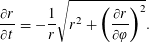 $$\begin{eqnarray}\frac{\unicode[STIX]{x2202}r}{\unicode[STIX]{x2202}t}=-\frac{1}{r}\sqrt{r^{2}+(\frac{\unicode[STIX]{x2202}r}{\unicode[STIX]{x2202}\unicode[STIX]{x1D711}}\biggr)^{2}}.\end{eqnarray}$$
The Eikonal equation has broad applications, ranging from geometric optics to abrasion. Two possible geometric interpretations of (1) appear in the literature (see [Reference Arnold1, Theorem 1], and [Reference Bloore2]), depending on which application is targeted by the model. We describe these interpretations below and illustrate them in Figure 1.
In the Eikonal wavefront model, starting with the boundary of a convex body
 $K(0)$
, one obtains the evolving hypersurface at time
$K(0)$
, one obtains the evolving hypersurface at time
 $t$
by translating every point of its boundary in the direction of the inward surface normal by a vector of length
$t$
by translating every point of its boundary in the direction of the inward surface normal by a vector of length
 $t$
(cf. Figure 1(a)). If
$t$
(cf. Figure 1(a)). If
 $K(0)$
is a smooth, convex body with minimal curvature radius
$K(0)$
is a smooth, convex body with minimal curvature radius
 $r_{\min }(0)$
(i.e. the reciprocal of the maximal principal curvature) then in the Eikonal wavefront model the evolving hypersurface will exhibit its first singularity at
$r_{\min }(0)$
(i.e. the reciprocal of the maximal principal curvature) then in the Eikonal wavefront model the evolving hypersurface will exhibit its first singularity at
 $t=r_{\min }(0)$
and for
$t=r_{\min }(0)$
and for
 $t>r_{\min }(0)$
it will develop self-intersecting, non-convex parts.
$t>r_{\min }(0)$
it will develop self-intersecting, non-convex parts.
In the Eikonal abrasion model, starting with the boundary of a convex body
 $K(0)$
, one obtains the evolving hypersurface at time
$K(0)$
, one obtains the evolving hypersurface at time
 $t$
by translating the supporting half space at every point of its boundary in the direction of the inward surface normal by a vector of length
$t$
by translating the supporting half space at every point of its boundary in the direction of the inward surface normal by a vector of length
 $t$
(cf. Figure 1(b)). Obviously, in this model the evolving hypersurface
$t$
(cf. Figure 1(b)). Obviously, in this model the evolving hypersurface
 $K(t)$
will remain convex; however, initially smooth shapes will also develop singularities. The first such singularity appears, similarly to the wavefront model, at
$K(t)$
will remain convex; however, initially smooth shapes will also develop singularities. The first such singularity appears, similarly to the wavefront model, at
 $t=r_{\min }(0)$
. The singularities of the evolving hypersurface in the Eikonal abrasion model correspond to the self-intersections in the Eikonal wavefront model.
$t=r_{\min }(0)$
. The singularities of the evolving hypersurface in the Eikonal abrasion model correspond to the self-intersections in the Eikonal wavefront model.

Figure 1 Alternative interpretations of the Eikonal equation (1): (a) The Eikonal wavefront model and (b) the Eikonal abrasion model.
The current paper focuses on the Eikonal abrasion model (for details about global geometrical evolution in the wavefront model see, for example, [Reference Knill19]). In an abrasion process an abrading object
 $K$
with surface area
$K$
with surface area
 $A(K)$
is bombarded by abraders
$A(K)$
is bombarded by abraders
 $k$
with surface area
$k$
with surface area
 $A(k)$
arriving from directions uniformly distributed over the sphere and the surface ratio
$A(k)$
arriving from directions uniformly distributed over the sphere and the surface ratio
 $\unicode[STIX]{x1D707}=A(k)/A(K)$
is a characteristic parameter of the process [Reference Bloore2]. In this context, the Eikonal equation has been introduced by Bloore [Reference Bloore2] as a model for the limit
$\unicode[STIX]{x1D707}=A(k)/A(K)$
is a characteristic parameter of the process [Reference Bloore2]. In this context, the Eikonal equation has been introduced by Bloore [Reference Bloore2] as a model for the limit
 $\unicode[STIX]{x1D707}\rightarrow 0$
. This model can explain, among other things, the shapes of desert rocks abraded by wind-blown sand [Reference Várkonyi, Laity and Domokos28] and also the shapes of asteroids [Reference Domokos, Sipos, Szabó and Várkonyi8], which evolve under many small impacts from micrometeorites. In the latter application a geometric feature of the Eikonal model played a key role: it has been observed [Reference Domokos, Sipos, Várkonyi and Szabó10] that evolution under the Eikonal abrasion model decreases the roundedness (i.e. increases the thinness/flatness) of a shape. This observation offered so far the only natural explanation for the grossly elongated shape of the first observed interstellar asteroid ‘Oumuamua [Reference Domokos, Sipos, Várkonyi and Szabó10]. The aim of the present note is to give a mathematical verification of this observation. We prove that in this model the isoperimetric quotient, which is one of the most broadly used measures of resemblance to a sphere, decreases as a function of time. There has been great interest in proving the monotonicity of the isoperimetric quotient and related quantities under geometric evolution equations, most notably, curvature-driven evolution equations [Reference Gage13, Reference Hamilton16, Reference Huisken17]. Even though the Eikonal equation (1) is fairly different from these flows, the evolution of the isoperimetric quotient under (1) still looks like an attractive problem: as we will point out in §3.2, in mathematical models of abrasion the Eikonal model is coupled with curvature-driven terms.
$\unicode[STIX]{x1D707}\rightarrow 0$
. This model can explain, among other things, the shapes of desert rocks abraded by wind-blown sand [Reference Várkonyi, Laity and Domokos28] and also the shapes of asteroids [Reference Domokos, Sipos, Szabó and Várkonyi8], which evolve under many small impacts from micrometeorites. In the latter application a geometric feature of the Eikonal model played a key role: it has been observed [Reference Domokos, Sipos, Várkonyi and Szabó10] that evolution under the Eikonal abrasion model decreases the roundedness (i.e. increases the thinness/flatness) of a shape. This observation offered so far the only natural explanation for the grossly elongated shape of the first observed interstellar asteroid ‘Oumuamua [Reference Domokos, Sipos, Várkonyi and Szabó10]. The aim of the present note is to give a mathematical verification of this observation. We prove that in this model the isoperimetric quotient, which is one of the most broadly used measures of resemblance to a sphere, decreases as a function of time. There has been great interest in proving the monotonicity of the isoperimetric quotient and related quantities under geometric evolution equations, most notably, curvature-driven evolution equations [Reference Gage13, Reference Hamilton16, Reference Huisken17]. Even though the Eikonal equation (1) is fairly different from these flows, the evolution of the isoperimetric quotient under (1) still looks like an attractive problem: as we will point out in §3.2, in mathematical models of abrasion the Eikonal model is coupled with curvature-driven terms.
In order to formulate our main result, we introduce some notation for the concepts described above. First, by
 $\mathbf{B}^{d}$
we denote the closed unit ball with the origin
$\mathbf{B}^{d}$
we denote the closed unit ball with the origin
 $o$
as its center, and set
$o$
as its center, and set
 $\mathbb{S}^{d-1}=\operatorname{bd}\mathbf{B}^{d}$
. Let
$\mathbb{S}^{d-1}=\operatorname{bd}\mathbf{B}^{d}$
. Let
 $K$
be a convex body in
$K$
be a convex body in
 $\mathbb{R}^{d}$
; that is, a compact, convex set with non-empty interior. Recall that the support function
$\mathbb{R}^{d}$
; that is, a compact, convex set with non-empty interior. Recall that the support function
 $h_{K}:\mathbb{S}^{d-1}\rightarrow \mathbb{R}$
of
$h_{K}:\mathbb{S}^{d-1}\rightarrow \mathbb{R}$
of
 $K$
is defined by
$K$
is defined by
 $h_{K}(u)=\sup \{\langle u,p\rangle :p\in K\}$
for all
$h_{K}(u)=\sup \{\langle u,p\rangle :p\in K\}$
for all
 $u\in \mathbb{S}^{d-1}$
[Reference Schneider26]. For any
$u\in \mathbb{S}^{d-1}$
[Reference Schneider26]. For any
 $t\geqslant 0$
, we let
$t\geqslant 0$
, we let
 $H_{K}(u,t)$
be the closed half space defined by
$H_{K}(u,t)$
be the closed half space defined by
 $\{x\in \mathbb{R}^{d}:\langle x,u\rangle \leqslant h_{K}(u)-t\}$
. Note that for any
$\{x\in \mathbb{R}^{d}:\langle x,u\rangle \leqslant h_{K}(u)-t\}$
. Note that for any
 $t>0$
, we have that
$t>0$
, we have that
 $K(t)=\bigcap _{u\in S^{d-1}}H_{K}(u,t)$
. Observe that if
$K(t)=\bigcap _{u\in S^{d-1}}H_{K}(u,t)$
. Observe that if
 $r(K)$
is the radius of a largest ball contained in
$r(K)$
is the radius of a largest ball contained in
 $K$
, then for any
$K$
, then for any
 $0\leqslant t<r(K)~K(t)$
is a convex body, for
$0\leqslant t<r(K)~K(t)$
is a convex body, for
 $t=r(K)$
,
$t=r(K)$
,
 $K(t)$
is a compact, convex set with no interior point, and for
$K(t)$
is a compact, convex set with no interior point, and for
 $t>r(K)$
,
$t>r(K)$
,
 $K(t)=\emptyset$
. Following [Reference Pisanski, Kaufman, Bokal, Kirby and Graovac25], we define the isoperimetric quotient of any convex body
$K(t)=\emptyset$
. Following [Reference Pisanski, Kaufman, Bokal, Kirby and Graovac25], we define the isoperimetric quotient of any convex body
 $M$
as
$M$
as
 $I(M)=V(M)/(A(M))^{d/(d-1)}$
where
$I(M)=V(M)/(A(M))^{d/(d-1)}$
where
 $V(\cdot )$
and
$V(\cdot )$
and
 $A(\cdot )$
denotes
$A(\cdot )$
denotes
 $d$
-dimensional volume and
$d$
-dimensional volume and
 $(d-1)$
-dimensional surface area, respectively. Our main result is as follows.
$(d-1)$
-dimensional surface area, respectively. Our main result is as follows.
Theorem 1. For any convex body
 $K$
, either
$K$
, either
 $I(K(t))$
is strictly decreasing on
$I(K(t))$
is strictly decreasing on
 $[0,r(K))$
, or there is some value
$[0,r(K))$
, or there is some value
 $t^{\star }\in [0,r(K))$
such that
$t^{\star }\in [0,r(K))$
such that
 $I(K(t))$
is strictly decreasing on
$I(K(t))$
is strictly decreasing on
 $[0,t^{\star }]$
and is a constant on
$[0,t^{\star }]$
and is a constant on
 $[t^{\star },r(K))$
. Furthermore, in the latter case, for any
$[t^{\star },r(K))$
. Furthermore, in the latter case, for any
 $t>t^{\star }$
,
$t>t^{\star }$
,
 $K(t)$
is homothetic to
$K(t)$
is homothetic to
 $K(t^{\star })$
.
$K(t^{\star })$
.
While our result highlights a fundamental property of the nonlinear PDE (1), our proof will rely entirely on ideas and concepts from convex geometry. In particular, as one can see in §2, the examined problem, and also the applied tools, are closely related to those used in [Reference Larson21], where, by an elegant method, the author gave a sharp lower estimate on the surface area of an inner parallel body of a convex body. These bodies also play a central role in the current paper: equation (1) can be regarded as a map from a convex body to one of its inner parallel bodies where time plays the role of the distance of this body from the original one. In this paper we study geometric properties of this map. The proof relies on an extensive use of mixed volumes and inequalities related to them. For the definitions and descriptions of these tools, the reader is referred to the books [Reference Gruber15, Reference Schneider26] or the paper [Reference Larson21]. Some elements of our proof can also be found in [Reference Schneider26, §7.2] and in [Reference Stachó27].
2 Proof of Theorem 1
During the proof, for any convex body
 $M$
and boundary point
$M$
and boundary point
 $p\in \operatorname{bd}M$
we denote the set of outer unit normal vectors of
$p\in \operatorname{bd}M$
we denote the set of outer unit normal vectors of
 $M$
at
$M$
at
 $p$
by
$p$
by
 $N_{p}(M)\subseteq \mathbb{S}^{d-1}$
. Note that this set is a spherically convex, compact set, and hence, in particular, it is contained in an open hemisphere of
$N_{p}(M)\subseteq \mathbb{S}^{d-1}$
. Note that this set is a spherically convex, compact set, and hence, in particular, it is contained in an open hemisphere of
 $\mathbb{S}^{d-1}$
. The set of smooth (or regular) points of
$\mathbb{S}^{d-1}$
. The set of smooth (or regular) points of
 $M$
(i.e. the set of boundary points
$M$
(i.e. the set of boundary points
 $p$
of
$p$
of
 $M$
such that
$M$
such that
 $N_{p}(M)$
is a singleton) is denoted by
$N_{p}(M)$
is a singleton) is denoted by
 $R(M)$
. Finally, we set
$R(M)$
. Finally, we set
 $N(M)=\bigcup _{p\in R(M)}N_{p}(M)$
, and
$N(M)=\bigcup _{p\in R(M)}N_{p}(M)$
, and
 $$\begin{eqnarray}F(M)=\{x\in \mathbb{R}^{d}:\langle x,u\rangle \leqslant 1~\text{for every}~u\in N(M)\}.\end{eqnarray}$$
This set is called the form body of
 $M$
(cf. [Reference Larson21] and [Reference Schneider26]), where the fact that it is indeed a convex body is an easy consequence of Alexandrov’s theorem (cf. [Reference Gruber15, Theorem 5.4]), stating that
$M$
(cf. [Reference Larson21] and [Reference Schneider26]), where the fact that it is indeed a convex body is an easy consequence of Alexandrov’s theorem (cf. [Reference Gruber15, Theorem 5.4]), stating that
 $\operatorname{bd}M$
is smooth (twice differentiable) at almost every point.
$\operatorname{bd}M$
is smooth (twice differentiable) at almost every point.
Now we prove Theorem 1. As volume and surface area are continuous with respect to Hausdorff distance and are strictly increasing with respect to containment in the family of convex bodies, both
 $V(K(t))$
and
$V(K(t))$
and
 $A(K(t))$
are positive continuous, strictly decreasing functions of
$A(K(t))$
are positive continuous, strictly decreasing functions of
 $t$
on the interval
$t$
on the interval
 $[0,r(K))$
. This implies that
$[0,r(K))$
. This implies that
 $I(K(t))$
is also continuous on this interval.
$I(K(t))$
is also continuous on this interval.
Consider some
 $0<t_{0}<r(K)$
. For brevity, we set
$0<t_{0}<r(K)$
. For brevity, we set
 $K(t_{0})=K_{0}$
,
$K(t_{0})=K_{0}$
,
 $N(K(t_{0}))=N_{0}$
,
$N(K(t_{0}))=N_{0}$
,
 $F(K(t_{0}))=F_{0}$
and
$F(K(t_{0}))=F_{0}$
and
 $I(K(t))=I(t)$
. Let
$I(K(t))=I(t)$
. Let
 $p\in \operatorname{bd}K_{0}$
. By the definition of
$p\in \operatorname{bd}K_{0}$
. By the definition of
 $K(t)$
, for any
$K(t)$
, for any
 $0\leqslant t\leqslant t_{0}$
the minimum of the distances of
$0\leqslant t\leqslant t_{0}$
the minimum of the distances of
 $p$
from the supporting hyperplanes of
$p$
from the supporting hyperplanes of
 $\operatorname{bd}K(t)$
is equal to
$\operatorname{bd}K(t)$
is equal to
 $t_{0}-t$
. Since this minimum is attained at some point
$t_{0}-t$
. Since this minimum is attained at some point
 $q\in \operatorname{bd}K(t)$
, the ball
$q\in \operatorname{bd}K(t)$
, the ball
 $p+(t-t_{0})\mathbf{B}^{d}$
touches
$p+(t-t_{0})\mathbf{B}^{d}$
touches
 $\operatorname{bd}K(t)$
from inside. Thus,
$\operatorname{bd}K(t)$
from inside. Thus,
 $K_{0}+(t_{0}-t)\mathbf{B}^{d}\subseteq K(t)$
. On the other hand, we also have
$K_{0}+(t_{0}-t)\mathbf{B}^{d}\subseteq K(t)$
. On the other hand, we also have
 $h_{K(t)}(u)=h_{K_{0}}(u)+(t_{0}-t)$
for any
$h_{K(t)}(u)=h_{K_{0}}(u)+(t_{0}-t)$
for any
 $u\in N_{0}$
, which yields that
$u\in N_{0}$
, which yields that
 $K(t)\subseteq K_{0}+(t_{0}-t)F_{0}$
. We remark that the geometric arguments leading to these two containment relations can be found in a comprehensive form in [Reference Larson21]. We note that if
$K(t)\subseteq K_{0}+(t_{0}-t)F_{0}$
. We remark that the geometric arguments leading to these two containment relations can be found in a comprehensive form in [Reference Larson21]. We note that if
 $K_{0}$
is smooth, then so is
$K_{0}$
is smooth, then so is
 $K(t)$
for every
$K(t)$
for every
 $0\leqslant t\leqslant t_{0}$
, implying that
$0\leqslant t\leqslant t_{0}$
, implying that
 $K(t)=K_{0}+(t_{0}-t)\mathbf{B}^{d}$
in this case. More generally,
$K(t)=K_{0}+(t_{0}-t)\mathbf{B}^{d}$
in this case. More generally,
 $N(K(t))$
decreases and
$N(K(t))$
decreases and
 $F(K(t))$
increases in time with respect to containment; that is, for any
$F(K(t))$
increases in time with respect to containment; that is, for any
 $0\leqslant t_{1}<t_{2}<r(K)$
we have
$0\leqslant t_{1}<t_{2}<r(K)$
we have
 $N(K(t_{2}))\subseteq N(K(t_{1}))$
and
$N(K(t_{2}))\subseteq N(K(t_{1}))$
and
 $F(K(t_{1}))\subseteq F(K(t_{2}))$
.
$F(K(t_{1}))\subseteq F(K(t_{2}))$
.
Set
 $L(t)=K_{0}+(t_{0}-t)\mathbf{B}^{d}$
, and
$L(t)=K_{0}+(t_{0}-t)\mathbf{B}^{d}$
, and
 $M(t)=K_{0}+(t_{0}-t)F_{0}$
. By Minkowski’s theorem on mixed volumes [Reference Schneider26], we have
$M(t)=K_{0}+(t_{0}-t)F_{0}$
. By Minkowski’s theorem on mixed volumes [Reference Schneider26], we have
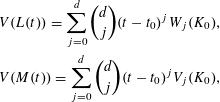 $$\begin{eqnarray}\begin{array}{@{}l@{}}\displaystyle V(L(t))=\mathop{\sum }_{j=0}^{d}\binom{d}{j}(t-t_{0})^{j}W_{j}(K_{0}),\\ \displaystyle V(M(t))=\mathop{\sum }_{j=0}^{d}\binom{d}{j}(t-t_{0})^{j}V_{j}(K_{0}),\end{array}\end{eqnarray}$$
where
 $W_{j}(K_{0})$
is the
$W_{j}(K_{0})$
is the
 $j$
th quermassintegral of
$j$
th quermassintegral of
 $K_{0}$
, and we denote the mixed volume
$K_{0}$
, and we denote the mixed volume
 $$\begin{eqnarray}V(\overbrace{K_{0},\ldots ,K_{0}}^{d-j},\overbrace{F_{0},\ldots ,F_{0}}^{j})\end{eqnarray}$$
by
 $V_{j}(K_{0})$
.
$V_{j}(K_{0})$
.
Observe that
 $W_{0}(K_{0})=V_{0}(K_{0})=V(K_{0})$
, and that
$W_{0}(K_{0})=V_{0}(K_{0})=V(K_{0})$
, and that
 $dW_{1}(K_{0})=A(K_{0})$
. We show that
$dW_{1}(K_{0})=A(K_{0})$
. We show that
 $dV_{1}(K_{0})=A(K_{0})$
as well. Since both mixed volumes and surface area are continuous with respect to Hausdorff distance, it suffices to prove this equality for polytopes, and thus, assume for the moment that
$dV_{1}(K_{0})=A(K_{0})$
as well. Since both mixed volumes and surface area are continuous with respect to Hausdorff distance, it suffices to prove this equality for polytopes, and thus, assume for the moment that
 $K_{0}$
is a polytope. In this case
$K_{0}$
is a polytope. In this case
 $F_{0}$
is the polytope, circumscribed about
$F_{0}$
is the polytope, circumscribed about
 $\mathbf{B}^{d}$
, whose outer unit facet normal vectors coincide with those of
$\mathbf{B}^{d}$
, whose outer unit facet normal vectors coincide with those of
 $K_{0}$
. Thus,
$K_{0}$
. Thus,
 $M(t)$
can be decomposed into
$M(t)$
can be decomposed into
 $K_{0}$
, cylinders of height
$K_{0}$
, cylinders of height
 $t_{0}-t$
with the facets of
$t_{0}-t$
with the facets of
 $K_{0}$
as bases, and sets in the
$K_{0}$
as bases, and sets in the
 $\unicode[STIX]{x1D70C}(t_{0}-t)$
-neighborhood of the
$\unicode[STIX]{x1D70C}(t_{0}-t)$
-neighborhood of the
 $(d-2)$
-faces of
$(d-2)$
-faces of
 $K(t_{0})$
, where
$K(t_{0})$
, where
 $\unicode[STIX]{x1D70C}=\operatorname{diam}F_{0}$
. The volume of this set is
$\unicode[STIX]{x1D70C}=\operatorname{diam}F_{0}$
. The volume of this set is
 $$\begin{eqnarray}V(M(t))=V(K_{0})+(t_{0}-t)A(K_{0})+O((t_{0}-t)^{2}),\end{eqnarray}$$
implying
 $-dV_{1}(K_{0})=(d/dt)V(M(t))|_{t=t_{0}}=-A(K(t_{0}))$
.
$-dV_{1}(K_{0})=(d/dt)V(M(t))|_{t=t_{0}}=-A(K(t_{0}))$
.
Let us define the quantity
 $$\begin{eqnarray}\text{}\underline{I}(t)=\frac{V(L(t))}{A(M(t))^{d/(d-1)}}.\end{eqnarray}$$
We note that
 $\text{}\underline{I}(t)$
depends on
$\text{}\underline{I}(t)$
depends on
 $t_{0}$
and it is defined only for
$t_{0}$
and it is defined only for
 $0\leqslant t\leqslant t_{0}$
. Furthermore, as both volume and surface area are strictly increasing with respect to inclusion, we have
$0\leqslant t\leqslant t_{0}$
. Furthermore, as both volume and surface area are strictly increasing with respect to inclusion, we have
 $\text{}\underline{I}(t)\leqslant I(t)$
. Differentiating this quantity, the formulas in (4) and their connection with
$\text{}\underline{I}(t)\leqslant I(t)$
. Differentiating this quantity, the formulas in (4) and their connection with
 $A(K_{0})$
yields that
$A(K_{0})$
yields that
 $$\begin{eqnarray}\text{}\underline{I}_{-}^{\prime }(t_{0})=-\frac{d^{2}}{A(K_{0})^{(2d-1)/(d-1)}}(V_{1}(K_{0})^{2}-V_{0}(K_{0})V_{2}(K_{0})),\end{eqnarray}$$
which is not positive by the second inequality of Minkowski [Reference Gruber15].
We show that if
 $\text{}\underline{I}_{-}^{\prime }(t_{0})=0$
, then
$\text{}\underline{I}_{-}^{\prime }(t_{0})=0$
, then
 $K_{0}$
is homothetic to
$K_{0}$
is homothetic to
 $F_{0}$
. By [Reference Schneider26, Theorem 7.6.19], since both
$F_{0}$
. By [Reference Schneider26, Theorem 7.6.19], since both
 $K_{0}$
and
$K_{0}$
and
 $F_{0}$
are
$F_{0}$
are
 $d$
-dimensional,
$d$
-dimensional,
 $(V_{1}(K_{0}))^{2}=V_{0}(K_{0})V_{2}(K_{0})$
implies that
$(V_{1}(K_{0}))^{2}=V_{0}(K_{0})V_{2}(K_{0})$
implies that
 $K_{0}$
is homothetic to a
$K_{0}$
is homothetic to a
 $(d-2)$
-tangential body of
$(d-2)$
-tangential body of
 $F_{0}$
. More specifically,
$F_{0}$
. More specifically,
 $K_{0}$
has a homothetic copy
$K_{0}$
has a homothetic copy
 $K^{\prime }$
such that
$K^{\prime }$
such that
 $F_{0}\subseteq K^{\prime }$
, and every supporting hyperplane of
$F_{0}\subseteq K^{\prime }$
, and every supporting hyperplane of
 $K^{\prime }$
that does not support
$K^{\prime }$
that does not support
 $F_{0}$
contains only
$F_{0}$
contains only
 $(d-3)$
-singular (cf. [Reference Schneider26, §2.2]) or, in particular, singular points of
$(d-3)$
-singular (cf. [Reference Schneider26, §2.2]) or, in particular, singular points of
 $K^{\prime }$
. Hence, every supporting hyperplane of
$K^{\prime }$
. Hence, every supporting hyperplane of
 $K^{\prime }$
that contains a smooth point of
$K^{\prime }$
that contains a smooth point of
 $\operatorname{bd}K^{\prime }$
supports
$\operatorname{bd}K^{\prime }$
supports
 $F_{0}$
as well. Thus, the definition of
$F_{0}$
as well. Thus, the definition of
 $F_{0}$
and the relation
$F_{0}$
and the relation
 $F_{0}\subseteq K^{\prime }$
yields
$F_{0}\subseteq K^{\prime }$
yields
 $F_{0}=K^{\prime }$
. This means that if
$F_{0}=K^{\prime }$
. This means that if
 $\text{}\underline{I}_{-}^{\prime }(t_{0})=0$
, then
$\text{}\underline{I}_{-}^{\prime }(t_{0})=0$
, then
 $F_{0}$
is homothetic to
$F_{0}$
is homothetic to
 $K_{0}$
. Note that the reversed statement also holds: if
$K_{0}$
. Note that the reversed statement also holds: if
 $F_{0}$
is homothetic to
$F_{0}$
is homothetic to
 $K_{0}$
, then
$K_{0}$
, then
 $\text{}\underline{I}_{-}^{\prime }(t_{0})=0$
, and, even more, in this case
$\text{}\underline{I}_{-}^{\prime }(t_{0})=0$
, and, even more, in this case
 $K(t)$
is homothetic to
$K(t)$
is homothetic to
 $K_{0}$
for any
$K_{0}$
for any
 $t>t_{0}$
.
$t>t_{0}$
.
Let
 $t^{\star }$
denote the smallest value of
$t^{\star }$
denote the smallest value of
 $t$
such that
$t$
such that
 $\text{}\underline{I}_{-}^{\prime }(t)=0$
. Then
$\text{}\underline{I}_{-}^{\prime }(t)=0$
. Then
 $K(t)$
is homothetic to
$K(t)$
is homothetic to
 $K(t^{\star })$
for any
$K(t^{\star })$
for any
 $t\in [t^{\star },r(K))$
, and
$t\in [t^{\star },r(K))$
, and
 $I(t)$
is a constant on this interval. To finish the proof we need to show that
$I(t)$
is a constant on this interval. To finish the proof we need to show that
 $I(t)$
strictly decreases on
$I(t)$
strictly decreases on
 $[0,t^{\star }]$
.
$[0,t^{\star }]$
.
Since
 $\text{}\underline{I}_{-}^{\prime }(t_{0})<0$
for any
$\text{}\underline{I}_{-}^{\prime }(t_{0})<0$
for any
 $0<t_{0}<t^{\star }$
, for any such
$0<t_{0}<t^{\star }$
, for any such
 $t_{0}$
there is some
$t_{0}$
there is some
 $\unicode[STIX]{x1D700}=\unicode[STIX]{x1D700}(K,t_{0})>0$
such that
$\unicode[STIX]{x1D700}=\unicode[STIX]{x1D700}(K,t_{0})>0$
such that
 $I(t)\geqslant \text{}\underline{I}(t)>I(t_{0})$
for all
$I(t)\geqslant \text{}\underline{I}(t)>I(t_{0})$
for all
 $t\in (t_{0}-\unicode[STIX]{x1D700},t_{0})$
; that is, the function
$t\in (t_{0}-\unicode[STIX]{x1D700},t_{0})$
; that is, the function
 $I(t)$
is locally strictly decreasing from the left at every point. This and the continuity of
$I(t)$
is locally strictly decreasing from the left at every point. This and the continuity of
 $I(t)$
implies that
$I(t)$
implies that
 $I(t)$
strictly decreases on this interval. Indeed, suppose for contradiction that for some
$I(t)$
strictly decreases on this interval. Indeed, suppose for contradiction that for some
 $t_{1}<t_{2}$
we have
$t_{1}<t_{2}$
we have
 $I(t_{1})\leqslant I(t_{2})$
. By continuity,
$I(t_{1})\leqslant I(t_{2})$
. By continuity,
 $I(t)$
attains its global maximum on
$I(t)$
attains its global maximum on
 $[t_{1},t_{2}]$
at some
$[t_{1},t_{2}]$
at some
 $t^{\prime }\in [t_{1},t_{2}]$
. Clearly, since
$t^{\prime }\in [t_{1},t_{2}]$
. Clearly, since
 $I(t)$
is locally strictly decreasing from the left at
$I(t)$
is locally strictly decreasing from the left at
 $t^{\prime }$
it follows that
$t^{\prime }$
it follows that
 $t^{\prime }=t_{1}$
and
$t^{\prime }=t_{1}$
and
 $I(t_{1})>I(t_{2})$
, which contradicts the supposition.◻
$I(t_{1})>I(t_{2})$
, which contradicts the supposition.◻
3 Discussion
In this section we will point out connections to related results in convex geometry and also put our result in a broader setting to show that it may have implications beyond the specific PDE (1).
3.1 Connection to Lindelöf’s theorem and another type of asphericity
While our paper is primarily aimed to prove properties of the Eikonal abrasion model (1), the proof of Theorem 1 also implies a modest improvement of Lindelöf’s Theorem [Reference Lindelöf22]. Let
 $K$
be a convex
$K$
be a convex
 $d$
-polytope with outer unit normal vectors
$d$
-polytope with outer unit normal vectors
 $u_{1},u_{2},\ldots ,u_{n}$
of its facets. Then
$u_{1},u_{2},\ldots ,u_{n}$
of its facets. Then
 $F(K)$
is the polytope with the same vectors as outer facet unit normal vectors, circumscribed about the unit ball
$F(K)$
is the polytope with the same vectors as outer facet unit normal vectors, circumscribed about the unit ball
 $\mathbf{B}^{d}$
. For this case, Theorem 1 states that
$\mathbf{B}^{d}$
. For this case, Theorem 1 states that
 $I(K+tF(K))$
with
$I(K+tF(K))$
with
 $t\in [0,\infty )$
(or, since homothety does not change the isoperimetric ratio,
$t\in [0,\infty )$
(or, since homothety does not change the isoperimetric ratio,
 $((1-t)K+tF(K))$
with
$((1-t)K+tF(K))$
with
 $t\in [0,1]$
), is a strictly increasing function of
$t\in [0,1]$
), is a strictly increasing function of
 $t$
, unless
$t$
, unless
 $K$
is homothetic to
$K$
is homothetic to
 $F(K)$
. This special case is a stronger form of Lindelöf’s theorem [Reference Lindelöf22] stating that among convex polytopes with given outer facet unit normal vectors, those circumscribed about a ball has maximal isoperimetric ratio.
$F(K)$
. This special case is a stronger form of Lindelöf’s theorem [Reference Lindelöf22] stating that among convex polytopes with given outer facet unit normal vectors, those circumscribed about a ball has maximal isoperimetric ratio.
This connection leads us to the following definition.
Definition 1. Let
 $K$
be a convex body. Let the convex body
$K$
be a convex body. Let the convex body
 $E(K)$
be the intersection of the closed supporting half spaces whose boundary touches each largest inscribed ball of
$E(K)$
be the intersection of the closed supporting half spaces whose boundary touches each largest inscribed ball of
 $K$
. We call this closed, convex set the envelope of
$K$
. We call this closed, convex set the envelope of
 $K$
under equation (1), or shortly, the envelope of
$K$
under equation (1), or shortly, the envelope of
 $K$
.
$K$
.
We remark that
 $F(K)$
is contained in a translate of
$F(K)$
is contained in a translate of
 $(1/r(K))E(K)$
, and that the quantity
$(1/r(K))E(K)$
, and that the quantity
 $t^{\star }$
appearing in Theorem 1 has the property that this is the smallest value of
$t^{\star }$
appearing in Theorem 1 has the property that this is the smallest value of
 $t$
such that this containment is not strict. In the spirit of [Reference Dudov and Meshcheryakova11], we will use the following.
$t$
such that this containment is not strict. In the spirit of [Reference Dudov and Meshcheryakova11], we will use the following.
Definition 2. Let
 $K$
be a convex body and let
$K$
be a convex body and let
 $r(K)$
and
$r(K)$
and
 $R(K)$
denote the radius of a largest inscribed and the smallest circumscribed sphere of
$R(K)$
denote the radius of a largest inscribed and the smallest circumscribed sphere of
 $K$
, respectively. Then the asphericity of
$K$
, respectively. Then the asphericity of
 $K$
is given by
$K$
is given by
 $\unicode[STIX]{x1D6FC}(K)=R(K)/r(K)$
.
$\unicode[STIX]{x1D6FC}(K)=R(K)/r(K)$
.
Proposition 1. Under the Eikonal abrasion model given by equation (1), acting on the convex body
 $K(t)$
,
$K(t)$
,
 $\unicode[STIX]{x1D6FC}(K(t))$
is an increasing function of
$\unicode[STIX]{x1D6FC}(K(t))$
is an increasing function of
 $t$
on
$t$
on
 $[0,r(K))$
.
$[0,r(K))$
.
Proof. Recall the definition of
 $K(t)$
in the Introduction:
$K(t)$
in the Introduction:
 $$\begin{eqnarray}K(t)=\mathop{\bigcap }_{u\in S^{d-1}}H_{K}(u,t),\end{eqnarray}$$
where
 $H_{K}(u,t)$
is the closed half space defined by
$H_{K}(u,t)$
is the closed half space defined by
 $\{x\in \mathbb{R}^{d}:\langle x,u\rangle \leqslant h_{K}(u)-t\}$
. Since changing the origin only translates
$\{x\in \mathbb{R}^{d}:\langle x,u\rangle \leqslant h_{K}(u)-t\}$
. Since changing the origin only translates
 $K(t)$
, we may assume that
$K(t)$
, we may assume that
 $o$
is the center of a largest inscribed ball in
$o$
is the center of a largest inscribed ball in
 $K$
. Then
$K$
. Then
 $r(K)=\min _{u\in S^{d-1}}h_{K}(u)$
, and it is easy to see (for a formal proof, see [Reference Larson21, Lemma 1.4]) that
$r(K)=\min _{u\in S^{d-1}}h_{K}(u)$
, and it is easy to see (for a formal proof, see [Reference Larson21, Lemma 1.4]) that
 $r(K(t))=r(K)-t$
for all values
$r(K(t))=r(K)-t$
for all values
 $t\in [0,r(K))$
.
$t\in [0,r(K))$
.
Note that for any
 $t\in [0,r(K))$
, the radius of a largest inscribed ball of
$t\in [0,r(K))$
, the radius of a largest inscribed ball of
 $(r(K)/r(K(t)))K(t)$
is
$(r(K)/r(K(t)))K(t)$
is
 $r(K)$
. On the other hand, for any
$r(K)$
. On the other hand, for any
 $u\in \mathbb{S}^{d-1}$
, the inequality
$u\in \mathbb{S}^{d-1}$
, the inequality
 $0<r(K)\leqslant h_{K}(u)$
yields that
$0<r(K)\leqslant h_{K}(u)$
yields that
 $h_{K}(u)/r(K)\leqslant (h_{K}(u)-t)/(r(K)-t)$
for all
$h_{K}(u)/r(K)\leqslant (h_{K}(u)-t)/(r(K)-t)$
for all
 $0<t<r(K)$
, implying that
$0<t<r(K)$
, implying that
 $K\subseteq (r(K)/r(K(t)))K(t)$
. Thus,
$K\subseteq (r(K)/r(K(t)))K(t)$
. Thus,
 $\unicode[STIX]{x1D6FC}(K)\leqslant \unicode[STIX]{x1D6FC}(K(t))$
for every value of
$\unicode[STIX]{x1D6FC}(K)\leqslant \unicode[STIX]{x1D6FC}(K(t))$
for every value of
 $t$
. Since the same argument implies also that
$t$
. Since the same argument implies also that
 $K(t_{1})\subseteq K(t_{2})$
for all
$K(t_{1})\subseteq K(t_{2})$
for all
 $0\leqslant t_{1}\leqslant t_{2}<r(K)$
,
$0\leqslant t_{1}\leqslant t_{2}<r(K)$
,
 $\unicode[STIX]{x1D6FC}(K(t))$
is an increasing function of
$\unicode[STIX]{x1D6FC}(K(t))$
is an increasing function of
 $t$
.◻
$t$
.◻
Observe that the proof of Proposition 1 indicates that if
 $E(K)$
is bounded, then as
$E(K)$
is bounded, then as
 $t$
tends to
$t$
tends to
 $r(K)$
,
$r(K)$
,
 $K(t)$
“approaches”
$K(t)$
“approaches”
 $E(K)$
up to homothety. The proof also illustrates that the monotonicity of the asphericity given in Definition 2 is much easier to establish than the monotonicity of the isoperimetric quotient (which we did in Theorem 1). Nevertheless, as we will point out below, the latter result has broader consequences in abrasion models.
$E(K)$
up to homothety. The proof also illustrates that the monotonicity of the asphericity given in Definition 2 is much easier to establish than the monotonicity of the isoperimetric quotient (which we did in Theorem 1). Nevertheless, as we will point out below, the latter result has broader consequences in abrasion models.
3.2 Connection to other surface evolution models
As remarked in the introduction, the Eikonal model corresponds to the rather special limit
 $\unicode[STIX]{x1D707}\rightarrow 0$
in collisional abrasion when the relative size of the incoming abraders and the abraded object approaches zero. The other extreme limit is
$\unicode[STIX]{x1D707}\rightarrow 0$
in collisional abrasion when the relative size of the incoming abraders and the abraded object approaches zero. The other extreme limit is
 $\unicode[STIX]{x1D707}\rightarrow \infty$
, when the incoming particles are very large, in this case they can be modeled by hyperplanes. This case has been first treated in the classic paper by Firey [Reference Firey12], who arrived at the formula
$\unicode[STIX]{x1D707}\rightarrow \infty$
, when the incoming particles are very large, in this case they can be modeled by hyperplanes. This case has been first treated in the classic paper by Firey [Reference Firey12], who arrived at the formula
 $$\begin{eqnarray}v=c\unicode[STIX]{x1D705},\end{eqnarray}$$
where
 $\unicode[STIX]{x1D705}$
is the curvature at the boundary point of the abrading particle if (5) is interpreted in two dimensions, it is the Gaussian curvature in the three-dimensional case and
$\unicode[STIX]{x1D705}$
is the curvature at the boundary point of the abrading particle if (5) is interpreted in two dimensions, it is the Gaussian curvature in the three-dimensional case and
 $c$
is a scalar coefficient. The planar version of (5) is called the curve shortening flow, under which, by a result of Gage [Reference Gage13], isoperimetric quotient is monotonically increasing. Bloore [Reference Bloore2] generalized Firey’s model by admitting incoming particles with arbitrary size. Quite surprisingly, the PDE describing the general case turned out to be a linear combination of the two extreme scenarios. In two dimensions, Bloore’s equation is
$c$
is a scalar coefficient. The planar version of (5) is called the curve shortening flow, under which, by a result of Gage [Reference Gage13], isoperimetric quotient is monotonically increasing. Bloore [Reference Bloore2] generalized Firey’s model by admitting incoming particles with arbitrary size. Quite surprisingly, the PDE describing the general case turned out to be a linear combination of the two extreme scenarios. In two dimensions, Bloore’s equation is
 $$\begin{eqnarray}v=1+c\unicode[STIX]{x1D705},\end{eqnarray}$$
where
 $\unicode[STIX]{x1D705}$
is the curvature and
$\unicode[STIX]{x1D705}$
is the curvature and
 $c$
is the (normalized) perimeter of the incoming particles. Physical intuition suggests that in equation (6) the two additive terms represent geometrically opposite, competing effects; however, it is not easy to formalize this observation. Our Theorem 1, combined with Gage’s result [Reference Gage13] shows that as far as the evolution of the isoperimetric ratio is concerned, the two terms are indeed acting in opposite directions.
$c$
is the (normalized) perimeter of the incoming particles. Physical intuition suggests that in equation (6) the two additive terms represent geometrically opposite, competing effects; however, it is not easy to formalize this observation. Our Theorem 1, combined with Gage’s result [Reference Gage13] shows that as far as the evolution of the isoperimetric ratio is concerned, the two terms are indeed acting in opposite directions.
The Eikonal equation (1) can be also interpreted as a speed defined for the outward surface normal and this leads to the time-reversed Eikonal model where the wavefront and surface evolution interpretations do not need to be distinguished; however, the initial shape
 $K(0)$
has to be smooth, otherwise the flow is not unique. Unlike the inward flow, the outward Eikonal flow preserves the smoothness of shapes. It is easy to see that in the
$K(0)$
has to be smooth, otherwise the flow is not unique. Unlike the inward flow, the outward Eikonal flow preserves the smoothness of shapes. It is easy to see that in the
 $t\rightarrow \infty$
limit the outward flow converges to the sphere, and as a trivial consequence of Theorem 1 we can also see that
$t\rightarrow \infty$
limit the outward flow converges to the sphere, and as a trivial consequence of Theorem 1 we can also see that
 $I(t)$
is growing monotonically under this flow. The time-reversed Eikonal flow appears in one of the most broadly used surface growth equations in soft condensed matter physics, the Kardar–Parisi–Zhang (KPZ) equation [Reference Kardar, Paris and Zhang18]. The deterministic version of the KPZ equation can be written [Reference Marsilli, Maritan, Toigo and Banavar24, equation 29] in two dimensions as
$I(t)$
is growing monotonically under this flow. The time-reversed Eikonal flow appears in one of the most broadly used surface growth equations in soft condensed matter physics, the Kardar–Parisi–Zhang (KPZ) equation [Reference Kardar, Paris and Zhang18]. The deterministic version of the KPZ equation can be written [Reference Marsilli, Maritan, Toigo and Banavar24, equation 29] in two dimensions as
 $$\begin{eqnarray}v=-1+c\unicode[STIX]{x1D705},\end{eqnarray}$$
which is reminiscent of the Bloore flow (6); however, the additive terms have opposite sign, so physical intuition suggests that for any smooth, convex curve
 $K(0)$
evolving under (7) the isoperimetric quotient
$K(0)$
evolving under (7) the isoperimetric quotient
 $I(t)$
is a monotonically increasing function. We also remark that the Eikonal abrasion model appears to be the only one among collisional abrasion models where the isoperimetric ratio decreases. However, among models for frictional abrasion [Reference Domokos and Lángi7] one can find analogous evolutions.
$I(t)$
is a monotonically increasing function. We also remark that the Eikonal abrasion model appears to be the only one among collisional abrasion models where the isoperimetric ratio decreases. However, among models for frictional abrasion [Reference Domokos and Lángi7] one can find analogous evolutions.
3.3 Evolution of the number of critical points
One can obtain interesting information about geometric evolutions by identifying quantities which evolve monotonically under the flow. Such quantities may be either real-valued (prominent examples are versions of the isoperimetric quotient [Reference Gage13, Reference Hamilton16]), or alternatively, they may be integer-valued. Integer-valued quantities have been investigated mostly in connection of the heat equation and other flows related to image processing [Reference Koenderink20, Reference Lu, Cao and Mumford23] and a prominent example is the number
 $N(t)$
of critical points. Here the evolving hypersurface is defined by the scalar distance
$N(t)$
of critical points. Here the evolving hypersurface is defined by the scalar distance
 $r$
measured either from a hyperplane (in orthogonal coordinates) or from a fixed point (in polar coordinates, e.g. such as in equation (2)). These hypersurfaces correspond to graphs of real valued functions
$r$
measured either from a hyperplane (in orthogonal coordinates) or from a fixed point (in polar coordinates, e.g. such as in equation (2)). These hypersurfaces correspond to graphs of real valued functions
 $r$
defined on
$r$
defined on
 $\mathbb{R}^{d-1}$
or on
$\mathbb{R}^{d-1}$
or on
 $\mathbb{S}^{d-1}$
, respectively. Then the points satisfying
$\mathbb{S}^{d-1}$
, respectively. Then the points satisfying
 $\triangledown r=0$
are called critical. The function
$\triangledown r=0$
are called critical. The function
 $N(t)$
is constant for almost all values of
$N(t)$
is constant for almost all values of
 $t$
and we call it monotonic if it has jumps only in one direction. In the heat equation it was believed for an extended period of time that
$t$
and we call it monotonic if it has jumps only in one direction. In the heat equation it was believed for an extended period of time that
 $N(t)$
is decreasing monotonically; nevertheless, Damon [Reference Damon4] showed counterexamples. On the other hand, for the curve-shortening flow (5) Grayson [Reference Grayson14] proved that
$N(t)$
is decreasing monotonically; nevertheless, Damon [Reference Damon4] showed counterexamples. On the other hand, for the curve-shortening flow (5) Grayson [Reference Grayson14] proved that
 $N(t)$
is indeed decreasing monotonically. As illustrated in §3.2, the Eikonal abrasion model (1) is closely related to the curve shortening flow (5) via Bloore’s general abrasion model (6), so establishing a monotonicity result for
$N(t)$
is indeed decreasing monotonically. As illustrated in §3.2, the Eikonal abrasion model (1) is closely related to the curve shortening flow (5) via Bloore’s general abrasion model (6), so establishing a monotonicity result for
 $N(t)$
under (1) may help to clarify some aspects of shape evolution under (6). Unlike the heat equation and curvature-driven flows, in the Eikonal model the evolution of
$N(t)$
under (1) may help to clarify some aspects of shape evolution under (6). Unlike the heat equation and curvature-driven flows, in the Eikonal model the evolution of
 $N(t)$
is very easy to establish. Below we refer to the Eikonal equation written in polar coordinates for the distance function
$N(t)$
is very easy to establish. Below we refer to the Eikonal equation written in polar coordinates for the distance function
 $r$
, which, in two dimensions, is given in (2), or the geometric observations made in the paragraph before (4). We note that Proposition 2 has been proved under some smoothness condition in [Reference Domokos5, Lemma 2].
$r$
, which, in two dimensions, is given in (2), or the geometric observations made in the paragraph before (4). We note that Proposition 2 has been proved under some smoothness condition in [Reference Domokos5, Lemma 2].
Proposition 2. In the Eikonal wavefront model and in the time-reversed Eikonal model
 $N(t)$
is constant. In the Eikonal abrasion model
$N(t)$
is constant. In the Eikonal abrasion model
 $N(t)$
is decreasing monotonically.
$N(t)$
is decreasing monotonically.
Proof. The statement regarding the Eikonal wavefront model can be seen immediately as we realize that under (1), each point is moving along the associated inward surface normal. Points are critical if that normal passes through the reference point, so each point which is critical will remain critical and each point which is non-critical will remain non-critical under the flow (1). The same observation applies to the time-reversed Eikonal model. In the Eikonal wavefront model and in the time-reversed Eikonal model points travel on infinite (straight) trajectories, in the Eikonal abrasion model the straight trajectory is terminated after finite time. We know that the longest trajectories are of length
 $t=r(K)$
. In a non-degenerate case, that is, assuming that
$t=r(K)$
. In a non-degenerate case, that is, assuming that
 $K$
has finitely many critical points, there are finitely many trajectories we need to keep track of. Whenever a trajectory of a critical point terminates,
$K$
has finitely many critical points, there are finitely many trajectories we need to keep track of. Whenever a trajectory of a critical point terminates,
 $N(t)$
will decrease.◻
$N(t)$
will decrease.◻
Note that in the planar case, the first part of the statement also follows by the local analysis of codimension-one saddle-node bifurcations of critical points of
 $r(\unicode[STIX]{x1D711})$
evolving under (2). For details of this type of analysis see [Reference Domokos5].
$r(\unicode[STIX]{x1D711})$
evolving under (2). For details of this type of analysis see [Reference Domokos5].
Remark 1. Proposition 2 applies if the distance is measured from any fixed reference point. In physical applications often the center of mass is used as reference. As this center, in general, may vary in time, the monotonicity of critical points does not follow from our argument; in [Reference Domokos5] an explicit counterexample is shown for this case.
3.4 Nonlinear theory
Our analysis so far concerned the monotonicity of
 $I(t)$
. Now we show that, at least in a special case, one may obtain information even on concavity.
$I(t)$
. Now we show that, at least in a special case, one may obtain information even on concavity.
Proposition 3. If
 $K$
is a smooth plane convex body, different from a circle and with minimal curvature radius
$K$
is a smooth plane convex body, different from a circle and with minimal curvature radius
 $r_{\min }(0)$
, then on the interval
$r_{\min }(0)$
, then on the interval
 $[0,r_{\min }(0)]$
,
$[0,r_{\min }(0)]$
,
 $I(t)$
is a strictly concave function.
$I(t)$
is a strictly concave function.
Proof. In this case we have
 $L(t)=K(t)=M(t)$
,
$L(t)=K(t)=M(t)$
,
 $\text{}\underline{I}(t)=I(t)$
and thus
$\text{}\underline{I}(t)=I(t)$
and thus
 $$\begin{eqnarray}I^{\prime \prime }(t_{0})=\frac{24\unicode[STIX]{x1D70B}^{2}}{A(K_{0})^{2}}\biggl(\frac{V(K_{0})}{A(K_{0})^{2}}-\frac{1}{4\unicode[STIX]{x1D70B}}\biggr),\end{eqnarray}$$
which, by the isoperimetric inequality, is not positive, and if
 $K_{0}$
is not a Euclidean disk, then it is negative.◻
$K_{0}$
is not a Euclidean disk, then it is negative.◻
Whether or not Proposition 3 remains valid in a more general setting is an open question. In [Reference Domokos, Sipos, Várkonyi and Szabó10] the evolution of axis ratios has been studied numerically. The axes of a convex body have been defined as its largest diameter
 $a$
, its largest width
$a$
, its largest width
 $b$
orthogonal to
$b$
orthogonal to
 $a$
and its largest width
$a$
and its largest width
 $c$
orthogonal both to
$c$
orthogonal both to
 $a$
and
$a$
and
 $b$
. The corresponding axis ratios are
$b$
. The corresponding axis ratios are
 $c/a\leqslant b/a$
. Needless to say, these definitions do not always lead to unique axes; however, this is the definition broadly used in the geological literature [Reference Blott and Pye3]. In [Reference Domokos, Sipos, Várkonyi and Szabó10] it has been observed in the context of numerical simulations that the evolution of axis ratios is also accelerating in case of three-dimensional objects and this suggests that a result analogous to Proposition 3 could be established in three dimensions.
$c/a\leqslant b/a$
. Needless to say, these definitions do not always lead to unique axes; however, this is the definition broadly used in the geological literature [Reference Blott and Pye3]. In [Reference Domokos, Sipos, Várkonyi and Szabó10] it has been observed in the context of numerical simulations that the evolution of axis ratios is also accelerating in case of three-dimensional objects and this suggests that a result analogous to Proposition 3 could be established in three dimensions.
Acknowledgements
The authors thank László Lovász for motivating this research by asking the proper question, and an anonymous referee for many helpful remarks that improved the quality of the paper. This research has been supported by the Hungarian Research Fund (OTKA) grant 119245, grant BME FIKP-VÍZ by EMMI, and the János Bolyai Research Scholarship of the Hungarian Academy of Sciences.

