


1 Introduction
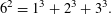
Euler [Reference Euler5, art. 249], in his 1770 Vollständige Anleitung zur Algebra, noted the relation
 $$\begin{eqnarray}6^{3}=3^{3}+4^{3}+5^{3}\end{eqnarray}$$
and asked for other instances of cubes that are sums of three consecutive cubes. Dickson’s History of the Theory of Numbers gives an extensive survey of early work on the problem of cubes that are sums of consecutive cubes [Reference Dickson4, pp. 582–585], and also squares that are sums of consecutive cubes [Reference Dickson4, pp. 585–588] with contributions by illustrious names such as Cunningham, Catalan, Gennochi and Lucas. Both problems possess some parametric families of solutions; one such family was constructed by Pagliani [Reference Pagliani11] in 1829:
 $$\begin{eqnarray}\biggl(\frac{v^{5}+v^{3}-2v}{6}\biggr)^{3}=\mathop{\sum }_{i=1}^{v^{3}}\biggl(\frac{v^{4}-3v^{3}-2v^{2}-2}{6}+i\biggr)^{3},\end{eqnarray}$$
where the congruence restriction
 $v\equiv 2$
or
$v\equiv 2$
or
 $4~(\text{mod}~6)$
ensures integrality of the cubes. Pagliani used this to answer a challenge, posed presumably by the editor Gergonne, of giving
$4~(\text{mod}~6)$
ensures integrality of the cubes. Pagliani used this to answer a challenge, posed presumably by the editor Gergonne, of giving
 $1000$
consecutive cubes whose sum is a cube. Of course, the problem of squares that are sums of consecutive cubes possesses the well-known parametric family of solutions
$1000$
consecutive cubes whose sum is a cube. Of course, the problem of squares that are sums of consecutive cubes possesses the well-known parametric family of solutions
 $$\begin{eqnarray}\biggl(\frac{d(d+1)}{2}\biggr)^{2}=\mathop{\sum }_{i=1}^{d}i^{3}=\mathop{\sum }_{i=0}^{d}i^{3}.\end{eqnarray}$$
These questions have continued to be of intermittent interest throughout a period of over 200 years. For example, Lucas [Reference Lucas8, p. 92] stated incorrectly that the only square expressible as a sum of three consecutive positive cubes is
 $$\begin{eqnarray}6^{2}=1^{3}+2^{3}+3^{3}.\end{eqnarray}$$
Both Cassels [Reference Cassels3] and Uchiyama [Reference Uchiyama17] determined the squares that can be written as sums of three consecutive cubes (without reference to Lucas), showing that the only solutions in addition to (2) are
 $$\begin{eqnarray}0=(-1)^{3}+0^{3}+1^{3},\qquad 3^{2}=0^{3}+1^{3}+2^{3},\qquad 204^{2}=23^{3}+24^{3}+25^{3}.\end{eqnarray}$$
Lucas also stated that the only square that is the sum of two consecutive positive cubes is
 $3^{2}=1^{3}+2^{3}$
and the only squares that are sums of five consecutive non-negative cubes are
$3^{2}=1^{3}+2^{3}$
and the only squares that are sums of five consecutive non-negative cubes are
 $$\begin{eqnarray}\displaystyle & \displaystyle 10^{2}=0^{3}+1^{3}+2^{3}+3^{3}+4^{3},\qquad 15^{2}=1^{3}+2^{3}+3^{3}+4^{3}+5^{3}, & \displaystyle \nonumber\\ \displaystyle & \displaystyle 315^{2}=25^{3}+26^{3}+27^{3}+28^{3}+29^{3}, & \displaystyle \nonumber\\ \displaystyle & \displaystyle 2170^{2}=96^{3}+97^{3}+98^{3}+99^{3}+100^{3}, & \displaystyle \nonumber\\ \displaystyle & \displaystyle 2940^{2}=118^{3}+119^{3}+120^{3}+121^{3}+122^{3}. & \displaystyle \nonumber\end{eqnarray}$$
These two claims turn out to be correct, as shown by Stroeker [Reference Stroeker16]. In modern language, the problem of which squares are expressible as the sum of
 $d$
consecutive cubes reduces, for any given
$d$
consecutive cubes reduces, for any given
 $d\geqslant 2$
, to the determination of integral points on a genus-
$d\geqslant 2$
, to the determination of integral points on a genus-
 $1$
curve. Stroeker [Reference Stroeker16], using a (by now) standard method based on linear forms in elliptic logarithms, solved this problem for
$1$
curve. Stroeker [Reference Stroeker16], using a (by now) standard method based on linear forms in elliptic logarithms, solved this problem for
 $2\leqslant d\leqslant 50$
.
$2\leqslant d\leqslant 50$
.
The problem of expressing arbitrary perfect powers as a sum of
 $d$
consecutive cubes with
$d$
consecutive cubes with
 $d$
small has received somewhat less attention, likely due to the fact that techniques for resolving such questions are of a much more recent vintage. Zhang [Reference Zhang19] showed that the only perfect powers that are sums of three consecutive cubes are precisely those already noted by Euler (1), Lucas (2) and Cassels (3). Zhang’s approach is to write the problem as
$d$
small has received somewhat less attention, likely due to the fact that techniques for resolving such questions are of a much more recent vintage. Zhang [Reference Zhang19] showed that the only perfect powers that are sums of three consecutive cubes are precisely those already noted by Euler (1), Lucas (2) and Cassels (3). Zhang’s approach is to write the problem as
 $$\begin{eqnarray}y^{n}=(x-1)^{3}+x^{3}+(x+1)^{3}=3x(x^{2}+2)\end{eqnarray}$$
and apply a descent argument that reduces this to certain ternary equations that have already been solved in the literature.
In this paper, we extend Stroeker’s aforementioned work, determining all perfect powers that are sums of
 $d$
consecutive cubes, with
$d$
consecutive cubes, with
 $2\leqslant d\leqslant 50$
. This upper bound is somewhat arbitrary as our techniques extend to essentially any fixed value of
$2\leqslant d\leqslant 50$
. This upper bound is somewhat arbitrary as our techniques extend to essentially any fixed value of
 $d$
.
$d$
.
Theorem 1. Let
 $2\leqslant d\leqslant 50$
. Let
$2\leqslant d\leqslant 50$
. Let
 $\ell$
be a prime. The integral solutions to the equation
$\ell$
be a prime. The integral solutions to the equation
 $$\begin{eqnarray}(x+1)^{3}+(x+2)^{3}+\cdots +(x+d)^{3}=y^{\ell }\end{eqnarray}$$
with
 $x\geqslant 1$
are given in Table 1.
$x\geqslant 1$
are given in Table 1.
Table 1 The solutions to equation (5) with
 $2\leqslant d\leqslant 50$
,
$2\leqslant d\leqslant 50$
,
 $\ell$
prime and
$\ell$
prime and
 $x\geqslant 1$
.
$x\geqslant 1$
.

The restriction
 $x\geqslant 1$
imposed in the statement of Theorem 1 is merely to exclude a multitude of artificial solutions. Solutions with
$x\geqslant 1$
imposed in the statement of Theorem 1 is merely to exclude a multitude of artificial solutions. Solutions with
 $x\leqslant 0$
can in fact be deduced easily, as we now explain.
$x\leqslant 0$
can in fact be deduced easily, as we now explain.
-
(i) The value
 $x=0$
gives the “trivial” solutions
$(x,y,\ell )=(0,d(d+1)/2,2)$
and no solutions for odd
$\ell$
. Likewise the value
$x=-1$
yields the trivial solutions
$(x,y,\ell )=(-1,(d-1)d/2,2)$
and no solutions for odd
$\ell$
.
$x=0$
gives the “trivial” solutions
$(x,y,\ell )=(0,d(d+1)/2,2)$
and no solutions for odd
$\ell$
. Likewise the value
$x=-1$
yields the trivial solutions
$(x,y,\ell )=(-1,(d-1)d/2,2)$
and no solutions for odd
$\ell$
. -
(ii) For odd exponents
$\ell$
, there is a symmetry between the solutions to (5): This allows us to deduce, from Table 1 and (i), all solutions with
$$\begin{eqnarray}(x,y,\ell )\longleftrightarrow (-x-d-1,-y,\ell ).\end{eqnarray}$$
$x\leqslant -d-1$
.
-
(iii) The solutions with
$-d\leqslant x\leqslant -2$
lead to non-negative solutions with smaller values of
$d$
through cancellation (and possibly applying the symmetry in (ii)).


Of course arbitrary perfect powers that are sums of at most
 $50$
consecutive cubes can be deduced from our list of
$50$
consecutive cubes can be deduced from our list of
 $\ell$
th powers with
$\ell$
th powers with
 $\ell$
prime.
$\ell$
prime.
A sum of
 $d$
consecutive cubes can be written as
$d$
consecutive cubes can be written as
 $$\begin{eqnarray}(x+1)^{3}+(x+2)^{3}+\cdots +(x+d)^{3}=\biggl(\!dx+\frac{d(d+1)}{2}\!\biggr)\biggl(x^{2}+(d+1)x+\frac{d(d+1)}{2}\biggr).\end{eqnarray}$$
Thus, to prove Theorem 1, we need to solve the Diophantine equation
 $$\begin{eqnarray}\biggl(dx+\frac{d(d+1)}{2}\biggr)\biggl(x^{2}+(d+1)x+\frac{d(d+1)}{2}\biggr)=y^{\ell }\end{eqnarray}$$
with
 $\ell$
prime and
$\ell$
prime and
 $2\leqslant d\leqslant 50$
. We find it convenient to rewrite (6) as
$2\leqslant d\leqslant 50$
. We find it convenient to rewrite (6) as
 $$\begin{eqnarray}d(2x+d+1)\biggl(x^{2}+(d+1)x+\frac{d(d+1)}{2}\biggr)=2y^{\ell }.\end{eqnarray}$$
We will use a descent argument together with the identity
 $$\begin{eqnarray}4\biggl(x^{2}+(d+1)x+\frac{d(d+1)}{2}\biggr)-(2x+d+1)^{2}=d^{2}-1,\end{eqnarray}$$
to reduce (7) to a family of ternary equations. The main purpose of this paper is to highlight the degree to which such ternary equations can, through a combination of techniques including descent, lower bounds for linear forms in logarithms and appeal to the modularity of Galois representations, be nowadays completely and explicitly solved.
2 Proof of Theorem 1 for
$\ell =2$

Although Theorem 1 with
 $\ell =2$
follows from Stroeker’s paper [Reference Stroeker16], we explain briefly how this can now be done with the help of an appropriate computer algebra package.
$\ell =2$
follows from Stroeker’s paper [Reference Stroeker16], we explain briefly how this can now be done with the help of an appropriate computer algebra package.
Let
 $(x,y)$
be an integral solution to (6) with
$(x,y)$
be an integral solution to (6) with
 $\ell =2$
. Write
$\ell =2$
. Write
 $X=dx$
and
$X=dx$
and
 $Y=dy$
. Then
$Y=dy$
. Then
 $(X,Y)$
is an integral point on the elliptic curve
$(X,Y)$
is an integral point on the elliptic curve
 $$\begin{eqnarray}E_{d}\;:\;Y^{2}=\biggl(X+\frac{d^{2}+d}{2}\biggr)\biggl(X^{2}+(d^{2}+d)X+\frac{d^{4}+d^{3}}{2}\biggr).\end{eqnarray}$$
Using the computer algebra package Magma [Reference Bosma, Cannon and Playoust1], we determined the integral points on
 $E_{d}$
for
$E_{d}$
for
 $2\leqslant d\leqslant 50$
. For this computation, Magma applies the standard linear forms in the elliptic logarithms method [Reference Smart15, Ch. XIII], which is the same method used by Stroeker (though the implementation is independent). From this we immediately recover the original solutions
$2\leqslant d\leqslant 50$
. For this computation, Magma applies the standard linear forms in the elliptic logarithms method [Reference Smart15, Ch. XIII], which is the same method used by Stroeker (though the implementation is independent). From this we immediately recover the original solutions
 $(x,y)$
to (6) with
$(x,y)$
to (6) with
 $\ell =2$
, and the latter are found in our Table 1. We have checked that our solutions with
$\ell =2$
, and the latter are found in our Table 1. We have checked that our solutions with
 $\ell =2$
are precisely those given by Stroeker.
$\ell =2$
are precisely those given by Stroeker.
We shall henceforth restrict ourselves to
 $\ell \geqslant 3$
.
$\ell \geqslant 3$
.
3 Proof of Theorem 1 for
$d=2$

Our method for general
 $d$
explained in later sections fails for
$d$
explained in later sections fails for
 $d=2$
. This is because of the presence of solutions
$d=2$
. This is because of the presence of solutions
 $(x,y)=(-2,-1)$
and
$(x,y)=(-2,-1)$
and
 $(x,y)=(-1,1)$
to (5) for all
$(x,y)=(-1,1)$
to (5) for all
 $\ell \geqslant 3$
. In this section, we treat the case
$\ell \geqslant 3$
. In this section, we treat the case
 $d=2$
separately, reducing to Diophantine equations that have already been solved by Nagell.
$d=2$
separately, reducing to Diophantine equations that have already been solved by Nagell.
We consider the equation (5) with
 $d=2$
. For convenience, let
$d=2$
. For convenience, let
 $z=x+1$
. The equation becomes
$z=x+1$
. The equation becomes
 $z^{3}+(z+1)^{3}=y^{\ell }$
, which can be rewritten as
$z^{3}+(z+1)^{3}=y^{\ell }$
, which can be rewritten as
 $$\begin{eqnarray}(2z+1)(z^{2}+z+1)=y^{\ell }.\end{eqnarray}$$
Here
 $y$
and
$y$
and
 $z$
are integers and
$z$
are integers and
 $\ell \geqslant 3$
is prime. Suppose first that
$\ell \geqslant 3$
is prime. Suppose first that
 $\ell =3$
. This equation here defines a genus-
$\ell =3$
. This equation here defines a genus-
 $1$
curve. We checked using Magma that it is isomorphic to the elliptic curve
$1$
curve. We checked using Magma that it is isomorphic to the elliptic curve
 $Y^{2}-9Y=X^{3}-27$
with Cremona label 27A1, and that it has Mordell–Weil group (over
$Y^{2}-9Y=X^{3}-27$
with Cremona label 27A1, and that it has Mordell–Weil group (over
 $\mathbb{Q}$
)
$\mathbb{Q}$
)
 $\cong \mathbb{Z}/3\mathbb{Z}$
. It follows that the only rational points on (9) with
$\cong \mathbb{Z}/3\mathbb{Z}$
. It follows that the only rational points on (9) with
 $\ell =3$
are the three obvious ones:
$\ell =3$
are the three obvious ones:
 $(z,y)=(-1/2,0)$
,
$(z,y)=(-1/2,0)$
,
 $(0,1)$
and
$(0,1)$
and
 $(-1,-1)$
. These yield the solutions
$(-1,-1)$
. These yield the solutions
 $(x,y)=(-1,1)$
and
$(x,y)=(-1,1)$
and
 $(x,y)=(-2,-1)$
to (5).
$(x,y)=(-2,-1)$
to (5).
We may thus suppose that
 $\ell \geqslant 5$
is prime. The resultant of the two factors on the left-hand side of (9) is
$\ell \geqslant 5$
is prime. The resultant of the two factors on the left-hand side of (9) is
 $3$
and, moreover,
$3$
and, moreover,
 $9\nmid (z^{2}+z+1)$
. It follows that either
$9\nmid (z^{2}+z+1)$
. It follows that either
 $$\begin{eqnarray}2z+1=y_{1}^{\ell },\qquad z^{2}+z+1=y_{2}^{\ell },\qquad y=y_{1}y_{2}\end{eqnarray}$$
or
 $$\begin{eqnarray}2z+1=3^{\ell -1}y_{1}^{n},\qquad z^{2}+z+1=3y_{2}^{\ell },\qquad y=3y_{1}y_{2}.\end{eqnarray}$$
Nagell [Reference Nagell10] showed that the only integer solutions to the equation
 $X^{2}+X+1=Y^{n}$
with
$X^{2}+X+1=Y^{n}$
with
 $n\neq 3^{k}$
are the trivial ones with
$n\neq 3^{k}$
are the trivial ones with
 $X=-1$
or
$X=-1$
or
 $0$
. Nagell [Reference Nagell10] also solved the equation
$0$
. Nagell [Reference Nagell10] also solved the equation
 $X^{2}+X+1=3Y^{n}$
for
$X^{2}+X+1=3Y^{n}$
for
 $n>2$
, showing that the only solutions are again the trivial ones with
$n>2$
, showing that the only solutions are again the trivial ones with
 $X=1$
. Working back, we see that the only solutions to (9) with
$X=1$
. Working back, we see that the only solutions to (9) with
 $\ell \geqslant 5$
are
$\ell \geqslant 5$
are
 $(z,y)=(0,1)$
and
$(z,y)=(0,1)$
and
 $(-1,-1)$
. These again give the solutions
$(-1,-1)$
. These again give the solutions
 $(x,y)=(-1,1)$
and
$(x,y)=(-1,1)$
and
 $(-2,-1)$
to (5).
$(-2,-1)$
to (5).
4 Descent for
$\ell \geqslant 5$

Let
 $d\geqslant 3$
. We consider equation (7) with exponent
$d\geqslant 3$
. We consider equation (7) with exponent
 $\ell \geqslant 5$
. The argument in this section will need modification for
$\ell \geqslant 5$
. The argument in this section will need modification for
 $\ell =3$
, which we carry out in §8. For a prime
$\ell =3$
, which we carry out in §8. For a prime
 $q$
, we let
$q$
, we let
 $$\begin{eqnarray}\unicode[STIX]{x1D707}_{q}=\text{ord}_{q}(d^{2}-1)\quad \text{and}\quad \unicode[STIX]{x1D708}_{q}=\text{ord}_{q}(d),\end{eqnarray}$$
i.e. the largest power of
 $q$
dividing
$q$
dividing
 $d^{2}-1$
and
$d^{2}-1$
and
 $d$
, respectively. We associate to
$d$
, respectively. We associate to
 $q$
a finite subset
$q$
a finite subset
 $T_{q}\subset \mathbb{Z}^{2}$
as follows.
$T_{q}\subset \mathbb{Z}^{2}$
as follows.
-
∙ If
$q\nmid d(d^{2}-1)$
, then let
$T_{q}=\{(0,0)\}$
. -
∙ For
$q=2$
, we define
$$\begin{eqnarray}T_{2}=\left\{\begin{array}{@{}ll@{}}\{(0,1-\unicode[STIX]{x1D708}_{2})\}\quad & \text{if }2\mid d,\\ \{(1,0),(\unicode[STIX]{x1D707}_{2}/2,1-\unicode[STIX]{x1D707}_{2}/2),(3-\unicode[STIX]{x1D707}_{2},\unicode[STIX]{x1D707}_{2}-2)\}\quad & \text{if }2\nmid d\text{ and }2\mid \unicode[STIX]{x1D707}_{2},\\ \{(1,0),(3-\unicode[STIX]{x1D707}_{2},\unicode[STIX]{x1D707}_{2}-2)\}\quad & \text{if }2\nmid d\text{ and }2\nmid \unicode[STIX]{x1D707}_{2}.\end{array}\right.\end{eqnarray}$$
-
∙ For odd
$q\mid d$
, let
$$\begin{eqnarray}T_{q}=\{(-\unicode[STIX]{x1D708}_{q},0),(0,-\unicode[STIX]{x1D708}_{q})\}.\end{eqnarray}$$
-
∙ For odd
$q\mid (d^{2}-1)$
, let
$$\begin{eqnarray}T_{q}=\left\{\begin{array}{@{}ll@{}}\{(0,0),(-\unicode[STIX]{x1D707}_{q},\unicode[STIX]{x1D707}_{q}),(\unicode[STIX]{x1D707}_{q}/2,-\unicode[STIX]{x1D707}_{q}/2)\}\quad & \text{if }2\mid \unicode[STIX]{x1D707}_{q},\\ \{(0,0),(-\unicode[STIX]{x1D707}_{q},\unicode[STIX]{x1D707}_{q})\}\quad & \text{if }2\nmid \unicode[STIX]{x1D707}_{q}.\end{array}\right.\end{eqnarray}$$


We take
 ${\mathcal{A}}_{d}$
to be the set of pairs of positive rationals
${\mathcal{A}}_{d}$
to be the set of pairs of positive rationals
 $(\unicode[STIX]{x1D6FC},\unicode[STIX]{x1D6FD})$
such that
$(\unicode[STIX]{x1D6FC},\unicode[STIX]{x1D6FD})$
such that
 $$\begin{eqnarray}(\text{ord}_{q}(\unicode[STIX]{x1D6FC}),\text{ord}_{q}(\unicode[STIX]{x1D6FD}))\in T_{q}\end{eqnarray}$$
for all primes
 $q$
. It is clear that
$q$
. It is clear that
 ${\mathcal{A}}_{d}$
is a finite set, which is, in practice, easy to write down for any value of
${\mathcal{A}}_{d}$
is a finite set, which is, in practice, easy to write down for any value of
 $d$
.
$d$
.
Lemma 4.1. Let
 $(x,y)$
be a solution to (7), where
$(x,y)$
be a solution to (7), where
 $\ell \geqslant 5$
is a prime. Then there are rationals
$\ell \geqslant 5$
is a prime. Then there are rationals
 $y_{1}$
,
$y_{1}$
,
 $y_{2}$
and a pair
$y_{2}$
and a pair
 $(\unicode[STIX]{x1D6FC},\unicode[STIX]{x1D6FD})\in {\mathcal{A}}_{d}$
such that
$(\unicode[STIX]{x1D6FC},\unicode[STIX]{x1D6FD})\in {\mathcal{A}}_{d}$
such that
 $$\begin{eqnarray}2x+d+1=\unicode[STIX]{x1D6FC}y_{1}^{\ell },\qquad x^{2}+(d+1)x+\frac{d(d+1)}{2}=\unicode[STIX]{x1D6FD}y_{2}^{\ell }.\end{eqnarray}$$
Moreover, if
 $3\leqslant d\leqslant 50$
, then
$3\leqslant d\leqslant 50$
, then
 $y_{1}$
and
$y_{1}$
and
 $y_{2}$
are integers.
$y_{2}$
are integers.
Remark.
The reader will observe that the definition of
 ${\mathcal{A}}_{d}$
is independent of
${\mathcal{A}}_{d}$
is independent of
 $\ell$
. Thus, given
$\ell$
. Thus, given
 $d$
, the lemma provides us with a way of carrying out the descent uniformly for all
$d$
, the lemma provides us with a way of carrying out the descent uniformly for all
 $\ell \geqslant 5$
.
$\ell \geqslant 5$
.
Proof. Let us first assume the first part of the lemma and deduce the second. Using a short Magma script, we wrote down all possible pairs
 $(\unicode[STIX]{x1D6FC},\unicode[STIX]{x1D6FD})\in {\mathcal{A}}_{d}$
for
$(\unicode[STIX]{x1D6FC},\unicode[STIX]{x1D6FD})\in {\mathcal{A}}_{d}$
for
 $3\leqslant d\leqslant 50$
and checked that
$3\leqslant d\leqslant 50$
and checked that
 $$\begin{eqnarray}\max \{\text{ord}_{q}(\unicode[STIX]{x1D6FC}),\text{ord}_{q}(\unicode[STIX]{x1D6FD})\}\leqslant 4\end{eqnarray}$$
for all primes
 $q$
. As
$q$
. As
 $x$
is an integer, we know from (11) that
$x$
is an integer, we know from (11) that
 $$\begin{eqnarray}\text{ord}_{q}(\unicode[STIX]{x1D6FC})+\ell \,\text{ord}_{q}(y_{1})\geqslant 0\quad \text{and}\quad \text{ord}_{q}(\unicode[STIX]{x1D6FD})+\ell \,\text{ord}_{q}(y_{2})\geqslant 0\end{eqnarray}$$
for all primes
 $q$
. Since
$q$
. Since
 $\ell \geqslant 5$
, it is clear that
$\ell \geqslant 5$
, it is clear that
 $\text{ord}_{q}(y_{1})\geqslant 0$
and
$\text{ord}_{q}(y_{1})\geqslant 0$
and
 $\text{ord}_{q}(y_{2})\geqslant 0$
for all primes
$\text{ord}_{q}(y_{2})\geqslant 0$
for all primes
 $q$
. This proves the second part of the lemma.
$q$
. This proves the second part of the lemma.
We now prove the first part of the lemma. For
 $2x+d+1=0$
(which can only arise for odd values of
$2x+d+1=0$
(which can only arise for odd values of
 $d$
), we can take
$d$
), we can take
 $y_{1}=0$
,
$y_{1}=0$
,
 $y_{2}=1$
,
$y_{2}=1$
,
 $$\begin{eqnarray}\unicode[STIX]{x1D6FC}=\frac{8}{d(d^{2}-1)}\quad \text{and}\quad \unicode[STIX]{x1D6FD}=\frac{d^{2}-1}{4};\end{eqnarray}$$
it is easy to check that this particular pair
 $(\unicode[STIX]{x1D6FC},\unicode[STIX]{x1D6FD})$
belongs to
$(\unicode[STIX]{x1D6FC},\unicode[STIX]{x1D6FD})$
belongs to
 ${\mathcal{A}}_{d}$
. We shall henceforth suppose that
${\mathcal{A}}_{d}$
. We shall henceforth suppose that
 $2x+d+1\neq 0$
.
$2x+d+1\neq 0$
.
Claim.
Let
 $q$
be a prime and define
$q$
be a prime and define
 $$\begin{eqnarray}\unicode[STIX]{x1D716}=\text{ord}_{q}(2x+d+1)\quad \text{and}\quad \unicode[STIX]{x1D6FF}=\text{ord}_{q}\biggl(x^{2}+(d+1)x+\frac{d(d+1)}{2}\biggr).\end{eqnarray}$$
Then
 $(\unicode[STIX]{x1D716},\unicode[STIX]{x1D6FF})\equiv (\unicode[STIX]{x1D716}^{\prime },\unicode[STIX]{x1D6FF}^{\prime })~(\text{mod}~\ell )$
for some
$(\unicode[STIX]{x1D716},\unicode[STIX]{x1D6FF})\equiv (\unicode[STIX]{x1D716}^{\prime },\unicode[STIX]{x1D6FF}^{\prime })~(\text{mod}~\ell )$
for some
 $(\unicode[STIX]{x1D716}^{\prime },\unicode[STIX]{x1D6FF}^{\prime })\in T_{q}$
.
$(\unicode[STIX]{x1D716}^{\prime },\unicode[STIX]{x1D6FF}^{\prime })\in T_{q}$
.
To complete the proof of Lemma 4.1, it is clearly enough to prove this claim. From (7) and (8), the claim is certainly true if
 $q\nmid d(d^{2}-1)$
, so we may suppose that
$q\nmid d(d^{2}-1)$
, so we may suppose that
 $q\mid d(d^{2}-1)$
. Observe that for any
$q\mid d(d^{2}-1)$
. Observe that for any
 $q$
, from (7),
$q$
, from (7),
 $$\begin{eqnarray}\unicode[STIX]{x1D708}_{q}+\unicode[STIX]{x1D716}+\unicode[STIX]{x1D6FF}\equiv \text{ord}_{q}(2)\quad (\text{mod}~\ell ).\end{eqnarray}$$
Moreover, from (8),
 $$\begin{eqnarray}\unicode[STIX]{x1D707}_{q}\geqslant \min (2\unicode[STIX]{x1D716},\unicode[STIX]{x1D6FF}+2\,\text{ord}_{q}(2))\quad \text{with equality if}\;2\unicode[STIX]{x1D716}\neq \unicode[STIX]{x1D6FF}+2\,\text{ord}_{q}(2).\end{eqnarray}$$
We deal first with the case where
 $q=2\mid d$
(so that
$q=2\mid d$
(so that
 $\unicode[STIX]{x1D716}=0$
). By (13), we obtain that
$\unicode[STIX]{x1D716}=0$
). By (13), we obtain that
 $(\unicode[STIX]{x1D716},\unicode[STIX]{x1D6FF})\equiv (0,1-\unicode[STIX]{x1D708}_{2})~(\text{mod}~\ell )$
and, by definition,
$(\unicode[STIX]{x1D716},\unicode[STIX]{x1D6FF})\equiv (0,1-\unicode[STIX]{x1D708}_{2})~(\text{mod}~\ell )$
and, by definition,
 $T_{2}=\{(0,1-\unicode[STIX]{x1D708}_{2})\}$
, establishing our claim. Next we suppose that
$T_{2}=\{(0,1-\unicode[STIX]{x1D708}_{2})\}$
, establishing our claim. Next we suppose that
 $q=2\nmid d$
(in which case
$q=2\nmid d$
(in which case
 $\unicode[STIX]{x1D708}_{2}=0$
).
$\unicode[STIX]{x1D708}_{2}=0$
).
-
∙ If
$2\unicode[STIX]{x1D716}=\unicode[STIX]{x1D6FF}+2$
, then, from (13) and the fact that
$\ell \geqslant 5$
, we obtain
$(\unicode[STIX]{x1D716},\unicode[STIX]{x1D6FF})\equiv (1,0)~(\text{mod}~\ell )$
. -
∙ If
$2\unicode[STIX]{x1D716}>\unicode[STIX]{x1D6FF}+2$
, then, from (14), we have
$\unicode[STIX]{x1D707}_{2}=\unicode[STIX]{x1D6FF}+2$
, so from (13) we obtain
$(\unicode[STIX]{x1D716},\unicode[STIX]{x1D6FF})\equiv (3-\unicode[STIX]{x1D707}_{2},\unicode[STIX]{x1D707}_{2}-2)~(\text{mod}~\ell )$
. -
∙ If
$2\unicode[STIX]{x1D716}<\unicode[STIX]{x1D6FF}+2$
, then, from (14), we have
$\unicode[STIX]{x1D707}_{2}=2\unicode[STIX]{x1D716}$
, so from (13) we obtain
$(\unicode[STIX]{x1D716},\unicode[STIX]{x1D6FF})\equiv (\unicode[STIX]{x1D707}_{2}/2,1-\unicode[STIX]{x1D707}_{2}/2)~(\text{mod}~\ell )$
.


Next, let us next consider odd
 $q\mid d$
(whereby we have that
$q\mid d$
(whereby we have that
 $\unicode[STIX]{x1D707}_{q}=0$
). From (14), it follows that either
$\unicode[STIX]{x1D707}_{q}=0$
). From (14), it follows that either
 $\unicode[STIX]{x1D716}=0$
or
$\unicode[STIX]{x1D716}=0$
or
 $\unicode[STIX]{x1D6FF}=0$
. From (13), we obtain
$\unicode[STIX]{x1D6FF}=0$
. From (13), we obtain
 $(\unicode[STIX]{x1D716},\unicode[STIX]{x1D6FF})\equiv (0,-\unicode[STIX]{x1D708}_{q})$
or
$(\unicode[STIX]{x1D716},\unicode[STIX]{x1D6FF})\equiv (0,-\unicode[STIX]{x1D708}_{q})$
or
 $(-\unicode[STIX]{x1D708}_{q},0)~(\text{mod}~\ell )$
, as required.
$(-\unicode[STIX]{x1D708}_{q},0)~(\text{mod}~\ell )$
, as required.
Finally we consider odd
 $q\mid (d^{2}-1)$
(so
$q\mid (d^{2}-1)$
(so
 $\unicode[STIX]{x1D708}_{q}=0$
).
$\unicode[STIX]{x1D708}_{q}=0$
).
-
∙ If
$2\unicode[STIX]{x1D716}=\unicode[STIX]{x1D6FF}$
, then, from (13) and the fact that
$\ell \geqslant 5$
, we obtain
$(\unicode[STIX]{x1D716},\unicode[STIX]{x1D6FF})\equiv (0,0)~(\text{mod}~\ell )$
. -
∙ If
$2\unicode[STIX]{x1D716}>\unicode[STIX]{x1D6FF}$
, then, from (14), we have
$\unicode[STIX]{x1D707}_{q}=\unicode[STIX]{x1D6FF}$
, so from (13) we obtain
$(\unicode[STIX]{x1D716},\unicode[STIX]{x1D6FF})\equiv (-\unicode[STIX]{x1D707}_{q},\unicode[STIX]{x1D707}_{q})~(\text{mod}~\ell )$
. -
∙ If
$2\unicode[STIX]{x1D716}<\unicode[STIX]{x1D6FF}$
, then, from (14), we have
$\unicode[STIX]{x1D707}_{q}=2\unicode[STIX]{x1D716}$
, so from (13) we obtain
$(\unicode[STIX]{x1D716},\unicode[STIX]{x1D6FF})\equiv (\unicode[STIX]{x1D707}_{q}/2,-\unicode[STIX]{x1D707}_{q}/2)~(\text{mod}~\ell )$
. ◻


From (11) and (8), we deduce the following ternary equation:
 $$\begin{eqnarray}4\unicode[STIX]{x1D6FD}y_{2}^{\ell }-\unicode[STIX]{x1D6FC}^{2}y_{1}^{2\ell }=d^{2}-1.\end{eqnarray}$$
We need to solve this for each possible
 $(\unicode[STIX]{x1D6FC},\unicode[STIX]{x1D6FD})\in {\mathcal{A}}_{d}$
with
$(\unicode[STIX]{x1D6FC},\unicode[STIX]{x1D6FD})\in {\mathcal{A}}_{d}$
with
 $2\leqslant d\leqslant 50$
and
$2\leqslant d\leqslant 50$
and
 $y_{1}$
,
$y_{1}$
,
 $y_{2}$
integers. Clearing denominators and dividing by the greatest common divisor of the coefficients, we can rewrite this as
$y_{2}$
integers. Clearing denominators and dividing by the greatest common divisor of the coefficients, we can rewrite this as
 $$\begin{eqnarray}ry_{2}^{\ell }-sy_{1}^{2\ell }=t,\end{eqnarray}$$
where
 $r$
,
$r$
,
 $s$
,
$s$
,
 $t$
are positive integers and
$t$
are positive integers and
 $\text{gcd}(r,s,t)=1$
.
$\text{gcd}(r,s,t)=1$
.
5 Linear forms in two logarithms
The descent step in the previous section transforms (7) into a family of ternary equations (15). In this section, we appeal to lower bounds for linear forms in logarithms to bound the exponent
 $\ell$
appearing in these equations. We will use a special case of Corollary 2 of Laurent [Reference Laurent7] (with
$\ell$
appearing in these equations. We will use a special case of Corollary 2 of Laurent [Reference Laurent7] (with
 $m=10$
in the notation of that paper).
$m=10$
in the notation of that paper).
Proposition 5.1. Let
 $\unicode[STIX]{x1D6FC}_{1}$
and
$\unicode[STIX]{x1D6FC}_{1}$
and
 $\unicode[STIX]{x1D6FC}_{2}$
be positive real, multiplicatively independent algebraic numbers and
$\unicode[STIX]{x1D6FC}_{2}$
be positive real, multiplicatively independent algebraic numbers and
 $\log \unicode[STIX]{x1D6FC}_{1}$
and
$\log \unicode[STIX]{x1D6FC}_{1}$
and
 $\log \unicode[STIX]{x1D6FC}_{2}$
be any fixed determinations of their logarithms that are real and positive. Write
$\log \unicode[STIX]{x1D6FC}_{2}$
be any fixed determinations of their logarithms that are real and positive. Write
 $D=[\mathbb{Q}(\unicode[STIX]{x1D6FC}_{1},\unicode[STIX]{x1D6FC}_{2}):\mathbb{Q}]$
and
$D=[\mathbb{Q}(\unicode[STIX]{x1D6FC}_{1},\unicode[STIX]{x1D6FC}_{2}):\mathbb{Q}]$
and
 $$\begin{eqnarray}b^{\prime }=\frac{b_{1}}{D\log A_{2}}+\frac{b_{2}}{D\log A_{1}},\end{eqnarray}$$
where
 $b_{1}$
and
$b_{1}$
and
 $b_{2}$
are positive integers and
$b_{2}$
are positive integers and
 $A_{1}$
and
$A_{1}$
and
 $A_{2}$
are real numbers
$A_{2}$
are real numbers
 ${>}1$
such that
${>}1$
such that
 $$\begin{eqnarray}\log A_{i}\geqslant \max \{h(\unicode[STIX]{x1D6FC}_{i}),|\text{log}\,\unicode[STIX]{x1D6FC}_{i}|/D,1/D\},\quad i=1,2.\end{eqnarray}$$
Let
 $\unicode[STIX]{x1D6EC}=b_{2}\log \unicode[STIX]{x1D6FC}_{2}-b_{1}\log \unicode[STIX]{x1D6FC}_{1}$
. Then
$\unicode[STIX]{x1D6EC}=b_{2}\log \unicode[STIX]{x1D6FC}_{2}-b_{1}\log \unicode[STIX]{x1D6FC}_{1}$
. Then
 $$\begin{eqnarray}\log |\unicode[STIX]{x1D6EC}|\geqslant -25.2D^{4}(\max \{\log b^{\prime }+0.38,10/D,1\})^{2}\log A_{1}\log A_{2}.\end{eqnarray}$$
Here, we have defined, as usual, the absolute logarithmic height of an algebraic number
 $\unicode[STIX]{x1D6FC}$
by
$\unicode[STIX]{x1D6FC}$
by
 $$\begin{eqnarray}h(\unicode[STIX]{x1D6FC})=\frac{1}{d}\biggl(\log |a|+\mathop{\sum }_{i=1}^{d}\log \max (1,|\unicode[STIX]{x1D6FC}^{(i)}|)\biggr),\end{eqnarray}$$
where
 $a$
is the leading coefficient of the minimal polynomial of
$a$
is the leading coefficient of the minimal polynomial of
 $\unicode[STIX]{x1D6FC}$
and the
$\unicode[STIX]{x1D6FC}$
and the
 $\unicode[STIX]{x1D6FC}^{(i)}$
are the conjugates of
$\unicode[STIX]{x1D6FC}^{(i)}$
are the conjugates of
 $\unicode[STIX]{x1D6FC}$
in
$\unicode[STIX]{x1D6FC}$
in
 $\mathbb{C}$
.
$\mathbb{C}$
.
In this section, we will assume that
 $3\leqslant d\leqslant 50$
. In the notation of the previous section,
$3\leqslant d\leqslant 50$
. In the notation of the previous section,
 $(\unicode[STIX]{x1D6FC},\unicode[STIX]{x1D6FD})$
will denote an element of
$(\unicode[STIX]{x1D6FC},\unicode[STIX]{x1D6FD})$
will denote an element of
 ${\mathcal{A}}_{d}$
while
${\mathcal{A}}_{d}$
while
 $(y_{1},y_{2})$
denotes an integral solution to (15). By definition of
$(y_{1},y_{2})$
denotes an integral solution to (15). By definition of
 ${\mathcal{A}}_{d}$
, the rationals
${\mathcal{A}}_{d}$
, the rationals
 $\unicode[STIX]{x1D6FC}$
and
$\unicode[STIX]{x1D6FC}$
and
 $\unicode[STIX]{x1D6FD}$
are both positive. It follows from (15) that
$\unicode[STIX]{x1D6FD}$
are both positive. It follows from (15) that
 $y_{2}>0$
.
$y_{2}>0$
.
Lemma 5.2. Let
 $\ell >1000$
. Suppose that
$\ell >1000$
. Suppose that
 $|y_{1}|$
,
$|y_{1}|$
,
 $y_{2}\geqslant 2$
and
$y_{2}\geqslant 2$
and
 $y_{2}\neq y_{1}^{2}$
. Let
$y_{2}\neq y_{1}^{2}$
. Let
 $$\begin{eqnarray}\unicode[STIX]{x1D6FC}_{1}=4\unicode[STIX]{x1D6FD}/\unicode[STIX]{x1D6FC}^{2}\quad \text{and}\quad \unicode[STIX]{x1D6FC}_{2}=y_{1}^{2}/y_{2}.\end{eqnarray}$$
Then
 $\unicode[STIX]{x1D6FC}_{1}$
and
$\unicode[STIX]{x1D6FC}_{1}$
and
 $\unicode[STIX]{x1D6FC}_{2}$
are positive and multiplicatively independent. Moreover, writing
$\unicode[STIX]{x1D6FC}_{2}$
are positive and multiplicatively independent. Moreover, writing
 $$\begin{eqnarray}\unicode[STIX]{x1D6EC}=\log \unicode[STIX]{x1D6FC}_{1}-\ell \log \unicode[STIX]{x1D6FC}_{2},\end{eqnarray}$$
we have
 $$\begin{eqnarray}0<\unicode[STIX]{x1D6EC}<\frac{d^{2}-1}{\unicode[STIX]{x1D6FC}^{2}y_{1}^{2\ell }}.\end{eqnarray}$$
Proof. By the observation preceding the statement of the lemma, we know that
 $\unicode[STIX]{x1D6FC}_{1}$
and
$\unicode[STIX]{x1D6FC}_{1}$
and
 $\unicode[STIX]{x1D6FC}_{2}$
are positive. From (15), (17), (18) and (19), we have
$\unicode[STIX]{x1D6FC}_{2}$
are positive. From (15), (17), (18) and (19), we have
 $$\begin{eqnarray}\text{e}^{\unicode[STIX]{x1D6EC}}-1=\frac{4\unicode[STIX]{x1D6FD}}{\unicode[STIX]{x1D6FC}^{2}}\cdot \frac{y_{2}^{\ell }}{y_{1}^{2\ell }}-1=\frac{d^{2}-1}{\unicode[STIX]{x1D6FC}^{2}y_{1}^{2\ell }}>0,\end{eqnarray}$$
whence
 $\unicode[STIX]{x1D6EC}>0$
. The second part of the lemma thus follows from the inequality
$\unicode[STIX]{x1D6EC}>0$
. The second part of the lemma thus follows from the inequality
 $\text{e}^{\unicode[STIX]{x1D6EC}}-1>\unicode[STIX]{x1D6EC}$
.
$\text{e}^{\unicode[STIX]{x1D6EC}}-1>\unicode[STIX]{x1D6EC}$
.
It remains to show the multiplicative independence of
 $\unicode[STIX]{x1D6FC}_{1}$
and
$\unicode[STIX]{x1D6FC}_{1}$
and
 $\unicode[STIX]{x1D6FC}_{2}$
, so suppose, for a contradiction, that they are multiplicatively dependent. Thus, there exist coprime positive integers
$\unicode[STIX]{x1D6FC}_{2}$
, so suppose, for a contradiction, that they are multiplicatively dependent. Thus, there exist coprime positive integers
 $u$
and
$u$
and
 $v$
such that
$v$
such that
 $\unicode[STIX]{x1D6FC}_{1}^{u}=\unicode[STIX]{x1D6FC}_{2}^{v}$
. If
$\unicode[STIX]{x1D6FC}_{1}^{u}=\unicode[STIX]{x1D6FC}_{2}^{v}$
. If
 $\unicode[STIX]{x1D6FC}_{1}=1$
, then
$\unicode[STIX]{x1D6FC}_{1}=1$
, then
 $\unicode[STIX]{x1D6FC}_{2}=1$
, so that
$\unicode[STIX]{x1D6FC}_{2}=1$
, so that
 $y_{2}=y_{1}^{2}$
, contradicting the hypotheses of the lemma. Thus,
$y_{2}=y_{1}^{2}$
, contradicting the hypotheses of the lemma. Thus,
 $\unicode[STIX]{x1D6FC}_{1}\neq 1$
. Defining
$\unicode[STIX]{x1D6FC}_{1}\neq 1$
. Defining
 $$\begin{eqnarray}g=\text{gcd}\{\text{ord}_{p}(\unicode[STIX]{x1D6FC}_{1}):p\text{ prime}\},\end{eqnarray}$$
as
 $\unicode[STIX]{x1D6FC}_{1}\neq 1$
, we necessarily have
$\unicode[STIX]{x1D6FC}_{1}\neq 1$
, we necessarily have
 $g\neq 0$
. Clearly
$g\neq 0$
. Clearly
 $v\mid g$
. However, from (18),
$v\mid g$
. However, from (18),
 $$\begin{eqnarray}\unicode[STIX]{x1D6EC}=(\log \unicode[STIX]{x1D6FC}_{1})\biggl(1-\ell \frac{\log \unicode[STIX]{x1D6FC}_{2}}{\log \unicode[STIX]{x1D6FC}_{1}}\biggr)=(\log \unicode[STIX]{x1D6FC}_{1})\biggl(1-\ell \frac{u}{v}\biggr)=|\text{log}\,\unicode[STIX]{x1D6FC}_{1}|\cdot \biggl|1-\ell \frac{u}{v}\biggr|.\end{eqnarray}$$
From (19), we have
 $$\begin{eqnarray}0<\biggl|1-\ell \frac{u}{v}\biggr|<\frac{d^{2}-1}{|\text{log}\,\unicode[STIX]{x1D6FC}_{1}|\cdot \unicode[STIX]{x1D6FC}^{2}y_{1}^{2\ell }}.\end{eqnarray}$$
Now the non-zero rational
 $1-\ell u/v$
has denominator dividing
$1-\ell u/v$
has denominator dividing
 $v$
and hence dividing
$v$
and hence dividing
 $g$
. Thus,
$g$
. Thus,
 $$\begin{eqnarray}\frac{1}{g}\leqslant \biggl|1-\ell \frac{u}{v}\biggr|.\end{eqnarray}$$
Since
 $|y_{1}|\geqslant 2$
, it follows that
$|y_{1}|\geqslant 2$
, it follows that
 $$\begin{eqnarray}4^{\ell }\leqslant y_{1}^{2\ell }<\frac{(d^{2}-1)g}{|\text{log}\,\unicode[STIX]{x1D6FC}_{1}|\cdot \unicode[STIX]{x1D6FC}^{2}},\end{eqnarray}$$
and so
 $$\begin{eqnarray}\ell <\log \biggl(\frac{(d^{2}-1)g}{|\text{log}\unicode[STIX]{x1D6FC}_{1}|\cdot \unicode[STIX]{x1D6FC}^{2}}\biggr)/\log 4.\end{eqnarray}$$
We wrote a simple Magma script that computes this bound on
 $\ell$
for the values of
$\ell$
for the values of
 $d$
in the range
$d$
in the range
 $3\leqslant d\leqslant 50$
and the possible pairs
$3\leqslant d\leqslant 50$
and the possible pairs
 $(\unicode[STIX]{x1D6FC},\unicode[STIX]{x1D6FD})\in {\mathcal{A}}_{d}$
with corresponding
$(\unicode[STIX]{x1D6FC},\unicode[STIX]{x1D6FD})\in {\mathcal{A}}_{d}$
with corresponding
 $\unicode[STIX]{x1D6FC}_{1}=4\unicode[STIX]{x1D6FD}/\unicode[STIX]{x1D6FC}^{2}\neq 1$
. We found that the largest possible value for the right-hand side of the inequality is
$\unicode[STIX]{x1D6FC}_{1}=4\unicode[STIX]{x1D6FD}/\unicode[STIX]{x1D6FC}^{2}\neq 1$
. We found that the largest possible value for the right-hand side of the inequality is
 $19.09\ldots$
corresponding to
$19.09\ldots$
corresponding to
 $d=50$
and
$d=50$
and
 $(\unicode[STIX]{x1D6FC},\unicode[STIX]{x1D6FD})=(1/62\,475,2499)$
. As
$(\unicode[STIX]{x1D6FC},\unicode[STIX]{x1D6FD})=(1/62\,475,2499)$
. As
 $\ell >1000$
, we have a contradiction by a wide margin.
$\ell >1000$
, we have a contradiction by a wide margin.
In fact, we found only one pair
 $(\unicode[STIX]{x1D6FC},\unicode[STIX]{x1D6FD})$
for which
$(\unicode[STIX]{x1D6FC},\unicode[STIX]{x1D6FD})$
for which
 $\unicode[STIX]{x1D6FC}_{1}=1$
. This arises when
$\unicode[STIX]{x1D6FC}_{1}=1$
. This arises when
 $d=8$
and
$d=8$
and
 $(\unicode[STIX]{x1D6FC},\unicode[STIX]{x1D6FD})=(1,1/4)$
.◻
$(\unicode[STIX]{x1D6FC},\unicode[STIX]{x1D6FD})=(1,1/4)$
.◻
Lemma 5.3. Let
 $A_{2}=\max \{y_{1}^{2},y_{2}\}$
. Under the notation and assumptions of the previous lemma,
$A_{2}=\max \{y_{1}^{2},y_{2}\}$
. Under the notation and assumptions of the previous lemma,
 $$\begin{eqnarray}1\leqslant \frac{\log A_{2}}{\log y_{1}^{2}}\leqslant 1.03.\end{eqnarray}$$
Proof. It is sufficient to show that
 $\log y_{2}/\text{log}\,y_{1}^{2}\leqslant 1.03$
. From (17), (18) and (19), we have
$\log y_{2}/\text{log}\,y_{1}^{2}\leqslant 1.03$
. From (17), (18) and (19), we have
 $$\begin{eqnarray}\text{log}\,\unicode[STIX]{x1D6FC}_{1}-\ell (\log y_{1}^{2}-\log y_{2})<\frac{d^{2}-1}{\unicode[STIX]{x1D6FC}^{2}\cdot 4^{\ell }},\end{eqnarray}$$
where we have used the assumption
 $|y_{1}|\geqslant 2$
. It follows that
$|y_{1}|\geqslant 2$
. It follows that
 $$\begin{eqnarray}\displaystyle \frac{\log y_{2}}{\log y_{1}^{2}} & {<} & \displaystyle 1+\frac{1}{\ell \log y_{1}^{2}}\biggl(-\log \unicode[STIX]{x1D6FC}_{1}+\frac{(d^{2}-1)}{\unicode[STIX]{x1D6FC}^{2}\cdot 4^{\ell }}\biggr)\nonumber\\ \displaystyle & {\leqslant} & \displaystyle 1+\frac{1}{\ell \log y_{1}^{2}}\biggl(|\text{log}\,\unicode[STIX]{x1D6FC}_{1}|+\frac{(d^{2}-1)}{\unicode[STIX]{x1D6FC}^{2}\cdot 4^{\ell }}\biggr)\nonumber\\ \displaystyle & {<} & \displaystyle 1+\frac{1}{1000\log 4}\biggl(|\text{log}\,\unicode[STIX]{x1D6FC}_{1}|+\frac{(d^{2}-1)}{\unicode[STIX]{x1D6FC}^{2}\cdot 4^{1000}}\biggr),\nonumber\end{eqnarray}$$
using the assumptions
 $\ell >1000$
and
$\ell >1000$
and
 $|y_{1}|\geqslant 2$
. We wrote a Magma script that computed this upper bound for
$|y_{1}|\geqslant 2$
. We wrote a Magma script that computed this upper bound for
 $\log y_{1}^{2}/\text{log}\,y_{2}$
for all
$\log y_{1}^{2}/\text{log}\,y_{2}$
for all
 $3\leqslant d\leqslant 50$
and
$3\leqslant d\leqslant 50$
and
 $(\unicode[STIX]{x1D6FC},\unicode[STIX]{x1D6FD})\in {\mathcal{A}}_{d}$
. The largest value of the upper bound we obtained was
$(\unicode[STIX]{x1D6FC},\unicode[STIX]{x1D6FD})\in {\mathcal{A}}_{d}$
. The largest value of the upper bound we obtained was
 $1.02257\ldots ,$
again corresponding to
$1.02257\ldots ,$
again corresponding to
 $d=50$
and
$d=50$
and
 $(\unicode[STIX]{x1D6FC},\unicode[STIX]{x1D6FD})=(1/62\,475,2499)$
. This completes the proof.◻
$(\unicode[STIX]{x1D6FC},\unicode[STIX]{x1D6FD})=(1/62\,475,2499)$
. This completes the proof.◻
We continue under the assumptions of Lemma 5.2, applying Proposition 5.1 to obtain a bound for the exponent
 $\ell$
. We let
$\ell$
. We let
 $$\begin{eqnarray}A_{1}=\max \{H(\unicode[STIX]{x1D6FC}_{1}),e\},\end{eqnarray}$$
where
 $H(u/v)$
, for coprime integers
$H(u/v)$
, for coprime integers
 $u$
,
$u$
,
 $v$
(with
$v$
(with
 $v$
non-zero), is simply
$v$
non-zero), is simply
 $\max \{|u|,|v|\}$
. Let
$\max \{|u|,|v|\}$
. Let
 $A_{2}$
be as in Lemma 5.3. We see, thanks to Lemma 5.2, that the hypotheses of Proposition 5.1 are satisfied for our choices of
$A_{2}$
be as in Lemma 5.3. We see, thanks to Lemma 5.2, that the hypotheses of Proposition 5.1 are satisfied for our choices of
 $\unicode[STIX]{x1D6FC}_{1}$
,
$\unicode[STIX]{x1D6FC}_{1}$
,
 $\unicode[STIX]{x1D6FC}_{2}$
,
$\unicode[STIX]{x1D6FC}_{2}$
,
 $A_{1}$
and
$A_{1}$
and
 $A_{2}$
with
$A_{2}$
with
 $D=1$
. We write
$D=1$
. We write
 $$\begin{eqnarray}b^{\prime }=\frac{1}{\log A_{2}}+\frac{\ell }{\log A_{1}}>\frac{1000}{\log A_{1}}\end{eqnarray}$$
as
 $\ell >1000$
. We checked that the smallest possible value for
$\ell >1000$
. We checked that the smallest possible value for
 $1000/\text{log}\,A_{1}$
for
$1000/\text{log}\,A_{1}$
for
 $3\leqslant d\leqslant 50$
and
$3\leqslant d\leqslant 50$
and
 $(\unicode[STIX]{x1D6FC},\unicode[STIX]{x1D6FD})\in {\mathcal{A}}_{d}$
is
$(\unicode[STIX]{x1D6FC},\unicode[STIX]{x1D6FD})\in {\mathcal{A}}_{d}$
is
 $31.95\ldots$
arising from the choice
$31.95\ldots$
arising from the choice
 $d=50$
and
$d=50$
and
 $(\unicode[STIX]{x1D6FC},\unicode[STIX]{x1D6FD})=(1/62\,475,2499)$
. From Proposition 5.1,
$(\unicode[STIX]{x1D6FC},\unicode[STIX]{x1D6FD})=(1/62\,475,2499)$
. From Proposition 5.1,
 $$\begin{eqnarray}\displaystyle -\text{log}\,|\unicode[STIX]{x1D6EC}| & {<} & \displaystyle 25.2\log A_{1}\cdot \log A_{2}\cdot (\log b^{\prime })^{2}\nonumber\\ \displaystyle & {\leqslant} & \displaystyle 25.2\log A_{1}\cdot \log A_{2}\cdot \log ^{2}\biggl(\frac{\ell }{\log A_{1}}+\frac{1}{\log 4}\biggr),\nonumber\end{eqnarray}$$
where we have used the fact that
 $A_{2}\geqslant y_{1}^{2}\geqslant 4$
. Combining this with (19), we have
$A_{2}\geqslant y_{1}^{2}\geqslant 4$
. Combining this with (19), we have
 $$\begin{eqnarray}\ell \log y_{1}^{2}<\log \biggl(\frac{d^{2}-1}{\unicode[STIX]{x1D6FC}^{2}}\biggr)+25.2\log A_{1}\cdot \log A_{2}\cdot \log ^{2}\biggl(\frac{\ell }{\log A_{1}}+\frac{1}{\log 4}\biggr).\end{eqnarray}$$
Next we divide by
 $\log y_{1}^{2}$
, making use of the fact that
$\log y_{1}^{2}$
, making use of the fact that
 $\log A_{2}/\text{log}\,y_{1}^{2}<1.03$
and also that
$\log A_{2}/\text{log}\,y_{1}^{2}<1.03$
and also that
 $|y_{1}|\geqslant 2$
, to obtain
$|y_{1}|\geqslant 2$
, to obtain
 $$\begin{eqnarray}\ell <\frac{1}{\log 4}\log \biggl(\frac{d^{2}-1}{\unicode[STIX]{x1D6FC}^{2}}\biggr)+26\log A_{1}\cdot \log ^{2}\biggl(\frac{\ell }{\log A_{1}}+\frac{1}{\log 4}\biggr).\end{eqnarray}$$
The only remaining variable in this inequality is
 $\ell$
. It is a straightforward exercise in calculus to deduce a bound on
$\ell$
. It is a straightforward exercise in calculus to deduce a bound on
 $\ell$
for any
$\ell$
for any
 $d$
,
$d$
,
 $\unicode[STIX]{x1D6FC}$
and
$\unicode[STIX]{x1D6FC}$
and
 $\unicode[STIX]{x1D6FD}$
. In fact, the largest bound on
$\unicode[STIX]{x1D6FD}$
. In fact, the largest bound on
 $\ell$
we obtain for
$\ell$
we obtain for
 $d$
in our range is
$d$
in our range is
 $\ell <2\,648\,167$
. We summarize the results of this section in the following lemma.
$\ell <2\,648\,167$
. We summarize the results of this section in the following lemma.
Lemma 5.4. Let
 $3\leqslant d\leqslant 50$
and
$3\leqslant d\leqslant 50$
and
 $(\unicode[STIX]{x1D6FC},\unicode[STIX]{x1D6FD})\in {\mathcal{A}}_{d}$
. Let
$(\unicode[STIX]{x1D6FC},\unicode[STIX]{x1D6FD})\in {\mathcal{A}}_{d}$
. Let
 $(y_{1},y_{2})$
be an integral solution to (15) with
$(y_{1},y_{2})$
be an integral solution to (15) with
 $|y_{1}|$
,
$|y_{1}|$
,
 $y_{2}\geqslant 2$
and
$y_{2}\geqslant 2$
and
 $y_{2}\neq y_{1}^{2}$
. Then
$y_{2}\neq y_{1}^{2}$
. Then
 $\ell <3\times 10^{6}$
.
$\ell <3\times 10^{6}$
.
5.1 Proof of Theorem 1: bounding
$\ell$

We have dealt with the cases
 $\ell =2$
and
$\ell =2$
and
 $d=2$
in §§2 and 3, respectively, and so
$d=2$
in §§2 and 3, respectively, and so
 $\ell \geqslant 3$
and
$\ell \geqslant 3$
and
 $3\leqslant d\leqslant 50$
. We will deal with
$3\leqslant d\leqslant 50$
. We will deal with
 $\ell =3$
in §8, so suppose that
$\ell =3$
in §8, so suppose that
 $\ell \geqslant 5$
. Lemma 4.1 provides a finite set
$\ell \geqslant 5$
. Lemma 4.1 provides a finite set
 ${\mathcal{A}}_{d}$
of pairs
${\mathcal{A}}_{d}$
of pairs
 $(\unicode[STIX]{x1D6FC},\unicode[STIX]{x1D6FD})$
such that for every solution
$(\unicode[STIX]{x1D6FC},\unicode[STIX]{x1D6FD})$
such that for every solution
 $(x,y)$
of (7) there are a pair
$(x,y)$
of (7) there are a pair
 $(\unicode[STIX]{x1D6FC},\unicode[STIX]{x1D6FD})\in {\mathcal{A}}_{d}$
and integers
$(\unicode[STIX]{x1D6FC},\unicode[STIX]{x1D6FD})\in {\mathcal{A}}_{d}$
and integers
 $(y_{1},y_{2})$
satisfying (11), (15) and (16). Lemma 5.4 tells us that
$(y_{1},y_{2})$
satisfying (11), (15) and (16). Lemma 5.4 tells us that
 $\ell <3\times 10^{6}$
provided
$\ell <3\times 10^{6}$
provided
 $|y_{1}|$
,
$|y_{1}|$
,
 $y_{2}>2$
and
$y_{2}>2$
and
 $y_{2}\neq y_{1}^{2}$
. It is easy to determine
$y_{2}\neq y_{1}^{2}$
. It is easy to determine
 $(y_{1},y_{2})$
for which these conditions fail. Indeed, instead of (15) consider the equivalent (16) with integral coefficients. If
$(y_{1},y_{2})$
for which these conditions fail. Indeed, instead of (15) consider the equivalent (16) with integral coefficients. If
 $y_{2}=y_{1}^{2}$
, then (16) reduces to
$y_{2}=y_{1}^{2}$
, then (16) reduces to
 $(r-s)y_{1}^{2\ell }=t$
, which allows us to easily determine the corresponding solutions, and similarly for
$(r-s)y_{1}^{2\ell }=t$
, which allows us to easily determine the corresponding solutions, and similarly for
 $y_{2}=1$
and for
$y_{2}=1$
and for
 $y_{1}\in \{-1,0,1\}$
. We determined all the solutions
$y_{1}\in \{-1,0,1\}$
. We determined all the solutions
 $(y_{1},y_{2})$
where the hypotheses fail for
$(y_{1},y_{2})$
where the hypotheses fail for
 $3\leqslant d\leqslant 50$
and checked that none of these leads to a solution to (7) with
$3\leqslant d\leqslant 50$
and checked that none of these leads to a solution to (7) with
 $x\geqslant 1$
integral (for the purpose of proving Theorem 1, we are only interested in
$x\geqslant 1$
integral (for the purpose of proving Theorem 1, we are only interested in
 $x\geqslant 1$
). Thus, we may suppose that the hypotheses of Lemma 5.4 hold and conclude that
$x\geqslant 1$
). Thus, we may suppose that the hypotheses of Lemma 5.4 hold and conclude that
 $\ell <3\times 10^{6}$
.
$\ell <3\times 10^{6}$
.
6 A criterion for the non-existence of solutions
In §4, we reduced the problem of solving equation (7) (for
 $3\leqslant d\leqslant 50$
and prime exponents
$3\leqslant d\leqslant 50$
and prime exponents
 $\ell \geqslant 5$
) to the resolution of a number of equations of the form (16). In §5, we showed that the exponent
$\ell \geqslant 5$
) to the resolution of a number of equations of the form (16). In §5, we showed that the exponent
 $\ell$
is necessarily bounded by
$\ell$
is necessarily bounded by
 $3\times 10^{6}$
. In this section, we will provide a criterion for the non-existence of solutions to (16), given
$3\times 10^{6}$
. In this section, we will provide a criterion for the non-existence of solutions to (16), given
 $r$
,
$r$
,
 $s$
,
$s$
,
 $t$
and
$t$
and
 $\ell$
.
$\ell$
.
Lemma 6.1. Let
 $\ell \geqslant 3$
be prime. Let
$\ell \geqslant 3$
be prime. Let
 $r$
,
$r$
,
 $s$
and
$s$
and
 $t$
be positive integers satisfying
$t$
be positive integers satisfying
 $\text{gcd}(r,s,t)=1$
. Let
$\text{gcd}(r,s,t)=1$
. Let
 $q=2k\ell +1$
be a prime that does not divide
$q=2k\ell +1$
be a prime that does not divide
 $r$
. Define
$r$
. Define
 $$\begin{eqnarray}\unicode[STIX]{x1D707}(\ell ,q)=\{\unicode[STIX]{x1D702}^{2\ell }:\unicode[STIX]{x1D702}\in \mathbb{F}_{q}\}=\{0\}\cup \{\unicode[STIX]{x1D701}\in \mathbb{F}_{q}^{\ast }:\unicode[STIX]{x1D701}^{k}=1\}\end{eqnarray}$$
and
 $$\begin{eqnarray}B(\ell ,q)=\{\unicode[STIX]{x1D701}\in \unicode[STIX]{x1D707}(\ell ,q):((s\unicode[STIX]{x1D701}+t)/r)^{2k}\in \{0,1\}\}.\end{eqnarray}$$
If
 $B(\ell ,q)=\emptyset$
, then equation (16) does not have integral solutions.
$B(\ell ,q)=\emptyset$
, then equation (16) does not have integral solutions.
Proof. Suppose that
 $B(\ell ,q)=\emptyset$
. Let
$B(\ell ,q)=\emptyset$
. Let
 $(y_{1},y_{2})$
be a solution to (16). Let
$(y_{1},y_{2})$
be a solution to (16). Let
 $\unicode[STIX]{x1D701}=\overline{y_{1}}^{2\ell }\in \unicode[STIX]{x1D707}(\ell ,q)$
. From (16), we have
$\unicode[STIX]{x1D701}=\overline{y_{1}}^{2\ell }\in \unicode[STIX]{x1D707}(\ell ,q)$
. From (16), we have
 $$\begin{eqnarray}(s\unicode[STIX]{x1D701}+t)/r\equiv y_{2}^{\ell }\quad (\text{mod}~q).\end{eqnarray}$$
Thus,
 $$\begin{eqnarray}((s\unicode[STIX]{x1D701}+t)/r)^{2k}\equiv y_{2}^{q-1}\equiv 0\quad \text{or}\quad 1\quad ~(\text{mod}~q).\end{eqnarray}$$
This shows that
 $\unicode[STIX]{x1D701}\in B(\ell ,q)$
, giving a contradiction.◻
$\unicode[STIX]{x1D701}\in B(\ell ,q)$
, giving a contradiction.◻
Remark.
We now provide a heuristic explanation of why Lemma 6.1 should succeed in proving the non-existence of solutions to (16) provided there are no solutions, particularly if
 $\ell$
is large. Observe that
$\ell$
is large. Observe that
 $\#\unicode[STIX]{x1D707}(\ell ,q)=k+1$
. For
$\#\unicode[STIX]{x1D707}(\ell ,q)=k+1$
. For
 $\unicode[STIX]{x1D701}\in \unicode[STIX]{x1D707}(\ell ,q)$
, the element
$\unicode[STIX]{x1D701}\in \unicode[STIX]{x1D707}(\ell ,q)$
, the element
 $((s\unicode[STIX]{x1D701}+t)/r)^{2k}\in \mathbb{F}_{q}$
is either
$((s\unicode[STIX]{x1D701}+t)/r)^{2k}\in \mathbb{F}_{q}$
is either
 $0$
or an
$0$
or an
 $\ell$
th root of unity. Thus, the “probability” that it belongs to
$\ell$
th root of unity. Thus, the “probability” that it belongs to
 $\{0,1\}$
is
$\{0,1\}$
is
 $2/(\ell +1)$
. It follows that the “expected size” of
$2/(\ell +1)$
. It follows that the “expected size” of
 $B(\ell ,q)$
is
$B(\ell ,q)$
is
 $2(k+1)/(\ell +1)\approx 2q/\ell ^{2}$
. For large
$2(k+1)/(\ell +1)\approx 2q/\ell ^{2}$
. For large
 $\ell$
, we expect to find a prime
$\ell$
, we expect to find a prime
 $q=2k\ell +1$
such that
$q=2k\ell +1$
such that
 $2q/\ell ^{2}$
is tiny and so we likewise expect that
$2q/\ell ^{2}$
is tiny and so we likewise expect that
 $\#B(\ell ,q)=0$
.
$\#B(\ell ,q)=0$
.
6.1 Proof of Theorem 1: applying the criterion
We wrote a Magma script, which, for each
 $3\leqslant d\leqslant 50$
, each
$3\leqslant d\leqslant 50$
, each
 $(\unicode[STIX]{x1D6FC},\unicode[STIX]{x1D6FD})\in {\mathcal{A}}_{d}$
(and corresponding triple of coefficients
$(\unicode[STIX]{x1D6FC},\unicode[STIX]{x1D6FD})\in {\mathcal{A}}_{d}$
(and corresponding triple of coefficients
 $(r,s,t)$
) and every prime
$(r,s,t)$
) and every prime
 $5\leqslant \ell <3\times 10^{6}$
, systematically searches for a prime
$5\leqslant \ell <3\times 10^{6}$
, systematically searches for a prime
 $q=(2k\ell +1)\nmid r$
with
$q=(2k\ell +1)\nmid r$
with
 $k\leqslant 1000$
such that
$k\leqslant 1000$
such that
 $B(\ell ,q)=\emptyset$
. If it finds such a
$B(\ell ,q)=\emptyset$
. If it finds such a
 $q$
, then by Lemma 6.1 we know that (15) has no solutions, and thus there are no solutions to (7) that give rise to the pair
$q$
, then by Lemma 6.1 we know that (15) has no solutions, and thus there are no solutions to (7) that give rise to the pair
 $(\unicode[STIX]{x1D6FC},\unicode[STIX]{x1D6FD})$
via Lemma 4.1. The entire time for the computation was roughly 3 h on a 2500 MHz AMD Opteron. The criterion systematically failed for all exponents
$(\unicode[STIX]{x1D6FC},\unicode[STIX]{x1D6FD})$
via Lemma 4.1. The entire time for the computation was roughly 3 h on a 2500 MHz AMD Opteron. The criterion systematically failed for all exponents
 $5\leqslant \ell <3\times 10^{6}$
whenever
$5\leqslant \ell <3\times 10^{6}$
whenever
 $4\unicode[STIX]{x1D6FD}=d^{2}-1$
(equivalently the coefficients of (16) satisfy
$4\unicode[STIX]{x1D6FD}=d^{2}-1$
(equivalently the coefficients of (16) satisfy
 $r=t$
). This failure is unsurprising as equations (15) and (16) have the obvious solution
$r=t$
). This failure is unsurprising as equations (15) and (16) have the obvious solution
 $(y_{1},y_{2})=(0,1)$
. In all cases where
$(y_{1},y_{2})=(0,1)$
. In all cases where
 $4\unicode[STIX]{x1D6FD}\neq d^{2}-1$
, the criterion succeeded for all values of
$4\unicode[STIX]{x1D6FD}\neq d^{2}-1$
, the criterion succeeded for all values of
 $\ell$
except for a handful of small values. There were a total of
$\ell$
except for a handful of small values. There were a total of
 $224$
quintuples
$224$
quintuples
 $(d,\ell ,r,s,t)$
with
$(d,\ell ,r,s,t)$
with
 $r\neq t$
for which the criterion fails. The largest value of
$r\neq t$
for which the criterion fails. The largest value of
 $\ell$
in cases
$\ell$
in cases
 $r\neq t$
for which the criterion fails is
$r\neq t$
for which the criterion fails is
 $\ell =19$
with
$\ell =19$
with
 $d=27$
,
$d=27$
,
 $\unicode[STIX]{x1D6FC}=1/7$
,
$\unicode[STIX]{x1D6FC}=1/7$
,
 $\unicode[STIX]{x1D6FD}=14/27$
and corresponding
$\unicode[STIX]{x1D6FD}=14/27$
and corresponding
 $r=2744$
,
$r=2744$
,
 $s=27$
,
$s=27$
,
 $t=963\,144$
.
$t=963\,144$
.
At this point, to complete the proof of Theorem 1, we thus require another method to handle (16) when
 $r=t$
, and also some new techniques to solve this equation when
$r=t$
, and also some new techniques to solve this equation when
 $r\neq t$
, for the remaining small
$r\neq t$
, for the remaining small
 $\ell$
. The first question is addressed in §7 and the second in §9.
$\ell$
. The first question is addressed in §7 and the second in §9.
7 Frey–Hellegouarch curve for the case
$r=t$

In practice, we have found that Lemma 6.1 will eliminate all elements
 $(\unicode[STIX]{x1D6FC},\unicode[STIX]{x1D6FD})\in {\mathcal{A}}_{d}$
for any given sufficiently large
$(\unicode[STIX]{x1D6FC},\unicode[STIX]{x1D6FD})\in {\mathcal{A}}_{d}$
for any given sufficiently large
 $\ell$
except when
$\ell$
except when
 $\unicode[STIX]{x1D6FD}=(d^{2}-1)/4$
(which is equivalent to
$\unicode[STIX]{x1D6FD}=(d^{2}-1)/4$
(which is equivalent to
 $r=t$
). In this case, equation (15) has the solution
$r=t$
). In this case, equation (15) has the solution
 $(y_{1},y_{2})=(0,1)$
, which causes the criterion of Lemma 6.1 to fail; for this situation, we would like to show that
$(y_{1},y_{2})=(0,1)$
, which causes the criterion of Lemma 6.1 to fail; for this situation, we would like to show that
 $(y_{1},y_{2})=(0,1)$
is in fact the only solution. In this section, we will thus focus on (15) for
$(y_{1},y_{2})=(0,1)$
is in fact the only solution. In this section, we will thus focus on (15) for
 $\unicode[STIX]{x1D6FD}=(d^{2}-1)/4$
, and continue to suppose that
$\unicode[STIX]{x1D6FD}=(d^{2}-1)/4$
, and continue to suppose that
 $\ell \geqslant 5$
is prime. It follows from the definition of
$\ell \geqslant 5$
is prime. It follows from the definition of
 ${\mathcal{A}}_{d}$
that
${\mathcal{A}}_{d}$
that
 $\unicode[STIX]{x1D6FC}=8/d(d^{2}-1)$
, and moreover that this pair
$\unicode[STIX]{x1D6FC}=8/d(d^{2}-1)$
, and moreover that this pair
 $(\unicode[STIX]{x1D6FC},\unicode[STIX]{x1D6FD})=(8/d(d^{2}-1),(d^{2}-1)/4)$
arises exactly when either
$(\unicode[STIX]{x1D6FC},\unicode[STIX]{x1D6FD})=(8/d(d^{2}-1),(d^{2}-1)/4)$
arises exactly when either
 $\text{ord}_{2}(d)=0$
or
$\text{ord}_{2}(d)=0$
or
 $3$
. We can rewrite (15) as
$3$
. We can rewrite (15) as
 $$\begin{eqnarray}y_{2}^{\ell }-\frac{64}{d^{2}(d^{2}-1)^{3}}\cdot y_{1}^{2\ell }=1.\end{eqnarray}$$
We note from (11) that
 $y_{1}$
is even if
$y_{1}$
is even if
 $\text{ord}_{2}(d)=0$
and
$\text{ord}_{2}(d)=0$
and
 $y_{1}$
is odd if
$y_{1}$
is odd if
 $\text{ord}_{2}(d)=3$
. By the conclusion of Lemma 4.1, we know that
$\text{ord}_{2}(d)=3$
. By the conclusion of Lemma 4.1, we know that
 $y_{1}$
,
$y_{1}$
,
 $y_{2}$
are integers. It follows from (21) that
$y_{2}$
are integers. It follows from (21) that
 $S\mid y_{1}$
, where
$S\mid y_{1}$
, where
 $$\begin{eqnarray}\left\{\begin{array}{@{}ll@{}}S=\operatorname{Rad}(d(d^{2}-1))\quad & \text{if }\text{ord}_{2}(d)=0,\\ S=\operatorname{Rad}_{2}(d(d^{2}-1))\quad & \text{if }\text{ord}_{2}(d)=3.\end{array}\right.\end{eqnarray}$$
Let
 $y_{1}=Sy_{3}$
. Then, from (21),
$y_{1}=Sy_{3}$
. Then, from (21),
 $$\begin{eqnarray}y_{2}^{\ell }-Ty_{3}^{2\ell }=1,\end{eqnarray}$$
where
 $$\begin{eqnarray}T=\frac{64S^{2\ell }}{d^{2}(d^{2}-1)^{3}}.\end{eqnarray}$$
In addition to the assumption
 $\ell \geqslant 5$
, let us further suppose that
$\ell \geqslant 5$
, let us further suppose that
 $$\begin{eqnarray}2\ell >\text{ord}_{q}(d^{2}(d^{2}-1)^{3})\end{eqnarray}$$
for all odd primes
 $q$
. If
$q$
. If
 $\text{ord}_{2}(d)=0$
, we will also assume that
$\text{ord}_{2}(d)=0$
, we will also assume that
 $$\begin{eqnarray}2\ell \geqslant 3\,\text{ord}_{2}(d^{2}-1)-1.\end{eqnarray}$$
From assumptions (23) and (24), it follows that
 $T$
is an integer and that
$T$
is an integer and that
 $\operatorname{Rad}(T)=S$
. If
$\operatorname{Rad}(T)=S$
. If
 $\text{ord}_{2}(d)=0$
, then
$\text{ord}_{2}(d)=0$
, then
 $2^{5}\mid T$
. If, however,
$2^{5}\mid T$
. If, however,
 $\text{ord}_{2}(d)=3$
, then
$\text{ord}_{2}(d)=3$
, then
 $\text{ord}_{2}(T)=0$
and
$\text{ord}_{2}(T)=0$
and
 $2\nmid y_{3}\mid y_{1}$
, so that
$2\nmid y_{3}\mid y_{1}$
, so that
 $2\mid y_{2}$
. We would like to show that all solutions to (21) satisfy
$2\mid y_{2}$
. We would like to show that all solutions to (21) satisfy
 $y_{1}=0$
, so suppose that
$y_{1}=0$
, so suppose that
 $y_{1}\neq 0$
(which implies that
$y_{1}\neq 0$
(which implies that
 $y_{3}\neq 0$
). Clearly
$y_{3}\neq 0$
). Clearly
 $y_{2}\neq 0$
. We associate our solution
$y_{2}\neq 0$
. We associate our solution
 $(y_{2},y_{3})$
to the Frey–Hellegouarch curve
$(y_{2},y_{3})$
to the Frey–Hellegouarch curve
 $$\begin{eqnarray}\left\{\begin{array}{@{}ll@{}}E:Y^{2}=X(X+1)(X-Ty_{3}^{2\ell })\quad & \text{if }\text{ord}_{2}(d)=0,\\ E:Y^{2}=X(X+1)(X+y_{2}^{\ell })\quad & \text{if }\text{ord}_{2}(d)=3.\end{array}\right.\end{eqnarray}$$
The condition
 $y_{2}y_{3}\neq 0$
ensures that the given Weierstrass model is smooth. We apply the recipes of Kraus [Reference Kraus6], which build on modularity of elliptic curves due to Wiles, Breuil, Conrad, Diamond and Taylor [Reference Breuil, Conrad, Diamond and Taylor2, Reference Wiles18], on Ribet’s level-lowering theorem [Reference Ribet12] and on Mazur’s theorem [Reference Mazur9]. The recipes of Kraus are also reproduced in [Reference Siksek13, §14.1]. In the notation of that reference,
$y_{2}y_{3}\neq 0$
ensures that the given Weierstrass model is smooth. We apply the recipes of Kraus [Reference Kraus6], which build on modularity of elliptic curves due to Wiles, Breuil, Conrad, Diamond and Taylor [Reference Breuil, Conrad, Diamond and Taylor2, Reference Wiles18], on Ribet’s level-lowering theorem [Reference Ribet12] and on Mazur’s theorem [Reference Mazur9]. The recipes of Kraus are also reproduced in [Reference Siksek13, §14.1]. In the notation of that reference,
 $E{\sim}_{\ell }f$
, where
$E{\sim}_{\ell }f$
, where
 $f$
is a weight-
$f$
is a weight-
 $2$
newform of level
$2$
newform of level
 $$\begin{eqnarray}N=\left\{\begin{array}{@{}ll@{}}S\quad & \text{if }\text{ord}_{2}(d)=0,\\ 2S\quad & \text{if }\text{ord}_{2}(d)=3.\end{array}\right.\end{eqnarray}$$
If
 $f$
is irrational (i.e. the Fourier coefficients of
$f$
is irrational (i.e. the Fourier coefficients of
 $f$
do not all lie in
$f$
do not all lie in
 $\mathbb{Q}$
), then we can obtain a sharp bound for
$\mathbb{Q}$
), then we can obtain a sharp bound for
 $\ell$
, as we now explain. Let
$\ell$
, as we now explain. Let
 $K$
be the number field generated by the coefficients of
$K$
be the number field generated by the coefficients of
 $f$
. For a prime
$f$
. For a prime
 $q\nmid N$
, write
$q\nmid N$
, write
 $a_{q}(f)\in {\mathcal{O}}_{K}$
for the
$a_{q}(f)\in {\mathcal{O}}_{K}$
for the
 $q$
th coefficient of
$q$
th coefficient of
 $f$
. Let
$f$
. Let
 $$\begin{eqnarray}H_{q}=\{a\in \mathbb{Z}\cap [-2\sqrt{q},2\sqrt{q}]:q+1-a\equiv 0~(\text{mod}~4)\}.\end{eqnarray}$$
Let
 $$\begin{eqnarray}B_{q}(f)=q\cdot \operatorname{Norm}_{K/\mathbb{Q}}((q+1)^{2}-a_{q}(f)^{2})\cdot \mathop{\prod }_{a\in H_{q}}\operatorname{Norm}_{K/\mathbb{Q}}(a-a_{q}(f)).\end{eqnarray}$$
If
 $E{\sim}_{\ell }f$
, then, by [Reference Siksek13, Proposition 9.1],
$E{\sim}_{\ell }f$
, then, by [Reference Siksek13, Proposition 9.1],
 $\ell \mid B_{q}(f)$
. As
$\ell \mid B_{q}(f)$
. As
 $f$
is irrational, there is a positive density of primes
$f$
is irrational, there is a positive density of primes
 $q\nmid N$
such that
$q\nmid N$
such that
 $a_{q}(f)\notin \mathbb{Q}$
, and so
$a_{q}(f)\notin \mathbb{Q}$
, and so
 $B_{q}(f)\neq 0$
. This means that we obtain a bound for
$B_{q}(f)\neq 0$
. This means that we obtain a bound for
 $f$
, which is practice is quite small. We can usually improve on this bound by choosing a set of primes
$f$
, which is practice is quite small. We can usually improve on this bound by choosing a set of primes
 ${\mathcal{Q}}=\{q_{1},\ldots ,q_{n}\}$
all not dividing
${\mathcal{Q}}=\{q_{1},\ldots ,q_{n}\}$
all not dividing
 $N$
and letting
$N$
and letting
 $$\begin{eqnarray}B_{{\mathcal{Q}}}(f)=\text{gcd}(B_{q}(f):q\in {\mathcal{Q}}).\end{eqnarray}$$
If
 $E{\sim}_{\ell }f$
, then
$E{\sim}_{\ell }f$
, then
 $\ell \mid B_{{\mathcal{Q}}}(f)$
.
$\ell \mid B_{{\mathcal{Q}}}(f)$
.
Lemma 7.1. Let
 $3\leqslant d\leqslant 50$
with
$3\leqslant d\leqslant 50$
with
 $\text{ord}_{2}(d)=0$
or
$\text{ord}_{2}(d)=0$
or
 $3$
. Suppose that
$3$
. Suppose that
 $\ell \geqslant 5$
is a prime that satisfies (23) for all odd primes
$\ell \geqslant 5$
is a prime that satisfies (23) for all odd primes
 $q$
. If
$q$
. If
 $\text{ord}_{2}(d)=0$
, suppose that
$\text{ord}_{2}(d)=0$
, suppose that
 $\ell$
also satisfies (24). Let
$\ell$
also satisfies (24). Let
 $N$
be as above. Suppose for each irrational newform of weight
$N$
be as above. Suppose for each irrational newform of weight
 $2$
and level
$2$
and level
 $N$
that there is a set of primes
$N$
that there is a set of primes
 ${\mathcal{Q}}$
not dividing
${\mathcal{Q}}$
not dividing
 $N$
such that
$N$
such that
 $\ell \nmid B_{{\mathcal{Q}}}(f)$
. Suppose for every elliptic curve
$\ell \nmid B_{{\mathcal{Q}}}(f)$
. Suppose for every elliptic curve
 $F$
of conductor
$F$
of conductor
 $N$
that there is a prime
$N$
that there is a prime
 $q=2k\ell +1$
,
$q=2k\ell +1$
,
 $q\nmid N$
, such that
$q\nmid N$
, such that
-
(i)
$B(\ell ,q)=\{\overline{0}\}$
, where
$B(\ell ,q)$
is as in the statement of Lemma 6.1; -
(ii)
$\ell \nmid (a_{q}(F)^{2}-4)$
.


Then:
-
∙ if
$\text{ord}_{2}(d)=3$
, then (7) has no solutions with
$(\unicode[STIX]{x1D6FC},\unicode[STIX]{x1D6FD})=(8/d(d^{2}-1),(d^{2}-1)/2)$
in Lemma 4.1; -
∙ if
$\text{ord}_{2}(d)=0$
, then the only solution to (7) with
$(\unicode[STIX]{x1D6FC},\unicode[STIX]{x1D6FD})=(8/d(d^{2}-1),(d^{2}-1)/2)$
in Lemma 4.1 satisfies
$x=-(d+1)/2$
.


Proof. The conclusion of the lemma is immediate if
 $y_{1}=0$
in (11). Let us thus suppose that
$y_{1}=0$
in (11). Let us thus suppose that
 $y_{1}\neq 0$
and attempt to deduce a contradiction. From the above discussion, there is a newform
$y_{1}\neq 0$
and attempt to deduce a contradiction. From the above discussion, there is a newform
 $f$
of level
$f$
of level
 $N$
such that
$N$
such that
 $E{\sim}_{\ell }f$
, where
$E{\sim}_{\ell }f$
, where
 $E$
is the Frey–Hellegouarch curve. If
$E$
is the Frey–Hellegouarch curve. If
 $f$
is irrational, then
$f$
is irrational, then
 $\ell \mid B_{{\mathcal{Q}}}(f)$
, which contradicts the hypotheses of the lemma. Thus,
$\ell \mid B_{{\mathcal{Q}}}(f)$
, which contradicts the hypotheses of the lemma. Thus,
 $f$
is rational and so
$f$
is rational and so
 $f$
corresponds to an elliptic curve
$f$
corresponds to an elliptic curve
 $F/\mathbb{Q}$
of conductor
$F/\mathbb{Q}$
of conductor
 $N$
. Thus,
$N$
. Thus,
 $E{\sim}_{\ell }F$
.
$E{\sim}_{\ell }F$
.
Suppose (i). By the proof of Lemma 6.1, we have that
 $q\mid y_{1}$
. Thus,
$q\mid y_{1}$
. Thus,
 $q\mid y_{3}$
. It follows that
$q\mid y_{3}$
. It follows that
 $E$
has multiplicative reduction at
$E$
has multiplicative reduction at
 $q$
. Thus,
$q$
. Thus,
 $(q+1)\equiv \pm a_{q}(F)~(\text{mod}~\ell )$
. As
$(q+1)\equiv \pm a_{q}(F)~(\text{mod}~\ell )$
. As
 $q\equiv 1~(\text{mod}~\ell )$
, we obtain
$q\equiv 1~(\text{mod}~\ell )$
, we obtain
 $4\equiv a_{q}(F)^{2}~(\text{mod}~\ell )$
. This contradicts (ii) and completes the proof.◻
$4\equiv a_{q}(F)^{2}~(\text{mod}~\ell )$
. This contradicts (ii) and completes the proof.◻
Remark.
In this section, we are concerned with equation (15) with
 $4\unicode[STIX]{x1D6FD}=d^{2}-1$
, or equivalently equation (16) with
$4\unicode[STIX]{x1D6FD}=d^{2}-1$
, or equivalently equation (16) with
 $r=t$
. These have the solution
$r=t$
. These have the solution
 $(y_{1},y_{2})=(0,1)$
. It follows from the proof of Lemma 6.1 that
$(y_{1},y_{2})=(0,1)$
. It follows from the proof of Lemma 6.1 that
 $\overline{0}\in B(\ell ,q)$
(for any suitable
$\overline{0}\in B(\ell ,q)$
(for any suitable
 $q$
) and thus
$q$
) and thus
 $B(\ell ,q)\neq \emptyset$
. However, in this case, the heuristic remark following the proof of Lemma 6.1 leads us to expect that
$B(\ell ,q)\neq \emptyset$
. However, in this case, the heuristic remark following the proof of Lemma 6.1 leads us to expect that
 $B(\ell ,q)=\{\overline{0}\}$
for sufficiently large
$B(\ell ,q)=\{\overline{0}\}$
for sufficiently large
 $\ell$
(and suitable
$\ell$
(and suitable
 $q$
).
$q$
).
7.1 Proof of Theorem 1: the case
$r=t$

We wrote a Magma script, which, for each
 $3\leqslant d\leqslant 50$
with
$3\leqslant d\leqslant 50$
with
 $\text{ord}_{2}(d)=0$
or
$\text{ord}_{2}(d)=0$
or
 $3$
, computes the newforms of weight
$3$
, computes the newforms of weight
 $2$
and level
$2$
and level
 $N$
. Our script takes
$N$
. Our script takes
 ${\mathcal{Q}}$
to be set of primes
${\mathcal{Q}}$
to be set of primes
 ${<}100$
that do not divide
${<}100$
that do not divide
 $N$
, and computes
$N$
, and computes
 $B_{{\mathcal{Q}}}(f)$
for each irrational eigenform
$B_{{\mathcal{Q}}}(f)$
for each irrational eigenform
 $f$
at level
$f$
at level
 $N$
. These unsurprisingly are all non-zero. For every prime
$N$
. These unsurprisingly are all non-zero. For every prime
 $5\leqslant \ell <3\times 10^{6}$
that does not divide any of the
$5\leqslant \ell <3\times 10^{6}$
that does not divide any of the
 $B_{{\mathcal{Q}}}(f)$
, and satisfies inequality (23), and also inequality (24) if
$B_{{\mathcal{Q}}}(f)$
, and satisfies inequality (23), and also inequality (24) if
 $\text{ord}_{2}(d)=0$
, and for every isogeny class of elliptic curves
$\text{ord}_{2}(d)=0$
, and for every isogeny class of elliptic curves
 $F$
of conductor
$F$
of conductor
 $N$
, the script systematically searches for a prime
$N$
, the script systematically searches for a prime
 $q=(2k\ell +1)\nmid r$
with
$q=(2k\ell +1)\nmid r$
with
 $k\leqslant 1000$
such that conditions (i) and (ii) of Lemma 7.1 hold. If it finds such a
$k\leqslant 1000$
such that conditions (i) and (ii) of Lemma 7.1 hold. If it finds such a
 $q$
, we know that there are no solutions to (7) that give rise to the pair
$q$
, we know that there are no solutions to (7) that give rise to the pair
 $(\unicode[STIX]{x1D6FC},\unicode[STIX]{x1D6FD})=(8/d(d^{2}-1),(d^{2}-1)/2)$
via Lemma 7.1. The entire time for the computation was roughly 2.5 h on a 2500 MHz AMD Opteron. In all cases the criterion succeeded for all values of
$(\unicode[STIX]{x1D6FC},\unicode[STIX]{x1D6FD})=(8/d(d^{2}-1),(d^{2}-1)/2)$
via Lemma 7.1. The entire time for the computation was roughly 2.5 h on a 2500 MHz AMD Opteron. In all cases the criterion succeeded for all values of
 $\ell$
except for a handful of small values. There were a total of
$\ell$
except for a handful of small values. There were a total of
 $53$
quintuples
$53$
quintuples
 $(d,\ell ,r,s,t)$
with
$(d,\ell ,r,s,t)$
with
 $r=t$
for which
$r=t$
for which
 $\ell$
does not satisfy the inequalities (23) and (24), or it divides
$\ell$
does not satisfy the inequalities (23) and (24), or it divides
 $B_{{\mathcal{Q}}}(f)$
for some irrational eigenform, for which the script did not find a suitable
$B_{{\mathcal{Q}}}(f)$
for some irrational eigenform, for which the script did not find a suitable
 $q$
that satisfies (i) and (ii). The largest value of
$q$
that satisfies (i) and (ii). The largest value of
 $\ell$
among the
$\ell$
among the
 $53$
quintuples is
$53$
quintuples is
 $\ell =19$
with
$\ell =19$
with
 $d=37$
,
$d=37$
,
 $r=t=54\,762\,310\,872$
,
$r=t=54\,762\,310\,872$
,
 $s=1$
and with
$s=1$
and with
 $d=40$
,
$d=40$
,
 $r=t=102\,208\,119\,975$
,
$r=t=102\,208\,119\,975$
,
 $s=1$
.
$s=1$
.
8 Descent for
$\ell =3$

In this section, we modify the approach of §4 to deal with equation (7) with exponent
 $\ell =3$
.
$\ell =3$
.
For an integer
 $m$
, we denote by
$m$
, we denote by
 $[m]$
the element in
$[m]$
the element in
 $\{0,1,2\}$
such that
$\{0,1,2\}$
such that
 $m\equiv [m]~(\text{mod}~3)$
. For a prime
$m\equiv [m]~(\text{mod}~3)$
. For a prime
 $q$
, we let
$q$
, we let
 $\unicode[STIX]{x1D707}_{q}$
and
$\unicode[STIX]{x1D707}_{q}$
and
 $\unicode[STIX]{x1D708}_{q}$
be as in (10). For each prime
$\unicode[STIX]{x1D708}_{q}$
be as in (10). For each prime
 $q$
, we define a finite subset
$q$
, we define a finite subset
 $T_{q}\subset \{(m,n):m,n\in \{0,1,2\}\}$
.
$T_{q}\subset \{(m,n):m,n\in \{0,1,2\}\}$
.
-
∙ If
$q\nmid d(d^{2}-1)$
, then let
$T_{q}=\{(0,0)\}$
. -
∙ For
$q=2$
, let
$$\begin{eqnarray}T_{2}=\left\{\begin{array}{@{}ll@{}}\{(0,[1-\unicode[STIX]{x1D708}_{2}])\}\quad & \text{if}\;2\mid d,\\ \{(1,0),(0,1),(2,2)\}\quad & \text{if}\;2\nmid d~\text{and}~\unicode[STIX]{x1D707}_{2}\geqslant 4,\\ \{(1,0),(0,1)\}\quad & \text{if}\;2\nmid d~\text{and}~\unicode[STIX]{x1D707}_{2}=3.\end{array}\right.\end{eqnarray}$$
-
∙ For odd
$q\mid d$
, let
$$\begin{eqnarray}T_{q}=\{([-\unicode[STIX]{x1D708}_{q}],0),(0,[-\unicode[STIX]{x1D708}_{q}])\}.\end{eqnarray}$$
-
∙ For odd
$q\mid (d^{2}-1)$
, let
$$\begin{eqnarray}T_{q}=\left\{\begin{array}{@{}ll@{}}\{(0,0),(1,2),(2,1)\}\quad & \text{if}\;\unicode[STIX]{x1D707}_{q}\geqslant 2,\\ \{(0,0),(2,1)\}\quad & \text{if}\;\unicode[STIX]{x1D707}_{q}=1.\end{array}\right.\end{eqnarray}$$


Let
 ${\mathcal{A}}_{d}$
be the set of pairs of positive integers
${\mathcal{A}}_{d}$
be the set of pairs of positive integers
 $(\unicode[STIX]{x1D6FC},\unicode[STIX]{x1D6FD})$
such that
$(\unicode[STIX]{x1D6FC},\unicode[STIX]{x1D6FD})$
such that
 $(\text{ord}_{q}(\unicode[STIX]{x1D6FC}),\text{ord}_{q}(\unicode[STIX]{x1D6FD}))\in T_{q}$
for all primes
$(\text{ord}_{q}(\unicode[STIX]{x1D6FC}),\text{ord}_{q}(\unicode[STIX]{x1D6FD}))\in T_{q}$
for all primes
 $q$
.
$q$
.
Lemma 8.1. Let
 $(x,y)$
be a solution to (7), where
$(x,y)$
be a solution to (7), where
 $\ell =3$
is a prime. Then there are integers
$\ell =3$
is a prime. Then there are integers
 $y_{1}$
,
$y_{1}$
,
 $y_{2}$
and a pair
$y_{2}$
and a pair
 $(\unicode[STIX]{x1D6FC},\unicode[STIX]{x1D6FD})\in {\mathcal{A}}_{d}$
such that (11) holds.
$(\unicode[STIX]{x1D6FC},\unicode[STIX]{x1D6FD})\in {\mathcal{A}}_{d}$
such that (11) holds.
Proof. The proof is an easy adaptation of the proof of Lemma 4.1. We omit the details. ◻
8.1 Proof of Theorem 1: descent for
$\ell =3$

From this lemma and (8), we reduce the resolution of (7) with
 $\ell =3$
to solving a number of equations of the form (15). These can be transformed by clearing denominators and dividing by the greatest common divisor of the coefficients into equations of the form (16), where
$\ell =3$
to solving a number of equations of the form (15). These can be transformed by clearing denominators and dividing by the greatest common divisor of the coefficients into equations of the form (16), where
 $r$
,
$r$
,
 $s$
and
$s$
and
 $t$
are positive integers and
$t$
are positive integers and
 $\text{gcd}(r,s,t)=1$
. An implementation of the above procedure leaves us with
$\text{gcd}(r,s,t)=1$
. An implementation of the above procedure leaves us with
 $942$
quintuples
$942$
quintuples
 $(d,\ell ,r,s,t)$
with
$(d,\ell ,r,s,t)$
with
 $\ell =3$
.
$\ell =3$
.
We emphasize in passing the difference between the approach of §4 and that of this section; the former gives the same set of triples
 $(r,s,t)$
for all exponents
$(r,s,t)$
for all exponents
 $\ell \geqslant 5$
, whereas the latter gives a possibly different set of triples
$\ell \geqslant 5$
, whereas the latter gives a possibly different set of triples
 $(r,s,t)$
for
$(r,s,t)$
for
 $\ell =3$
.
$\ell =3$
.
9 Completing the proof of Theorem 1
Looking back at §§6.1, 7.1 and 8.1, we see that, to complete the proof of Theorem 1, we need to solve
 $224+53+942=1219$
equations of the form (16) with
$224+53+942=1219$
equations of the form (16) with
 $r$
,
$r$
,
 $s$
and
$s$
and
 $t$
positive integers and
$t$
positive integers and
 $\text{gcd}(r,s,t)=1$
. In the second column of Table 2, we give a breakdown of these equations according to the exponent
$\text{gcd}(r,s,t)=1$
. In the second column of Table 2, we give a breakdown of these equations according to the exponent
 $\ell$
. In what follows, we look at three methods of eliminating or solving these equations.
$\ell$
. In what follows, we look at three methods of eliminating or solving these equations.
Table 2 In §§6.1, 7.1 and 8.1, we have reduced the proof of Theorem 1 to the resolution of
 $1219$
equations of the form (16). The second column gives a breakdown of this number according to the exponent
$1219$
equations of the form (16). The second column gives a breakdown of this number according to the exponent
 $\ell$
. The third column gives the number of these equations surviving the local solubility tests of §9.1 and the fourth column gives the number that also survive the further descent of §9.2.
$\ell$
. The third column gives the number of these equations surviving the local solubility tests of §9.1 and the fourth column gives the number that also survive the further descent of §9.2.

9.1 Local solubility
Recall that
 $\text{gcd}(r,s,t)=1$
in (16). Write
$\text{gcd}(r,s,t)=1$
in (16). Write
 $g=\operatorname{Rad}(\text{gcd}(r,t))$
and suppose that
$g=\operatorname{Rad}(\text{gcd}(r,t))$
and suppose that
 $g>1$
. Then
$g>1$
. Then
 $g\mid y_{1}$
and we can write
$g\mid y_{1}$
and we can write
 $y_{1}=gy_{1}^{\prime }$
; thus,
$y_{1}=gy_{1}^{\prime }$
; thus,
 $$\begin{eqnarray}ry_{2}^{\ell }-sg^{2\ell }{y_{1}^{\prime }}^{2\ell }=t.\end{eqnarray}$$
Now we may remove a factor of
 $g$
from the coefficients to obtain
$g$
from the coefficients to obtain
 $$\begin{eqnarray}r^{\prime }{y_{2}}^{\ell }-s^{\prime }{y_{1}^{\prime }}^{2\ell }=t^{\prime },\end{eqnarray}$$
where
 $t^{\prime }=t/g<t$
. Likewise, if
$t^{\prime }=t/g<t$
. Likewise, if
 $h=\text{gcd}(s,t)>1$
, we obtain an equation
$h=\text{gcd}(s,t)>1$
, we obtain an equation
 $$\begin{eqnarray}r^{\prime }{y_{2}^{\prime }}^{\ell }-s^{\prime }{y_{1}}^{2\ell }=t^{\prime }.\end{eqnarray}$$
Likewise, where
 $t^{\prime }=t/h<t$
. We apply these operations repeatedly until we arrive at an equation of the form
$t^{\prime }=t/h<t$
. We apply these operations repeatedly until we arrive at an equation of the form
 $$\begin{eqnarray}R\unicode[STIX]{x1D70C}^{\ell }-S\unicode[STIX]{x1D70E}^{2\ell }=T,\end{eqnarray}$$
where
 $R$
,
$R$
,
 $S$
,
$S$
,
 $T$
are pairwise coprime. A necessary condition for the existence of solutions is that for any odd prime
$T$
are pairwise coprime. A necessary condition for the existence of solutions is that for any odd prime
 $q\mid R$
, the residue
$q\mid R$
, the residue
 $-ST$
modulo
$-ST$
modulo
 $q$
is a square. Besides this simple test, we checked for local solubility at the primes dividing
$q$
is a square. Besides this simple test, we checked for local solubility at the primes dividing
 $R$
,
$R$
,
 $S$
,
$S$
,
 $T$
and the primes
$T$
and the primes
 $q\leqslant 19$
. We subjected all of the
$q\leqslant 19$
. We subjected all of the
 $1219$
equations to these local solubility tests. These have allowed us to eliminate
$1219$
equations to these local solubility tests. These have allowed us to eliminate
 $712$
equations, leaving
$712$
equations, leaving
 $507$
equations. A breakdown of these according to the exponent
$507$
equations. A breakdown of these according to the exponent
 $\ell$
is given in the third column of Table 2.
$\ell$
is given in the third column of Table 2.
9.2 A further descent
If local solubility fails to rule out solutions, then we carry out a descent to do so. Specifically, let
 $$\begin{eqnarray}S^{\prime }=\mathop{\prod }_{\text{ord}_{q}\!(S)~\text{is}~\text{odd}}q.\end{eqnarray}$$
Thus,
 $SS^{\prime }=v^{2}$
. Write
$SS^{\prime }=v^{2}$
. Write
 $RS^{\prime }=u$
and
$RS^{\prime }=u$
and
 $TS^{\prime }=mn^{2}$
with
$TS^{\prime }=mn^{2}$
with
 $m$
squarefree. We may now rewrite (25) as
$m$
squarefree. We may now rewrite (25) as
 $$\begin{eqnarray}(v\unicode[STIX]{x1D70E}^{\ell }+n\sqrt{-m})(v\unicode[STIX]{x1D70E}^{\ell }-n\sqrt{-m})=u\unicode[STIX]{x1D70C}^{\ell }.\end{eqnarray}$$
Let
 $K=\mathbb{Q}(\sqrt{-m})$
and
$K=\mathbb{Q}(\sqrt{-m})$
and
 ${\mathcal{O}}$
be its ring of integers. Let
${\mathcal{O}}$
be its ring of integers. Let
 $\mathfrak{S}$
be the prime ideals of
$\mathfrak{S}$
be the prime ideals of
 ${\mathcal{O}}$
that divide
${\mathcal{O}}$
that divide
 $u$
or
$u$
or
 $2n\sqrt{-m}$
. Clearly
$2n\sqrt{-m}$
. Clearly
 $(v\unicode[STIX]{x1D70E}^{\ell }+n\sqrt{-m}){K^{\ast }}^{\ell }$
belongs to the “
$(v\unicode[STIX]{x1D70E}^{\ell }+n\sqrt{-m}){K^{\ast }}^{\ell }$
belongs to the “
 $\ell$
-Selmer group”
$\ell$
-Selmer group”
 $$\begin{eqnarray}K(\mathfrak{S},\ell )=\{\unicode[STIX]{x1D716}\in K^{\ast }/{K^{\ast }}^{\ell }:\text{ord}_{{\mathcal{P}}}(\unicode[STIX]{x1D716})\equiv 0~(\text{mod}~\ell )\text{ for all }{\mathcal{P}}\notin \mathfrak{S}\}.\end{eqnarray}$$
This is an
 $\mathbb{F}_{\ell }$
-vector space of finite dimension and, for a given
$\mathbb{F}_{\ell }$
-vector space of finite dimension and, for a given
 $\ell$
, easy to compute from class group and unit group information (see [Reference Silverman14, Proof of Proposition VIII.1.6]). Let
$\ell$
, easy to compute from class group and unit group information (see [Reference Silverman14, Proof of Proposition VIII.1.6]). Let
 $$\begin{eqnarray}{\mathcal{E}}=\{\unicode[STIX]{x1D716}\in K(\mathfrak{S},\ell ):\operatorname{Norm}(\unicode[STIX]{x1D716})/u\in {\mathbb{Q}^{\ast }}^{\ell }\}.\end{eqnarray}$$
It follows that
 $$\begin{eqnarray}v\unicode[STIX]{x1D70E}^{\ell }+n\sqrt{-m}=\unicode[STIX]{x1D716}\unicode[STIX]{x1D702}^{\ell },\end{eqnarray}$$
where
 $\unicode[STIX]{x1D702}\in K^{\ast }$
and
$\unicode[STIX]{x1D702}\in K^{\ast }$
and
 $\unicode[STIX]{x1D716}\in {\mathcal{E}}$
.
$\unicode[STIX]{x1D716}\in {\mathcal{E}}$
.
Lemma 9.1. Let
 $\mathfrak{q}$
be a prime ideal of
$\mathfrak{q}$
be a prime ideal of
 $K$
. Suppose that one of the following holds:
$K$
. Suppose that one of the following holds:
-
(i)
$\text{ord}_{\mathfrak{q}}(v)$
,
$\text{ord}_{\mathfrak{q}}(n\sqrt{-m})$
,
$\text{ord}_{\mathfrak{q}}(\unicode[STIX]{x1D716})$
are pairwise distinct modulo
$\ell$
; -
(ii)
$\text{ord}_{\mathfrak{q}}(2v)$
,
$\text{ord}_{\mathfrak{q}}(\unicode[STIX]{x1D716})$
,
$\text{ord}_{\mathfrak{q}}(\overline{\unicode[STIX]{x1D716}})$
are pairwise distinct modulo
$\ell$
; -
(iii)
$\text{ord}_{\mathfrak{q}}(2n\sqrt{-m})$
,
$\text{ord}_{\mathfrak{q}}(\unicode[STIX]{x1D716})$
,
$\text{ord}_{\mathfrak{q}}(\overline{\unicode[STIX]{x1D716}})$
are pairwise distinct modulo
$\ell$
.


Then there is no
 $\unicode[STIX]{x1D70E}\in \mathbb{Z}$
and
$\unicode[STIX]{x1D70E}\in \mathbb{Z}$
and
 $\unicode[STIX]{x1D702}\in K$
satisfying (26).
$\unicode[STIX]{x1D702}\in K$
satisfying (26).
Proof. Suppose that (i) holds. Then the three terms in (26) have pairwise-distinct valuations, so (26) is impossible
 $\mathfrak{q}$
-adically. If (ii) or (iii), then we apply the same idea to
$\mathfrak{q}$
-adically. If (ii) or (iii), then we apply the same idea to
 $$\begin{eqnarray}2v\unicode[STIX]{x1D70E}^{\ell }=\unicode[STIX]{x1D716}\,\unicode[STIX]{x1D702}^{\ell }+\overline{\unicode[STIX]{x1D716}}\,\overline{\unicode[STIX]{x1D702}}^{\ell },\qquad 2n\sqrt{-m}=\unicode[STIX]{x1D716}\,\unicode[STIX]{x1D702}^{\ell }-\overline{\unicode[STIX]{x1D716}}\,\overline{\unicode[STIX]{x1D702}}^{\ell },\end{eqnarray}$$
which follow from (26) and its conjugate equation. ◻
Lemma 9.2. Let
 $q=2k\ell +1$
be a prime. Suppose that
$q=2k\ell +1$
be a prime. Suppose that
 $q{\mathcal{O}}=\mathfrak{q}_{1}\mathfrak{q}_{2}$
, where
$q{\mathcal{O}}=\mathfrak{q}_{1}\mathfrak{q}_{2}$
, where
 $\mathfrak{q}_{1}$
,
$\mathfrak{q}_{1}$
,
 $\mathfrak{q}_{2}$
are distinct, and such that
$\mathfrak{q}_{2}$
are distinct, and such that
 $\text{ord}_{\mathfrak{q}_{j}}(\unicode[STIX]{x1D716})=0$
for
$\text{ord}_{\mathfrak{q}_{j}}(\unicode[STIX]{x1D716})=0$
for
 $j=1$
,
$j=1$
,
 $2$
. Let
$2$
. Let
 $$\begin{eqnarray}\unicode[STIX]{x1D712}(\ell ,q)=\{\unicode[STIX]{x1D702}^{\ell }:\unicode[STIX]{x1D702}\in \mathbb{F}_{q}\}.\end{eqnarray}$$
Let
 $$\begin{eqnarray}C(\ell ,q)=\{\unicode[STIX]{x1D701}\in \unicode[STIX]{x1D712}(\ell ,q):((v\unicode[STIX]{x1D701}+n\sqrt{-m})/\unicode[STIX]{x1D716})^{2k}\equiv 0~\text{or}~1~(\text{mod}~\mathfrak{q}_{j})~\text{for}~j=1,2\}.\end{eqnarray}$$
Suppose that
 $C(\ell ,q)=\emptyset$
. Then there are no
$C(\ell ,q)=\emptyset$
. Then there are no
 $\unicode[STIX]{x1D70E}\in \mathbb{Z}$
and
$\unicode[STIX]{x1D70E}\in \mathbb{Z}$
and
 $\unicode[STIX]{x1D702}\in K$
satisfying (26).
$\unicode[STIX]{x1D702}\in K$
satisfying (26).
Proof. The proof is a straightforward modification of the proof of Lemma 6.1. ◻
We have found Lemmas 9.1 and 9.2 useful in eliminating many, and often all,
 $\unicode[STIX]{x1D716}\in {\mathcal{E}}$
. Of course if they succeed in eliminating all
$\unicode[STIX]{x1D716}\in {\mathcal{E}}$
. Of course if they succeed in eliminating all
 $\unicode[STIX]{x1D716}\in {\mathcal{E}}$
then we know that (25) has no solutions, and so the same would be true for (16). Of course, when
$\unicode[STIX]{x1D716}\in {\mathcal{E}}$
then we know that (25) has no solutions, and so the same would be true for (16). Of course, when
 $r=t$
, equation (16) always has a solution, namely
$r=t$
, equation (16) always has a solution, namely
 $(y_{1},y_{2})=(0,1)$
. For
$(y_{1},y_{2})=(0,1)$
. For
 $r=t$
, the reduction process in 9.1 leads to equation (25) with
$r=t$
, the reduction process in 9.1 leads to equation (25) with
 $R=T=1$
. The solution
$R=T=1$
. The solution
 $(y_{1},y_{2})=(0,1)$
to (16) corresponds to the solution
$(y_{1},y_{2})=(0,1)$
to (16) corresponds to the solution
 $(\unicode[STIX]{x1D70C},\unicode[STIX]{x1D70E})=(1,0)$
in (25). It follows from (26) that
$(\unicode[STIX]{x1D70C},\unicode[STIX]{x1D70E})=(1,0)$
in (25). It follows from (26) that
 $n\sqrt{-m}{K^{\ast }}^{\ell }\in {\mathcal{E}}$
. Naturally, Lemmas 9.1 and 9.2 do not eliminate the case
$n\sqrt{-m}{K^{\ast }}^{\ell }\in {\mathcal{E}}$
. Naturally, Lemmas 9.1 and 9.2 do not eliminate the case
 $\unicode[STIX]{x1D716}=n\sqrt{-m}$
since equation (26) has the solution with
$\unicode[STIX]{x1D716}=n\sqrt{-m}$
since equation (26) has the solution with
 $\unicode[STIX]{x1D70E}=0$
and
$\unicode[STIX]{x1D70E}=0$
and
 $\unicode[STIX]{x1D702}=1$
. In this case, our interest is in showing that this is the only solution.
$\unicode[STIX]{x1D702}=1$
. In this case, our interest is in showing that this is the only solution.
Lemma 9.3. Suppose that:
-
(i)
$\text{ord}_{\mathfrak{q}}(n\sqrt{-m})<\ell$
for all prime ideals
$\mathfrak{q}$
of
${\mathcal{O}}$
; -
(ii) the polynomial
$X^{\ell }+(d-X)^{\ell }-2$
has no roots in
${\mathcal{O}}$
for
$d=1$
,
$-1$
,
$-2$
; -
(iii) the only root of the polynomial
$X^{\ell }+(2-X)^{\ell }-2$
in
${\mathcal{O}}$
is
$X=1$
.


Then, for
 $\unicode[STIX]{x1D716}=n\sqrt{-m}$
, the only solution to (26) with
$\unicode[STIX]{x1D716}=n\sqrt{-m}$
, the only solution to (26) with
 $\unicode[STIX]{x1D70E}\in \mathbb{Z}$
and
$\unicode[STIX]{x1D70E}\in \mathbb{Z}$
and
 $\unicode[STIX]{x1D702}\in K$
is
$\unicode[STIX]{x1D702}\in K$
is
 $\unicode[STIX]{x1D70E}=0$
and
$\unicode[STIX]{x1D70E}=0$
and
 $\unicode[STIX]{x1D702}=1$
.
$\unicode[STIX]{x1D702}=1$
.
Proof. Let
 $\unicode[STIX]{x1D716}=n\sqrt{-m}$
and suppose that
$\unicode[STIX]{x1D716}=n\sqrt{-m}$
and suppose that
 $\unicode[STIX]{x1D70E}\in \mathbb{Z}$
and
$\unicode[STIX]{x1D70E}\in \mathbb{Z}$
and
 $\unicode[STIX]{x1D702}\in K$
is a solution to (26). Note that the left-hand side of (26) belongs to
$\unicode[STIX]{x1D702}\in K$
is a solution to (26). Note that the left-hand side of (26) belongs to
 ${\mathcal{O}}$
and, from (i), we deduce that
${\mathcal{O}}$
and, from (i), we deduce that
 $\unicode[STIX]{x1D702}\in {\mathcal{O}}$
. Now subtracting (26) from its conjugate and dividing by
$\unicode[STIX]{x1D702}\in {\mathcal{O}}$
. Now subtracting (26) from its conjugate and dividing by
 $n\sqrt{-m}$
leads to the equation
$n\sqrt{-m}$
leads to the equation
 $$\begin{eqnarray}\unicode[STIX]{x1D702}^{\ell }+\overline{\unicode[STIX]{x1D702}}^{\ell }=2.\end{eqnarray}$$
We deduce that the rational integer
 $\unicode[STIX]{x1D702}+\overline{\unicode[STIX]{x1D702}}$
divides
$\unicode[STIX]{x1D702}+\overline{\unicode[STIX]{x1D702}}$
divides
 $2$
and hence
$2$
and hence
 $\unicode[STIX]{x1D702}+\overline{\unicode[STIX]{x1D702}}=d$
, where
$\unicode[STIX]{x1D702}+\overline{\unicode[STIX]{x1D702}}=d$
, where
 $d=\pm 1$
,
$d=\pm 1$
,
 $\pm 2$
. Thus,
$\pm 2$
. Thus,
 $\unicode[STIX]{x1D702}$
is a root of
$\unicode[STIX]{x1D702}$
is a root of
 $X^{\ell }+(d-X)^{\ell }-2$
for one of these values of
$X^{\ell }+(d-X)^{\ell }-2$
for one of these values of
 $d$
. By (ii) and (iii), it follows that
$d$
. By (ii) and (iii), it follows that
 $d=2$
and
$d=2$
and
 $\unicode[STIX]{x1D702}=1$
. From (26), we see that
$\unicode[STIX]{x1D702}=1$
. From (26), we see that
 $\unicode[STIX]{x1D70E}=0$
.◻
$\unicode[STIX]{x1D70E}=0$
.◻
For each of the
 $507$
equations (16) that survive the local solubility tests in §9.1, we computed the set
$507$
equations (16) that survive the local solubility tests in §9.1, we computed the set
 ${\mathcal{E}}$
and applied the criteria in Lemmas 9.1 and 9.2 (the latter with
${\mathcal{E}}$
and applied the criteria in Lemmas 9.1 and 9.2 (the latter with
 $k\leqslant 1000$
) to eliminate as many of the
$k\leqslant 1000$
) to eliminate as many of the
 $\unicode[STIX]{x1D716}\in {\mathcal{E}}$
as possible. If the two lemmas succeed in eliminating all possible values of
$\unicode[STIX]{x1D716}\in {\mathcal{E}}$
as possible. If the two lemmas succeed in eliminating all possible values of
 $\unicode[STIX]{x1D716}$
, then (25) has no solutions, and therefore equation (16) does not have solutions either. If they succeeded in eliminating all but one value
$\unicode[STIX]{x1D716}$
, then (25) has no solutions, and therefore equation (16) does not have solutions either. If they succeeded in eliminating all but one value
 $\unicode[STIX]{x1D716}\in {\mathcal{E}}$
, and that value is
$\unicode[STIX]{x1D716}\in {\mathcal{E}}$
, and that value is
 $n\sqrt{-m}$
, then we checked the conditions of Lemma 9.3 which if satisfied allow us to conclude that
$n\sqrt{-m}$
, then we checked the conditions of Lemma 9.3 which if satisfied allow us to conclude that
 $\unicode[STIX]{x1D70E}=0$
and therefore
$\unicode[STIX]{x1D70E}=0$
and therefore
 $y_{1}=0$
. Recall that Theorem 1 is concerned with (7) with
$y_{1}=0$
. Recall that Theorem 1 is concerned with (7) with
 $x\geqslant 1$
. If
$x\geqslant 1$
. If
 $y_{1}=0$
, then
$y_{1}=0$
, then
 $x=-(d+1)/2$
(via (11)) and so we can eliminate
$x=-(d+1)/2$
(via (11)) and so we can eliminate
 $(r,s,t)$
if Lemmas 9.1, 9.2 and 9.3 allow us to conclude that
$(r,s,t)$
if Lemmas 9.1, 9.2 and 9.3 allow us to conclude that
 $\unicode[STIX]{x1D70E}=0$
. Using this method, we managed to eliminate
$\unicode[STIX]{x1D70E}=0$
. Using this method, we managed to eliminate
 $281$
of the
$281$
of the
 $507$
equations (16), leaving just
$507$
equations (16), leaving just
 $226$
equations. In Table 2, we provide a breakdown of these according to the the exponent
$226$
equations. In Table 2, we provide a breakdown of these according to the the exponent
 $\ell$
.
$\ell$
.
9.3 A Thue approach
Finally, writing
 $\unicode[STIX]{x1D70F}=\unicode[STIX]{x1D70E}^{2}$
in (25), we obtain the (binomial) Thue equation
$\unicode[STIX]{x1D70F}=\unicode[STIX]{x1D70E}^{2}$
in (25), we obtain the (binomial) Thue equation
 $$\begin{eqnarray}R\unicode[STIX]{x1D70C}^{\ell }-S\unicode[STIX]{x1D70F}^{\ell }=T.\end{eqnarray}$$
We solved the remaining
 $226$
equations using the Thue equation solver in Magma. The theory behind this Thue equation solver is discussed in [Reference Smart15, Ch. VII]. As we see from Table 2, we are left with the problem of solving
$226$
equations using the Thue equation solver in Magma. The theory behind this Thue equation solver is discussed in [Reference Smart15, Ch. VII]. As we see from Table 2, we are left with the problem of solving
 $223$
Thue equations of degree
$223$
Thue equations of degree
 $3$
and three Thue equations of degree
$3$
and three Thue equations of degree
 $5$
. Working backwards from these solutions, we obtained precisely six solutions to (7) with
$5$
. Working backwards from these solutions, we obtained precisely six solutions to (7) with
 $x\geqslant 1$
. These are
$x\geqslant 1$
. These are
 $$\begin{eqnarray}\displaystyle & \displaystyle 3^{3}+4^{3}+5^{3}=6^{3},\qquad 11^{3}+12^{3}+13^{3}+14^{3}=20^{3}, & \displaystyle \nonumber\\ \displaystyle & \displaystyle 3^{3}+4^{3}+5^{3}+\cdots +22^{3}=40^{3}, & \displaystyle \nonumber\\ \displaystyle & \displaystyle 15^{3}+16^{3}+17^{3}+\cdots +34^{3}=70^{3}, & \displaystyle \nonumber\\ \displaystyle & \displaystyle 6^{3}+7^{3}+8^{3}+\cdots +30^{3}=60^{3}, & \displaystyle \nonumber\\ \displaystyle & \displaystyle 291^{3}+292^{3}+293^{3}+\cdots +229^{3}=1115^{3}. & \displaystyle \nonumber\end{eqnarray}$$
Noting that these solutions are in Table 1, this completes the proof of Theorem 1.
Acknowledgement
We are grateful to the referee for a careful reading of the paper and for suggesting several improvements.


