


1. Introduction
Pulsars produce ultrarelativistic winds (Ostriker & Gunn Reference Ostriker and Gunn1969; Kennel & Coroniti Reference Kennel and Coroniti1984). Their interaction with surrounding media forms a nebula which shines from radio to hard gamma-rays band (Aharonian Reference Aharonian2004).
More than fifty pulsar wind nebulae (PWNe) have been explored in recent decades thanks to the Chandra space telescope (Kargaltsev & Pavlov Reference Kargaltsev, Pavlov and Bassa2008). Among ‘Chandra PWN Zoo’ exists a wide class of bow shock nebulae formed by pulsars which left their natal supernova remnants and move with speeds in the range 0–1 500 km/s, its average value about
 ${\sim}$
450 km/s (Lyne & Lorimer Reference Lyne and Lorimer1994). Later, observations in optical spectral lines (Brownsberger & Romani Reference Brownsberger and Romani2014) reveal direct detection of PWNe bow shocks in inter stellar media (ISM).
${\sim}$
450 km/s (Lyne & Lorimer Reference Lyne and Lorimer1994). Later, observations in optical spectral lines (Brownsberger & Romani Reference Brownsberger and Romani2014) reveal direct detection of PWNe bow shocks in inter stellar media (ISM).
Observations show a formation of nebulae, which have an elongated head-tail structure. Geometrical factors, orientation of the pulsar spin axis relative to its direction of motion, as well as orientation of the line of sight can greatly affect the shape of the head part of the bow shock (Vigelius et al. Reference Vigelius, Melatos, Chatterjee, Gaensler and Ghavamian2007; Barkov, Lyutikov, & Khangulyan Reference Barkov, Lyutikov and Khangulyan2019). On the other hand, the tail’s shape is not affected significantly by the internal properties of the wind.
The shape of the tail can be affected by the following factors:
-
1. Mass loading process. Dynamics of gas flows are influenced by neutral atoms passing over bow shock and ionizing inside nebula, increasing gas particles number density and decreasing temperature (Morlino, Lyutikov, & Vorster Reference Morlino, Lyutikov and Vorster2015; Olmi, Bucciantini, & Morlino Reference Olmi, Bucciantini and Morlino2018).
-
2. Variation of the external density. In consequence, the shock wave spreads with different velocity in different directions and preferably follows a negative gradient of unshocked gas density (Yoon & Heinz Reference Yoon and Heinz2017; Toropina, Romanova, & Lovelace Reference Toropina, Romanova and Lovelace2019; Barkov, Lyutikov, & Khangulyan Reference Barkov, Lyutikov and Khangulyan2020).
For example, effects of the mass loading may lead to widening of the opening angle of the nebula cone along its length. As the result, it takes ‘head and shoulders’ shape on scales of few – ten stand-off distances. However, numerous widenings and necks, sometimes asymmetric, can only be explained due to variations of the external parameters. 2D hydrodynamic modelling was performed and resulting
 $\text{H}_\alpha$
emission maps were calculated in Barkov, Lyutikov, & Khangulyan (Reference Barkov, Lyutikov and Khangulyan2020). The obtained emission maps in general are consistent with
$\text{H}_\alpha$
emission maps were calculated in Barkov, Lyutikov, & Khangulyan (Reference Barkov, Lyutikov and Khangulyan2020). The obtained emission maps in general are consistent with
 $\text{H}_\alpha$
observations of Guitar nebula. In the regions with high density, the Mach cone shock propagation is slower and temperature after the shock is not too high (
$\text{H}_\alpha$
observations of Guitar nebula. In the regions with high density, the Mach cone shock propagation is slower and temperature after the shock is not too high (
 $T{\sim} 10^5$
K), so the local plasma emissivity is higher. On emission maps, high- density regions look like bright zones in necks.
$T{\sim} 10^5$
K), so the local plasma emissivity is higher. On emission maps, high- density regions look like bright zones in necks.
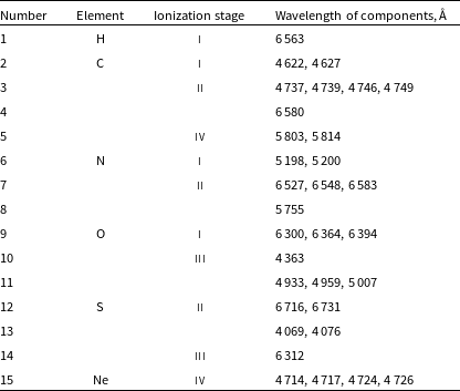
Table 1. Chemical composition of the gas in models. Here
 $n_k$
and
$n_k$
and
 $n_{at}$
– number density of k-th elements’ nuclei and nuclei of all elements respectively.
$n_{at}$
– number density of k-th elements’ nuclei and nuclei of all elements respectively.
In the observed nebulae, a scale of such structures is
 ${\sim} 0.1$
pc. Filaments with a similar distance between them were observed in Tycho supernovae remnant (SNR) (Eriksen et al. Reference Eriksen2011; Laming Reference Laming2015, the last one is an alternative model), or in RX J0852.0-4622 (Pakhomov, Chugai, & Iyudin Reference Pakhomov, Chugai and Iyudin2012). Barkov, Lyutikov, & Khangulyan (Reference Barkov, Lyutikov and Khangulyan2020) propose that this observed structures is produced by variation of density in warm ISM surrounding fast moving pulsars. It must have another origin than filaments in cold molecular clouds. In case of cold ISM, the scale is coincident with the Jeans’ length, but in case of warm ISM with temperature of 10
${\sim} 0.1$
pc. Filaments with a similar distance between them were observed in Tycho supernovae remnant (SNR) (Eriksen et al. Reference Eriksen2011; Laming Reference Laming2015, the last one is an alternative model), or in RX J0852.0-4622 (Pakhomov, Chugai, & Iyudin Reference Pakhomov, Chugai and Iyudin2012). Barkov, Lyutikov, & Khangulyan (Reference Barkov, Lyutikov and Khangulyan2020) propose that this observed structures is produced by variation of density in warm ISM surrounding fast moving pulsars. It must have another origin than filaments in cold molecular clouds. In case of cold ISM, the scale is coincident with the Jeans’ length, but in case of warm ISM with temperature of 10
 $^4$
K, the Jeans’ length is
$^4$
K, the Jeans’ length is
 $\approx$
2 kpc. Consequently, a new process of formation of the structures at the scale 0.1–0.3 pc is required (possibly, a specific regime of thermal instability). Calculation of bow-shock PWNe emissivity maps in many spectral lines could allow us to directly compare the modelling results and observational data.
$\approx$
2 kpc. Consequently, a new process of formation of the structures at the scale 0.1–0.3 pc is required (possibly, a specific regime of thermal instability). Calculation of bow-shock PWNe emissivity maps in many spectral lines could allow us to directly compare the modelling results and observational data.
So far, bow-shock PWNe were systematically observed in
 $\text{H}_\alpha$
line only. The largest survey of 9 objects was carried out by Brownsberger & Romani (Reference Brownsberger and Romani2014). Spectrum of the head part of PSR J2225+6535 nebula (‘Guitar’) only showed hydrogen Balmer series lines (Cordes, Romani, & Lundgren Reference Cordes, Romani and Lundgren1993; Lozinskaya et al. Reference Lozinskaya, Komarova, Moiseev and Blinnikov2005; Danilenko et al. Reference Danilenko, Komarova, Moiseev, Shibanov and Ness2013). However, for the formation of forbidden lines, the neck structures – so-called rings – are expected to be more suitable. These structures are present in many observed PWNe and in favourable conditions could be places of interaction of several shock waves. Such interaction raises density and in consequence the intensity in corresponding lines by a few orders of magnitude. So, the rings could be much brighter in forbidden lines compared to the rest of a nebula. Lines of heavy elements could be even brighter than
$\text{H}_\alpha$
line only. The largest survey of 9 objects was carried out by Brownsberger & Romani (Reference Brownsberger and Romani2014). Spectrum of the head part of PSR J2225+6535 nebula (‘Guitar’) only showed hydrogen Balmer series lines (Cordes, Romani, & Lundgren Reference Cordes, Romani and Lundgren1993; Lozinskaya et al. Reference Lozinskaya, Komarova, Moiseev and Blinnikov2005; Danilenko et al. Reference Danilenko, Komarova, Moiseev, Shibanov and Ness2013). However, for the formation of forbidden lines, the neck structures – so-called rings – are expected to be more suitable. These structures are present in many observed PWNe and in favourable conditions could be places of interaction of several shock waves. Such interaction raises density and in consequence the intensity in corresponding lines by a few orders of magnitude. So, the rings could be much brighter in forbidden lines compared to the rest of a nebula. Lines of heavy elements could be even brighter than
 $\text{H}_\alpha$
.
$\text{H}_\alpha$
.
Barkov, Lyutikov, & Khangulyan (Reference Barkov, Lyutikov and Khangulyan2020) showed that bow shocks of PWNe highlight inhomogeneities of ISM. With successful detection of bow-shock PWNe in various spectral lines, it will be possible to consider a reconstruction of distribution of the density and the chemical composition of the ISM material around the pulsar. It may also shed light on the formation mechanism of ISM inhomogeneities on ultra-low scales.
The aim of the present work is to calculate the synthetic emissivity maps of fast-moving PWNe in
 $\text{H}_\alpha$
and various forbidden spectral lines. We developed a package for the calculation of the intensity maps in spectral lines based on hydrodynamic models accounting for gas ionization state.
$\text{H}_\alpha$
and various forbidden spectral lines. We developed a package for the calculation of the intensity maps in spectral lines based on hydrodynamic models accounting for gas ionization state.
In Section 2, we introduce the methods used for calculating models and synthetic intensity maps. We also give brief description of the relativistic flow morphology. Section 3 is devoted to the visual inspection and the qualitative description of intensity maps. In Section 4, we compare the overall luminosity, morphology and brightness profiles of the synthetic nebulae with the real ones in
 $\text{H}_\alpha$
line. Also, we test scaling laws of nebulae luminosity and put constraints on some dependencies. In Section 5, we give predictions on most suitable lines and physical conditions to observationally explore bow-shock PWNe and highlight the expected features of the morphology with quantitative estimates given. Section 6 is dedicated to the general conclusions.
$\text{H}_\alpha$
line. Also, we test scaling laws of nebulae luminosity and put constraints on some dependencies. In Section 5, we give predictions on most suitable lines and physical conditions to observationally explore bow-shock PWNe and highlight the expected features of the morphology with quantitative estimates given. Section 6 is dedicated to the general conclusions.
2. Methods and models
2.1. Numerical simulation setup
First, 2D relativistic hydrodynamic modelling of pulsar-ISM interaction was performed using the PLUTO codeFootnote a (Mignone et al. Reference Mignone, Bodo, Massaglia, Matsakos, Tesileanu, Zanni and Ferrari2007). In order to simultaneously calculate the hydrodynamic model and calculate the ionization balance of the plasma in the ISM, we used the MINEq module (Tesileanu, Mignone, & Massaglia Reference Tesileanu, Mignone and Massaglia2008). PLUTO is a modular Godunov-type code entirely written in C and intended mainly for astrophysical applications and high Mach number flows in multiple spatial dimensions. In our simulations, we used 3rd order PPM interpolation in space, and 2nd order Runge-Kutta approximation in time with HLLC Riemann solver (Mignone & Bodo Reference Mignone and Bodo2005).
Mixing of ions, ionization, and recombination processes follow the following equation:
 \begin{equation} \partial_t (D X_{k,i}) + \nabla \cdot (D X_{k,i} \mathbf{v}) = D S_{k,i}.\end{equation}
Here, D is a density in the lab frame, k index corresponds to chemical element, i corresponds to the ionization stage, respectively.
 $X_{k,i} \equiv n_{k,i} / n_k$
is the fraction of ions,
$X_{k,i} \equiv n_{k,i} / n_k$
is the fraction of ions,
 $n_{k,i}$
is the number density of the i-th ion of an element k, and
$n_{k,i}$
is the number density of the i-th ion of an element k, and
 $n_{k}$
is the density of the element number.
$n_{k}$
is the density of the element number.
 $S_{k,i}$
is the source term, which accounts for ionization, recombination, and radiative energy losses. The conservative part of equation (1) depicts a transfer of ions and is integrated with hydrodynamic equations.
$S_{k,i}$
is the source term, which accounts for ionization, recombination, and radiative energy losses. The conservative part of equation (1) depicts a transfer of ions and is integrated with hydrodynamic equations.
Only energy density and ionization states are evolving during cooling, so the action of the
 $S_{k,i}$
term is described as a system of ODEs:
$S_{k,i}$
term is described as a system of ODEs:
 \begin{equation} \frac{d}{dt}\binom{E}{X_{k,i}} = \binom{S_E}{S_{k,i}},\end{equation}
where
 $S_E$
is a cooling source term in the energy equation.
$S_E$
is a cooling source term in the energy equation.
Solving the ionization state equations was carried out in the optically-thin plasma limit. The system (2) was integrated as a part of MINEq module apart from hydrodynamics using Runge-Kutta 1-2 method with a switch to Rosenbrock 3-4 if system is stiff and to Cash-Karp 4-5 if estimated error is large. Joint solution with hydrodynamic equations is achieved with Strang splitting, giving a 3rd order precision in spatial coordinates and 2nd in the temporal coordinate.
The chemical composition of the ISM is shown in Table 1. Atomic data were used from Tesileanu, Mignone, & Massaglia (Reference Tesileanu, Mignone and Massaglia2008). For the initial electrons to start ionization MINEq module has a hard-coded floor of
 $10^{-4}$
electron per one nucleus in a cell.
$10^{-4}$
electron per one nucleus in a cell.
Since MINEq module release dielectronic recombination rates have undergone changes, an overview of most recent sources can be found in Laming & Temim (Reference Laming and Temim2020). It would be beneficial to update the data for increase in calculation quality. However, in our setup recombination timescale is much larger than that of ionization (Barkov, Lyutikov, & Khangulyan Reference Barkov, Lyutikov and Khangulyan2020). Overall, it weakly influences dynamics and an the ionization state of gas.
In this setup, we do not account for photoionization from X-ray and ultraviolet radiation from neutron star and PWN itself.
Table 2. Parameters of the grid. Here
 $a=10^{16}$
cm.
$a=10^{16}$
cm.

2.2. Grid parameters
We used a two-dimensional (2D) geometry in cylindrical coordinates. The pulsar is placed in
 $R=0$
and
$R=0$
and
 $z=0$
and the ISM is injected into the computation domain from the left border with speed
$z=0$
and the ISM is injected into the computation domain from the left border with speed
 $V_{NS}$
. The unit of length is
$V_{NS}$
. The unit of length is
 $a = 10^{16}$
cm as in Barkov, Lyutikov, & Khangulyan (Reference Barkov, Lyutikov and Khangulyan2020). The size of the domain is
$a = 10^{16}$
cm as in Barkov, Lyutikov, & Khangulyan (Reference Barkov, Lyutikov and Khangulyan2020). The size of the domain is
 $R \in [0, 35a]$
and
$R \in [0, 35a]$
and
 $z \in [-3a, 100a]$
(
$z \in [-3a, 100a]$
(
 $[-5a, 100a]$
for
$[-5a, 100a]$
for
 $V_{NS}=150\,\text{km/s}$
). To have a good resolution in the central region and the long tail zone, we use a non-uniform resolution in the computational domain with the total number of cells
$V_{NS}=150\,\text{km/s}$
). To have a good resolution in the central region and the long tail zone, we use a non-uniform resolution in the computational domain with the total number of cells
 $N_\textrm{R} = 520$
, and
$N_\textrm{R} = 520$
, and
 $N_\textrm{z} = 1\,560$
(
$N_\textrm{z} = 1\,560$
(
 $1\,690$
for
$1\,690$
for
 $V_{NS}=150\,\text{km/s}$
). See more details in Table 2. The simulations were performed on CFCA XC50 cluster of National Astronomical Observatory of Japan (NAOJ).
$V_{NS}=150\,\text{km/s}$
). See more details in Table 2. The simulations were performed on CFCA XC50 cluster of National Astronomical Observatory of Japan (NAOJ).
2.3. Initial and boundary conditions
Initial and boundary conditions are as follows:
-
• ISM injection zone.
Velocity of the cold (
 $p \ll \rho v^2$
) gas flow:
$(0;\,V_{NS})$
. Cases: (3)
\begin{equation} V_{NS}=150,\,450,\,1\,500\,\text{km/s}. \end{equation}
$p \ll \rho v^2$
) gas flow:
$(0;\,V_{NS})$
. Cases: (3)
\begin{equation} V_{NS}=150,\,450,\,1\,500\,\text{km/s}. \end{equation}
ISM density varies in order to simulate the so-called ‘shoulder-neck’ structures in nebulae following the equation:
(4)where
\begin{equation} \rho_{ISM} = \frac{\rho_0}{1-a_\rho \sin \left[ \frac{z-t V_{NS}}{\lambda}\right]}, \end{equation}
$\rho_0=m_p/\text{cm}^3$
,
$\lambda = 30 \times 10^{16}$
cm – length scale of
$\rho_{ISM}$
fluctuations,
$a_\rho = 0.5$
– their amplitude. Equilibrium ionization state.
For
$V_{NS}=150\,\text{km/s}$
, the ISM density is constant and set to
$\rho_0$
. -
• Internal boundary condition (pulsar wind ejection zone). We inject the spherically isotropic cold wind:
$p / \rho c^2 = 1 / 100$
(which correspond to Mach number
$M=42$
), and Lorentz factor is
$\Gamma = 4.9$
. Stand-off distance (see Barkov, Lyutikov, & Khangulyan Reference Barkov, Lyutikov and Khangulyan2019 for details) is
$r_s = 0.57 \times 10^{16}$
cm. -
• Other boundary conditions are the following: wind outflow at the tail side of nebula, axisymmetric/fully reflective boundary conditions at central axis, free outflow on outer boundary.
-
• For different models (see Table 3) we used the ideal equation of state with two values of the adiabatic index
(5)For
\begin{equation}\gamma = \frac{4}{3}, \frac{5}{3}.\end{equation}
$V_{NS}=150\,\text{km/s}$
only
$\gamma = 4/3$
is considered.


All names of the models are listed in Table 3:
Table 3. Parameters of the models.

2.4. Method of emissivity calculation
In order to calculate emissivity maps, a high-performance program package was created. We called it Shu (Nikonorov Reference Nikonorov2023) after the Egyptian god of the air and supporter of the sky. His ostrich feather was symbolic of lightness and emptiness. Shu was considered to be a cooling, and thus calming, influence, and a pacifier.
The package uses all resources of a workstation, such as CPU, GPU and fast SSD storage. The structural scheme of the package is shown in Figure 1.
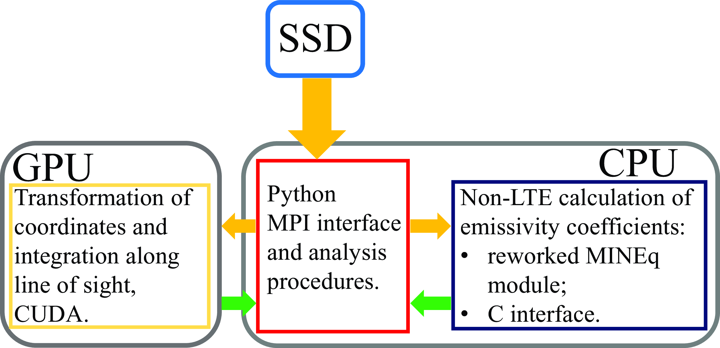
Figure 1. Block-scheme of Shu package. Yellow arrows show inputs of processes, green ones show outputs.
Reading hydrodynamic simulation checkpoints is done in the Python-runtime processes with the PyPLUTO package. Parallelism is implemented on simulation checkpoints using MPI. RAM addresses of the data are being transferred to the C-module based on MINEq. The major difference between modules is that MINEq calculates cooling function in the unit of volume, whereas our module calculates an emissivity coefficient:
 \begin{align} MINEq\ {:}\ S_E & = - \left( n_{at} n_e \Lambda (T, \mathbf{X}) +L_{FF} +L_{I-R} \right),\end{align}
 \begin{align}\text{Our work}\ {:}\ \eta_{em} & = n_{at} n_e \hat{\Lambda} (T, X_{k,i}) / 4 \pi, \end{align}
where
 $\Lambda$
is the part of a cooling function due to cooling in spectral lines, normalised to the concentration of electrons and ions;
$\Lambda$
is the part of a cooling function due to cooling in spectral lines, normalised to the concentration of electrons and ions;
 $\hat{\Lambda}$
– its part due to lines, which were selected for calculation;
$\hat{\Lambda}$
– its part due to lines, which were selected for calculation;
 $X_{k,i}$
– the part of i-th ion among all of k-th element atoms;
$X_{k,i}$
– the part of i-th ion among all of k-th element atoms;
 $\mathbf{X}$
is the gas ionization state.
$\mathbf{X}$
is the gas ionization state.
After that, arrays of emissivity coefficients are being sent to VRAM by MPI processes. On GPU, a conversion from the non-uniform 2D grid to the uniform 3D grid and the summation along the line of sight takes place. The conversion is carried out by the coordinate system rotation and the nearest-neighbour interpolation. Parallelism here is based on the breaking down calculation task to compute individual pixels of the intensity map (about
 $8\times10^5$
pixels per map, which is much more than number of CUDA cores in one GPU).
$8\times10^5$
pixels per map, which is much more than number of CUDA cores in one GPU).
Atoms and ions available for calculation are H, He and their ions, five lowest ionization stages of C, N, O, Ne and S – 23 species in total. Electron configurations vary from those of hydrogen-like elements (
 $1s^1$
), alkali metals (
$1s^1$
), alkali metals (
 $2s^1$
), helium-like elements (
$2s^1$
), helium-like elements (
 $1s^2$
) and alkaline earth metals (
$1s^2$
) and alkaline earth metals (
 $n s^2$
) to elements with 1–6 p electrons (
$n s^2$
) to elements with 1–6 p electrons (
 $n p^1$
–
$n p^1$
–
 $n p^6$
). The detailed description of the given configurations’ spectra can be found in Sobelman (Reference Sobelman1979). The considered configuration belongs to elements in various ionization stages, generating many emission lines from the ultraviolet to infrared spectral range. At the moment, only configurations with d and f electrons are not available for computation, as well as the fifth ionization stage, in which an excess of population occurs because of the lack of higher stages.
$n p^6$
). The detailed description of the given configurations’ spectra can be found in Sobelman (Reference Sobelman1979). The considered configuration belongs to elements in various ionization stages, generating many emission lines from the ultraviolet to infrared spectral range. At the moment, only configurations with d and f electrons are not available for computation, as well as the fifth ionization stage, in which an excess of population occurs because of the lack of higher stages.
We studied all optical lines available for the calculation given a restriction of low energy level count in models of ions (usually 3–10 levels including a fine structure), except helium (we plan to upgrade models of H and He atoms and ion and make research on them in a separate work). The goal was to determine which of the factors impact expected observational features of bow-shock PWNe the most. Thus, besides H i, species with configurations of alkali metals (C iv), alkaline-earth metals (C iii),
 $n p^1$
(C ii),
$n p^1$
(C ii),
 $n p^2$
(C i, N ii, O iii, S iii),
$n p^2$
(C i, N ii, O iii, S iii),
 $n p^3$
(N i, S ii, Ne iv), and
$n p^3$
(N i, S ii, Ne iv), and
 $n p^4$
(O i) were chosen for the analysis. Also, [O iii], [S ii], [N ii] and [O i] lines are the most common to research extended objects. The list of lines is presented in Table 4.
$n p^4$
(O i) were chosen for the analysis. Also, [O iii], [S ii], [N ii] and [O i] lines are the most common to research extended objects. The list of lines is presented in Table 4.
Table 4. List of lines and multiplets, in which intensity maps are calculated in this work.
We upgraded a model of C iv (to 24 levels). We used effective collision strengths from Aggarwal & Keenan (Reference Aggarwal and Keenan2004) and radiative transitions data from Chianti v10.1 (Del Zanna et al. Reference Del Zanna, Dere, Young and Landi2021). Extension of the model allowed us to study more spectral lines. In the future, extension of H and He atoms and ion models will be useful.
2.5. Calculated models
In every model, we obtained an equilibrium quasi-stationary solution. Density maps and flow streamlines are shown in Figures 2 and 3.
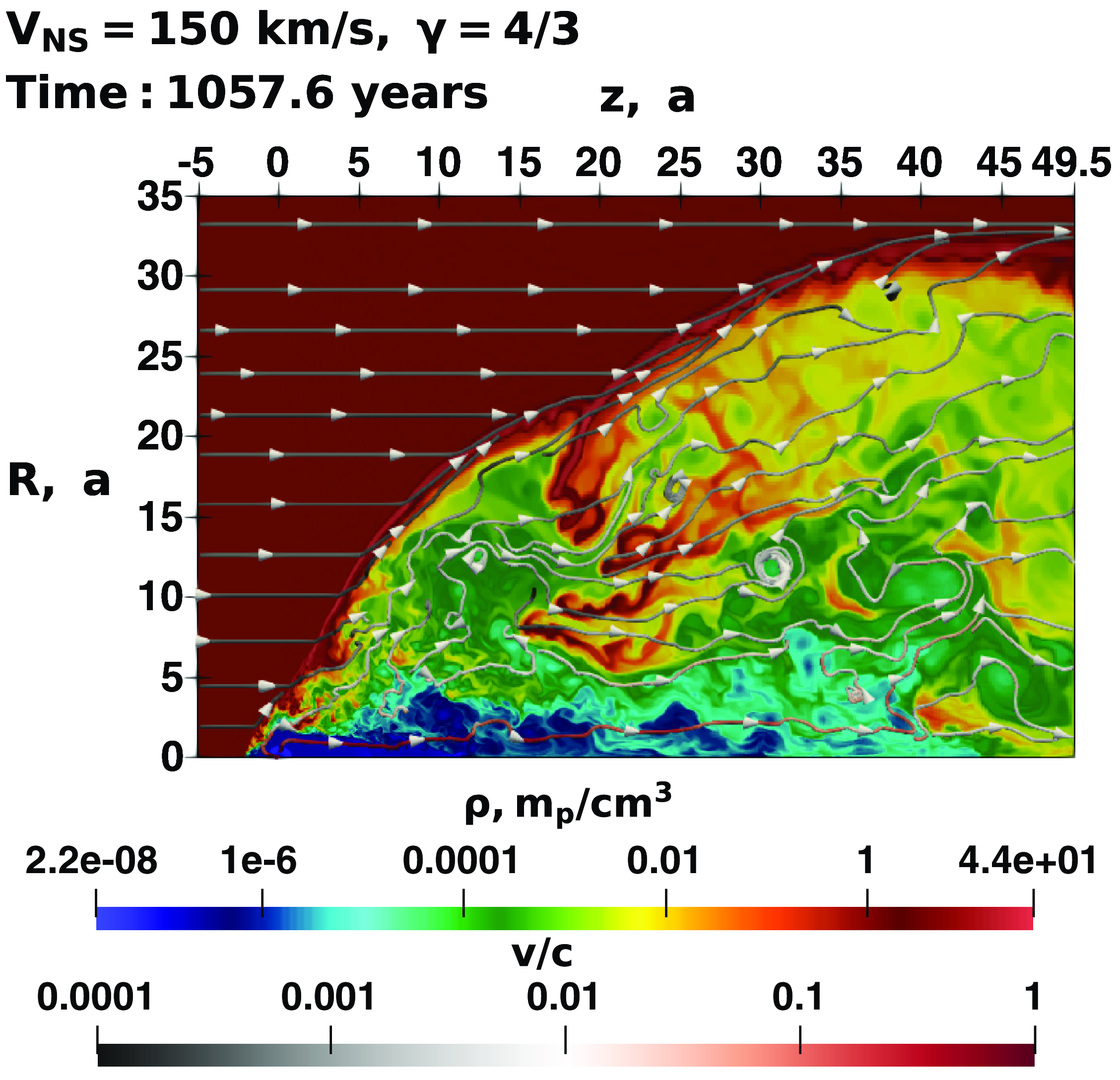
Figure 2. Distribution of density and velocity in pulsar frame of reference in v01g43nv model. The logarithm of density in
 $m_p / \text{cm}^3$
is shown by colour. The velocity field is shown with streamlines with arrows.
$m_p / \text{cm}^3$
is shown by colour. The velocity field is shown with streamlines with arrows.

Figure 3. Same, as Figure 2, for v03g43, v03g53, v1g43 and v1g53 models.
There is a forward shock on the outer part of the nebula (crimson colour on Figures 2 and 3), on which neutral ISM is shocked and compressed. A zone of shocked ISM is spanning inwards untill a contact discontinuity (mostly yellow-green colour), which is present on the head of the nebula at
 $V_{NS} = 450$
km/s. Then due to strong mixing it breaks down via Kelvin-Helmholtz instability. At
$V_{NS} = 450$
km/s. Then due to strong mixing it breaks down via Kelvin-Helmholtz instability. At
 $V_{NS} = 1\,500$
km/s a contact discontinuity remains intact not only on the head, but on a following bubble, even though with some mixing. In the tail of the nebula there is a vast zone of shocked pulsar wind mixed with ISM (yellow and green colours). At the inner part of the shocked wind zone, on the boundary with an unshocked wind (dark blue colour), a reverse shock with a Mach disk is formed (a jump in density, depicted as jump in colour). It is located near the position of the pulasr:
$V_{NS} = 1\,500$
km/s a contact discontinuity remains intact not only on the head, but on a following bubble, even though with some mixing. In the tail of the nebula there is a vast zone of shocked pulsar wind mixed with ISM (yellow and green colours). At the inner part of the shocked wind zone, on the boundary with an unshocked wind (dark blue colour), a reverse shock with a Mach disk is formed (a jump in density, depicted as jump in colour). It is located near the position of the pulasr:
 $(R, z) = (0, 0)$
.
$(R, z) = (0, 0)$
.
The main factor impacting the nebula morphology is the pulsar velocity. For the value 450 km/s, the interaction with the perturbations in the ISM is relatively long and distinctive, so-called bubbles are forming in the tail of the nebula. When the pulsar passes a region with low ISM density, the bow shock starts almost isotropic expansion and forms a close to spherical bubble in the tale of the nebula. In the high density region, the shock wave propagates slower, forming a so-called neck zone. At high pulsar velocity
 $1\,500$
km/s, bubbles are characterised by a notably smaller size. In the high velocity case, we see less prominent mixing of shocked ISM matter with pulsar wind one.
$1\,500$
km/s, bubbles are characterised by a notably smaller size. In the high velocity case, we see less prominent mixing of shocked ISM matter with pulsar wind one.
Another kind of features presented in our models and also observed by Brownsberger & Romani (Reference Brownsberger and Romani2014) in some objects is formation of so-called rings, where shocks of two bubbles collide. In the area of the collision, the density of the matter grows rapidly and can reach the value
 ${\sim}$
80
${\sim}$
80
 $m_p/$
cm
$m_p/$
cm
 $^3$
, and the number density of electrons can be as high as
$^3$
, and the number density of electrons can be as high as
 ${\sim}$
40
${\sim}$
40
 $/$
cm
$/$
cm
 $^3$
. The temperature is not as high (falls to a hundred thousands K) as in other shocked regions. Taking into account low matter density and short dynamical timescale, these conditions favour a low ionization stages of atoms.
$^3$
. The temperature is not as high (falls to a hundred thousands K) as in other shocked regions. Taking into account low matter density and short dynamical timescale, these conditions favour a low ionization stages of atoms.
The solution varies noticeably with the adiabatic index (
 $\gamma$
) of the ideal gas. The distinction between values is in the compression ratio in strong shocks, which is equal to 7 for
$\gamma$
) of the ideal gas. The distinction between values is in the compression ratio in strong shocks, which is equal to 7 for
 $\gamma$
= 4/3 and 4 for
$\gamma$
= 4/3 and 4 for
 $\gamma$
= 5/3. The first case is the ultrarelativistic limit for the adiabatic index, which is applicable to strongly relativistic flows. However, it results in density behind shocks being overestimated by almost a factor of 2. The last case is the classical limit that is applicable to shocks in the ISM. But relativistic winds‘ ability to compress becomes underestimated, that leads to intensive mixing with ISM. Thus, the overall morphology of the nebula is better described in case of
$\gamma$
= 5/3. The first case is the ultrarelativistic limit for the adiabatic index, which is applicable to strongly relativistic flows. However, it results in density behind shocks being overestimated by almost a factor of 2. The last case is the classical limit that is applicable to shocks in the ISM. But relativistic winds‘ ability to compress becomes underestimated, that leads to intensive mixing with ISM. Thus, the overall morphology of the nebula is better described in case of
 $\gamma$
= 4/3, but shocks in ISM, which are essential for calculating the emissivity, are more realistic in case of
$\gamma$
= 4/3, but shocks in ISM, which are essential for calculating the emissivity, are more realistic in case of
 $\gamma$
= 5/3. In reality, one can expect behaviour in between of these cases.
$\gamma$
= 5/3. In reality, one can expect behaviour in between of these cases.
Direct comparison of flow morphology in the low speed model (
 $V_{NS}=$
150 km/s) with high velocity models is not straightforward due to initial uniform density of ISM, as shown in Table 3. Also, due to low pulsar speed and fast expansion of the bow shock in radial direction, the morphology of the nebula in this case only developed in
$V_{NS}=$
150 km/s) with high velocity models is not straightforward due to initial uniform density of ISM, as shown in Table 3. Also, due to low pulsar speed and fast expansion of the bow shock in radial direction, the morphology of the nebula in this case only developed in
 $z\lt$
50 a region. Further simulation was meaningless; Mach cone leaves the computation domain. Nevertheless, we are able to highlight some distinct features of the model. The interaction of pulsar wind with ISM is the most active and strong. Due to Kelvin-Helmholtz instability, ISM matter actively mixes with pulsar wind, forming a complex and dynamic inner structure of nebula.
$z\lt$
50 a region. Further simulation was meaningless; Mach cone leaves the computation domain. Nevertheless, we are able to highlight some distinct features of the model. The interaction of pulsar wind with ISM is the most active and strong. Due to Kelvin-Helmholtz instability, ISM matter actively mixes with pulsar wind, forming a complex and dynamic inner structure of nebula.
3. Synthetic intensity maps
In the case of intensity maps appears a new free parameter
 $\chi$
– angle between
$\chi$
– angle between
 $V_{NS}$
and picture plane. How intensity maps react to the variation of
$V_{NS}$
and picture plane. How intensity maps react to the variation of
 $\chi$
was investigated in the paper (Barkov, Lyutikov, & Khangulyan Reference Barkov, Lyutikov and Khangulyan2020). Here we calculated intensity maps of fast moving pulsar nebulae in various spectral lines for
$\chi$
was investigated in the paper (Barkov, Lyutikov, & Khangulyan Reference Barkov, Lyutikov and Khangulyan2020). Here we calculated intensity maps of fast moving pulsar nebulae in various spectral lines for
 $\chi=0.2$
rad. We present mapped values of intensity, which are unchanged with varying distance to the object if the extinction is not significant. Angular size of nebula can vary, so we plot intensity against physical size. The coordinates of intensity maps are (X, Y), their plane is rotated by
$\chi=0.2$
rad. We present mapped values of intensity, which are unchanged with varying distance to the object if the extinction is not significant. Angular size of nebula can vary, so we plot intensity against physical size. The coordinates of intensity maps are (X, Y), their plane is rotated by
 $\chi$
around R (or X) axis with respect to (R, z), similar to Barkov, Lyutikov, & Khangulyan (Reference Barkov, Lyutikov and Khangulyan2020).
$\chi$
around R (or X) axis with respect to (R, z), similar to Barkov, Lyutikov, & Khangulyan (Reference Barkov, Lyutikov and Khangulyan2020).
The maps are presented in Figures 4–8 and share some common features. Firstly, emitting regions has a layered structure, with a layer having a surface and near-certain depth (smoothness of emitting layers on presented maps is partly due to 2D calculations).

Figure 4. Synthetic intensity map of model v01g43nv nebula in
 $\text{H}_\alpha$
. The contours highlight levels 1 (olive colour), 3 (dark khaki) and 10
$\text{H}_\alpha$
. The contours highlight levels 1 (olive colour), 3 (dark khaki) and 10
 $I_{17}$
(gold); here
$I_{17}$
(gold); here
 $I_{17} = 10^{-17}\frac{\text{erg}}{\text{s} \times \text{cm}^2 \times \text{arcsec}^2}.$

Figure 5. Same, as Figure 4, for v03g43 (top left panel), v03g53 (top right panel), v1g43 (bottom left panel) and v1g53 (bottom right panel) models.

Figure 6. Synthetic intensity maps in the brightest optical lines of neutral atoms in calculation: [N i]
 $\lambda\lambda$
5 198, 5 200 Å (left panel), [O i]
$\lambda\lambda$
5 198, 5 200 Å (left panel), [O i]
 $\lambda\lambda$
6 300, 6 364, 6 394 Å (right panel). Contours highlight 1, 3 and 10
$\lambda\lambda$
6 300, 6 364, 6 394 Å (right panel). Contours highlight 1, 3 and 10
 $I_{17}$
.
$I_{17}$
.

Figure 7. Synthetic intensity maps in the brightest optical lines of singly ionized atoms in calculation: [N ii]
 $\lambda\lambda$
6 527, 6 548, 6 583 Å (left panel), [S ii]
$\lambda\lambda$
6 527, 6 548, 6 583 Å (left panel), [S ii]
 $\lambda\lambda$
6 716, 6 731 Å (right panel). Contours highlight 1, 3 and 10
$\lambda\lambda$
6 716, 6 731 Å (right panel). Contours highlight 1, 3 and 10
 $I_{17}$
.
$I_{17}$
.
By the reason of projection effect, nebulae are much brighter to the edges of bubbles – a bulk of emitting material lies on the line of sight there. This is shown by contours on intensity maps, which represent typical values for detection of extended emission on relatively low signal level (we assume a typical value of
 $10^{-17}\frac{\text{erg}}{\text{s} \times \text{cm}^2 \times \text{arcsec}^2}$
, olive colour); higher signal levels
$10^{-17}\frac{\text{erg}}{\text{s} \times \text{cm}^2 \times \text{arcsec}^2}$
, olive colour); higher signal levels
 $3\times10^{-17}$
and
$3\times10^{-17}$
and
 $10^{-16}\frac{\text{erg}}{\text{s} \times \text{cm}^2 \times \text{arcsec}^2}$
are indicated by dark khaki and gold colours, respectively. Those values are shared by the contours in all the figures presented.
$10^{-16}\frac{\text{erg}}{\text{s} \times \text{cm}^2 \times \text{arcsec}^2}$
are indicated by dark khaki and gold colours, respectively. Those values are shared by the contours in all the figures presented.
3.1. Emission maps in lines of neutral atoms
 $\text{H}_\alpha$
is the most important line for research of bow-shock PWNe. Now, it is the only line in which these objects are systematically observed and can be directly compared with numerical models (see Barkov, Lyutikov, & Khangulyan Reference Barkov, Lyutikov and Khangulyan2020). Furthermore, it is quite useful as a standard for analysis of other spectral lines and a marker of modern observational possibilities. Therefore, we calculated intensity maps for it first. They are presented on Figures 4 and 5. We also performed comparison with observations, which is described in Section 4.1.
$\text{H}_\alpha$
is the most important line for research of bow-shock PWNe. Now, it is the only line in which these objects are systematically observed and can be directly compared with numerical models (see Barkov, Lyutikov, & Khangulyan Reference Barkov, Lyutikov and Khangulyan2020). Furthermore, it is quite useful as a standard for analysis of other spectral lines and a marker of modern observational possibilities. Therefore, we calculated intensity maps for it first. They are presented on Figures 4 and 5. We also performed comparison with observations, which is described in Section 4.1.
Only a thin layer of ISM matter just behind the bow shock emits in
 $\text{H}_\alpha$
, since H i exists only in low temperature plasma and maximum emissivity is achieved around X(H i)
$\text{H}_\alpha$
, since H i exists only in low temperature plasma and maximum emissivity is achieved around X(H i)
 $\approx$
0.5. It is being reached by collisions with energetic electrons in short after ISM matter passes the bow shock (
$\approx$
0.5. It is being reached by collisions with energetic electrons in short after ISM matter passes the bow shock (
 ${\sim} 5$
cells). On the one hand, this feature allows an easy detection with observations and a direct study of the environment near bow shock. But on the other,
${\sim} 5$
cells). On the one hand, this feature allows an easy detection with observations and a direct study of the environment near bow shock. But on the other,
 $\text{H}_\alpha$
photons are not being emitted from deeper regions of the nebula. It makes gathering information about deep volume structure in this waveband impossible, and observations in other lines become highly demanded.
$\text{H}_\alpha$
photons are not being emitted from deeper regions of the nebula. It makes gathering information about deep volume structure in this waveband impossible, and observations in other lines become highly demanded.
Other bright lines of neutral atoms are [N i]
 $\lambda\lambda$
5 198, 5 200 Å doublet and [O i]
$\lambda\lambda$
5 198, 5 200 Å doublet and [O i]
 $\lambda\lambda$
6 300, 6 364, 6 394 Å triplet with the 6 300 Å brightest component (synthetic intensity maps are presented in Figure 6). These lines mostly highlight the same features as
$\lambda\lambda$
6 300, 6 364, 6 394 Å triplet with the 6 300 Å brightest component (synthetic intensity maps are presented in Figure 6). These lines mostly highlight the same features as
 $\text{H}_\alpha$
and highlight the bow shock of the nebula. We see a less uniform intensity distribution, with slight humps on the front and back parts of the bubbles. The other difference is that, unlike
$\text{H}_\alpha$
and highlight the bow shock of the nebula. We see a less uniform intensity distribution, with slight humps on the front and back parts of the bubbles. The other difference is that, unlike
 $\text{H}_\alpha$
, centres of bubbles have lower intensity and rings become visible.
$\text{H}_\alpha$
, centres of bubbles have lower intensity and rings become visible.
3.2. Emission maps in lines of singly ionized atoms
The brightest lines of singly ionized atoms are [N ii]
 $\lambda\lambda$
6 527, 6 548, 6 583 Å nebular triplet and [S ii]
$\lambda\lambda$
6 527, 6 548, 6 583 Å nebular triplet and [S ii]
 $\lambda\lambda$
6 716, 6 731 Å doublet. Synthetic intensity maps of them are shown in Figure 7. Spectral lines of atoms in the second ionization stage are placed on the intermediate depth relatively to shock front. Emission comes from a thin layer at bow shock, the head of nebula is dimmer and rings are brighter than in the case of neutral atoms. Regions of rings stand out due to high density and relatively low temperature. Thickness of the rings are
$\lambda\lambda$
6 716, 6 731 Å doublet. Synthetic intensity maps of them are shown in Figure 7. Spectral lines of atoms in the second ionization stage are placed on the intermediate depth relatively to shock front. Emission comes from a thin layer at bow shock, the head of nebula is dimmer and rings are brighter than in the case of neutral atoms. Regions of rings stand out due to high density and relatively low temperature. Thickness of the rings are
 ${\sim} 2a$
with
${\sim} 2a$
with
 $T\lt40\,000$
K in v03g43 model, density reaches
$T\lt40\,000$
K in v03g43 model, density reaches
 $\gtrsim 10\,m_p/\text{cm}^3$
.
$\gtrsim 10\,m_p/\text{cm}^3$
.
In v03 models, regions of line formation start shifting to rings, although their inner structure is only slightly noticeable. Bow shock is strongly expressed. In v01g43nv model the same features appear, but bright filaments are formed from ISM matter as a product of turbulence in shocked pulsar wind.

Figure 8. Synthetic intensity maps in the brightest optical lines of doubly ionized atoms in calculation: [O iii]
 $\lambda\lambda$
4 933, 4 959, 5 007 Å. Contours highlight 1, 3 and 10
$\lambda\lambda$
4 933, 4 959, 5 007 Å. Contours highlight 1, 3 and 10
 $I_{17}$
.
$I_{17}$
.
3.3. Emission maps in lines of doubly ionized atoms
The [O iii]
 $\lambda\lambda$
4 933, 4 959, 5 007 Å triplet is the most bright lines of twice ionized atoms. Synthetic intensity maps of it are shown in Figure 8. O iii ions and thus their emission exists in a thick layer of a favourable temperature regime. They form rings, which are more pronounced than rings in other lines. Its emission zone lays deep behind the bow shock on the intensity maps. The cross-section radius of nebula bubbles is smaller than in
$\lambda\lambda$
4 933, 4 959, 5 007 Å triplet is the most bright lines of twice ionized atoms. Synthetic intensity maps of it are shown in Figure 8. O iii ions and thus their emission exists in a thick layer of a favourable temperature regime. They form rings, which are more pronounced than rings in other lines. Its emission zone lays deep behind the bow shock on the intensity maps. The cross-section radius of nebula bubbles is smaller than in
 $\text{H}_\alpha$
. Features mentioned above make observations and detection in [O iii] easier due to high contrast. The diffuse background emission of ISM is smaller in the case of [O iii] triplet than in
$\text{H}_\alpha$
. Features mentioned above make observations and detection in [O iii] easier due to high contrast. The diffuse background emission of ISM is smaller in the case of [O iii] triplet than in
 $\text{H}_\alpha$
.
$\text{H}_\alpha$
.
4. Comparison between observations and models for
$\text{H}_\alpha$

4.1. Scaling flux of observed objects using ATNF radio data
For verification of our results, we compare integrated flux of the models and observed flux in
 $\text{H}_\alpha$
line for 7 nebulae. We take into account integrated fluxes, extinction in R-band (Brownsberger & Romani Reference Brownsberger and Romani2014), and spin-down power, proper motion velocity, and distances from Australia Telescope National Facility catalogue version 1.70 (ATNF, see Manchester et al. Reference Manchester, Hobbs, Teoh and Hobbs2005).
$\text{H}_\alpha$
line for 7 nebulae. We take into account integrated fluxes, extinction in R-band (Brownsberger & Romani Reference Brownsberger and Romani2014), and spin-down power, proper motion velocity, and distances from Australia Telescope National Facility catalogue version 1.70 (ATNF, see Manchester et al. Reference Manchester, Hobbs, Teoh and Hobbs2005).
We calculate PWNe luminosity as:
 \begin{equation} L _{\text{H}\alpha} = F_{T, \text{H}\alpha} \frac{h c}{\lambda_{\text{H}\alpha}} 4 \pi D^2\,10^{0.4 A_R},\end{equation}
where
 $F_{T, \text{H}\alpha}$
– observed integrated
$F_{T, \text{H}\alpha}$
– observed integrated
 $\text{H}_\alpha$
flux in cm
$\text{H}_\alpha$
flux in cm
 $^{-2}\textit{s}^{-1}$
, h – Plank’s constant, c – speed of light,
$^{-2}\textit{s}^{-1}$
, h – Plank’s constant, c – speed of light,
 $\lambda_{\text{H}\alpha}$
–
$\lambda_{\text{H}\alpha}$
–
 $\text{H}_\alpha$
wavelength (6 563 Å), D – distance to pulsar,
$\text{H}_\alpha$
wavelength (6 563 Å), D – distance to pulsar,
 $A_R$
– extinction in red waveband.
$A_R$
– extinction in red waveband.
For most PWNe, the pulsar speed is measured only in the plane of the sky (
 $V_\tau$
). Assuming a general population of pulsars’ velocity is being isotropically distributed in space, and their local ISM is at rest in respect to the Galactic rotation (Manchester et al. Reference Manchester, Hobbs, Teoh and Hobbs2005, give detailed description of determining
$V_\tau$
). Assuming a general population of pulsars’ velocity is being isotropically distributed in space, and their local ISM is at rest in respect to the Galactic rotation (Manchester et al. Reference Manchester, Hobbs, Teoh and Hobbs2005, give detailed description of determining
 $V_\tau$
), we can calculate spatial velocities relative to the local ISM as:
$V_\tau$
), we can calculate spatial velocities relative to the local ISM as:
 \begin{equation} V_{NS} = \sqrt{3/2} V_\tau.\end{equation}
The parameters of bow-shock PWNe, which were defined from optical observations (Brownsberger & Romani Reference Brownsberger and Romani2014), strongly correlate with each other (for example, the flux from the nebula’s head and its size are practically linearly dependent on log – log scale). It could be caused by natural reasons as selection effects of observations. At the moment, we cannot distinguish the true nature of the observed correlation. We use only data from radio wavelengths in order to calibrate luminosity. Independent data sources are highly demanded.
Properties of the observed nebulae vary and don’t coincide with models’ parameters. This fact requires the development of a calibration procedure, which can be applied to the bow-shock PWNe. In the Appendix A we discussed various procedures of the calibration. Finally, we attained an equation for
 $\text{H}_\alpha$
luminosity as:
$\text{H}_\alpha$
luminosity as:
 \begin{equation} L_{\text{H}\alpha}^{calibrated} (V_{NS}) = L_{\text{H}\alpha} \dot{E}_{model}(V_{NS}) / \dot{E}.\end{equation}
Here
 $\dot{E}_{model}$
– spin-down power of model pulsar. This quantity corresponds to model
$\dot{E}_{model}$
– spin-down power of model pulsar. This quantity corresponds to model
 $\rho_{ISM} = 1\,m_p/\text{cm}^3$
and
$\rho_{ISM} = 1\,m_p/\text{cm}^3$
and
 $r_s = 0.57$
a, and given
$r_s = 0.57$
a, and given
 $V_{NS}$
, according to equation (A5).
$V_{NS}$
, according to equation (A5).
In Figure 9, we present the comparison of
 $\text{H}_\alpha$
luminosity versus pulsar velocity between model and observed nebulae. Most values are close to models with
$\text{H}_\alpha$
luminosity versus pulsar velocity between model and observed nebulae. Most values are close to models with
 $\gamma=4/3$
and
$\gamma=4/3$
and
 $\max(z) = 49.5$
a. The models are consistent with the observational data. The consistency is present throughout different methods of measuring the distance to pulsars, which strongly affects the luminosity estimation.
$\max(z) = 49.5$
a. The models are consistent with the observational data. The consistency is present throughout different methods of measuring the distance to pulsars, which strongly affects the luminosity estimation.
Nebula of PSR J0437-4715 shows 0.5 orders less luminous than others. It has the largest stand-off angular distance (9”) of all observed nebulae, so we presume that lacking luminosity may belong to regions outside the telescopes’ field of view. There may be the case analogous to nebula of PSR J0742-2822, described by Brownsberger & Romani (Reference Brownsberger and Romani2014), when past observations detected nebula’s front part with high surface brightness, and following ones discovered a tail having lower surface brightness, but due to its size giving noticeable contribution to overall nebula’s flux in
 $\text{H}_\alpha$
. We also cannot fully exclude the hypothesis of pre-ionization by non-thermal emission, due to which ISM material is partially ionized before passing bow shock. The possibility of this scenario was discussed in Cordes, Romani, & Lundgren (Reference Cordes, Romani and Lundgren1993), Chatterjee & Cordes (Reference Chatterjee and Cordes2002), Brownsberger & Romani (Reference Brownsberger and Romani2014).
$\text{H}_\alpha$
. We also cannot fully exclude the hypothesis of pre-ionization by non-thermal emission, due to which ISM material is partially ionized before passing bow shock. The possibility of this scenario was discussed in Cordes, Romani, & Lundgren (Reference Cordes, Romani and Lundgren1993), Chatterjee & Cordes (Reference Chatterjee and Cordes2002), Brownsberger & Romani (Reference Brownsberger and Romani2014).
Nebulae of PSR J1856-3754 and PSR J2225+6535 were excluded from the comparison. For the first one, there is a possibility of it being the photoionization nebula, which was discussed by van Kerkwijk & Kulkarni (Reference van Kerkwijk and Kulkarni2001). In the second case, Chatterjee & Cordes (Reference Chatterjee and Cordes2002) measured atypically low stand-off angle (
 ${\sim} 0.1$
”). Explanation of its value is challenging, especially considering the nebula’s long and bright tail. In both cases, further research is required.
${\sim} 0.1$
”). Explanation of its value is challenging, especially considering the nebula’s long and bright tail. In both cases, further research is required.
Considering dependency of luminosity from pulsar speed, we notice
 $L_{\text{H}\alpha}$
being approximately constant throughout the entire range of pulsar velocity in the set of models with
$L_{\text{H}\alpha}$
being approximately constant throughout the entire range of pulsar velocity in the set of models with
 $\max(z) = 49.5$
a, which is closest to observations. In the same time, in our models, the spin-down power is proportional to the pulsar velocity squared. And due to equation (A12), in order for
$\max(z) = 49.5$
a, which is closest to observations. In the same time, in our models, the spin-down power is proportional to the pulsar velocity squared. And due to equation (A12), in order for
 $L_{\text{H}\alpha}$
to be constant, there must be limitation on
$L_{\text{H}\alpha}$
to be constant, there must be limitation on
 $f(V_{NS})$
and its components (see Appendix A for the details):
$f(V_{NS})$
and its components (see Appendix A for the details):
 \begin{align} \dot{E}_{model} \propto V_{NS}^2,\end{align}
 \begin{align} f(V_{NS}) &\propto V_{NS}^{-2},\end{align}
 \begin{align} \epsilon_{\text{H}\alpha} \eta^2 &\propto V_{NS}^{-1}.\end{align}
If
 $\epsilon_{\text{H}\alpha}$
is approximately independent of the pulsar velocity (equation A1), then the coefficient
$\epsilon_{\text{H}\alpha}$
is approximately independent of the pulsar velocity (equation A1), then the coefficient
 $\eta \propto V_{NS}^{-\frac{1}{2}}$
. This contradicts Chatterjee & Cordes (Reference Chatterjee and Cordes2002), but seems plausible, because nebula cone shrinks with increase of pulsar velocity.
$\eta \propto V_{NS}^{-\frac{1}{2}}$
. This contradicts Chatterjee & Cordes (Reference Chatterjee and Cordes2002), but seems plausible, because nebula cone shrinks with increase of pulsar velocity.
If
 $\epsilon_{\text{H}\alpha}$
is proportional to the pulsar velocity in the negative power law,
$\epsilon_{\text{H}\alpha}$
is proportional to the pulsar velocity in the negative power law,
 $\eta$
is less defendant in the pulsar velocity. For equations (A2) and (A3), there is
$\eta$
is less defendant in the pulsar velocity. For equations (A2) and (A3), there is
 $\eta \propto V_{NS}^{-\frac{1}{4}}$
and
$\eta \propto V_{NS}^{-\frac{1}{4}}$
and
 $\eta \propto V_{NS}^{-\frac{1}{8}}$
respectively. This also seems plausible and more consistent with Chatterjee & Cordes (Reference Chatterjee and Cordes2002).
$\eta \propto V_{NS}^{-\frac{1}{8}}$
respectively. This also seems plausible and more consistent with Chatterjee & Cordes (Reference Chatterjee and Cordes2002).
4.2. Morphology comparison
An important criterion of models’ correctness is consistency between model and observed nebulae morphology. We compare the nebula PSR J0742-2822 and the model v03g43 profiles in the
 $\text{H}_\alpha$
line. This object was selected due to long tail region and probable proximity of pulsar velocity to picture plane. Observational data was taken from Brownsberger & Romani (Reference Brownsberger and Romani2014) in analog-to-digital units (ADU) normalised to unknown time interval with already subtracted continuum, so it wasn’t possible to get an absolute calibration, with included equatorial World Coordinate System (WCS).
$\text{H}_\alpha$
line. This object was selected due to long tail region and probable proximity of pulsar velocity to picture plane. Observational data was taken from Brownsberger & Romani (Reference Brownsberger and Romani2014) in analog-to-digital units (ADU) normalised to unknown time interval with already subtracted continuum, so it wasn’t possible to get an absolute calibration, with included equatorial World Coordinate System (WCS).
Movement of the real pulsar is misaligned with the equatorial world system, so to perform a comparison we had to match its direction in the picture plane with models. We also aligned pulsar positions in the sky and in models. Data on pulsar position (J2000) and proper motion were obtained from ATNF v1.70 (Manchester et al. Reference Manchester, Hobbs, Teoh and Hobbs2005). Using astropy package (Astropy Collaboration et al. 2022), we calculated WCS for the observation epoch that analogous to model in angular units. Then we projected the given frame to new WCS using adaptive resampling with kernel width of 1.3 pixels from astropy affiliated reproject package.
We cut stars from the frame using sigma clipping and manually cut a region with the nebula. The values in pixels were approximated using scipy’s (Virtanen et al. 2020) 3-rd order smooth bivariate spline. The background subtracted region with nebula is presented in the middle panel of Figure 10.

Figure 9.
 $\text{H}_\alpha$
luminosity of bow-shock PWNe versus pulsar velocity. Observed nebulae were calibrated using equation (A13). For model nebulae, luminosity averaged over the last 100 yr of simulation is presented. Error bars show standard deviation over the mentioned period. Remark: DM – dispersion measure.
$\text{H}_\alpha$
luminosity of bow-shock PWNe versus pulsar velocity. Observed nebulae were calibrated using equation (A13). For model nebulae, luminosity averaged over the last 100 yr of simulation is presented. Error bars show standard deviation over the mentioned period. Remark: DM – dispersion measure.

Figure 10. We show
 $\text{H}_\alpha$
intensity map of model v03g43 (motion of pulsar is in picture plane, top panel). Presented by Prof Romani (Brownsberger & Romani Reference Brownsberger and Romani2014), observation data of PSR J0742-2822 nebula in pulsar’s frame of reference smoothed with 0.5” Gaussian filter (middle panel). Observational binned profile (bin size is 3”) of brightness along tail of nebula and model profiles (smoothed with the size of observational profile bin), bottom panel.
$\text{H}_\alpha$
intensity map of model v03g43 (motion of pulsar is in picture plane, top panel). Presented by Prof Romani (Brownsberger & Romani Reference Brownsberger and Romani2014), observation data of PSR J0742-2822 nebula in pulsar’s frame of reference smoothed with 0.5” Gaussian filter (middle panel). Observational binned profile (bin size is 3”) of brightness along tail of nebula and model profiles (smoothed with the size of observational profile bin), bottom panel.
In order to perform quantitative comparison, we built profiles along the tail of the nebula (see Section 5.1 for details) for both models and observational data. In case of observations, we worked with regions of previously cut nebula without stars, missing values were substituted with averages along column of pixels. In observational data, the waves have length 30”, which corresponds to 0.3 pc, for distance of 2 kpc (ATNF v1.70, Manchester et al. Reference Manchester, Hobbs, Teoh and Hobbs2005). We linearly stretched our model to fit the observed nebula. So for convenience, we present overlaid profiles in celestial coordinates for PSR J0742-2822 and in spacial ones for models with location of the second ring (first bubble) approximately matched. Signal-to-noise ratio was low, so we binned the observed profile with resolution of 3”. Model profiles were smoothed with the same on-picture width uniform filter. We see a systematic error in the observed profile rising from the head of the nebula to its tail (from almost zero to
 ${\sim} 40 \% $
) due to low useful signal and high background variations symmetric around the axis of the nebula (possible ionization halo visible in
${\sim} 40 \% $
) due to low useful signal and high background variations symmetric around the axis of the nebula (possible ionization halo visible in
 $\text{H}_\alpha$
?).
$\text{H}_\alpha$
?).
In general, we have good agreement between models and observation. Mismatching of the head positions (model one lags behind rapid increase of observational profile on
 $x\lt0$
, see Figure 10) may be due to limitations of the numerical scheme. One possibility is the ionization state can’t be rendered on the narrow region between the shock and the contact discontinuity with a head-on stream of material. The flow in 2D models is more stable and ring structures are more pronounced compared to 3D case. 3D model should be more smooth. It will be addressed in future studies.
$x\lt0$
, see Figure 10) may be due to limitations of the numerical scheme. One possibility is the ionization state can’t be rendered on the narrow region between the shock and the contact discontinuity with a head-on stream of material. The flow in 2D models is more stable and ring structures are more pronounced compared to 3D case. 3D model should be more smooth. It will be addressed in future studies.
The other possibility is absence of accounting for electron-ion equilibration processes on shock waves in PLUTO, where all particles are considered to be in equilibrium after passing the shockwave. Ghavamian, Laming, & Rakowski (Reference Ghavamian, Laming and Rakowski2007) estimate that inequality of electron (
 $T_e$
) to proton temperature (
$T_e$
) to proton temperature (
 $T_p$
) takes place for shock velocities more than
$T_p$
) takes place for shock velocities more than
 $\approx 400$
km/s with
$\approx 400$
km/s with
 $T_e / T_p \propto M^{-2}$
, where M is Mach number of a shock. In v03g43 model bubbles expand with velocities
$T_e / T_p \propto M^{-2}$
, where M is Mach number of a shock. In v03g43 model bubbles expand with velocities
 ${\sim} 150$
km/s, for which equilibration is rapid. The head of the nebulae moves through ISM with
${\sim} 150$
km/s, for which equilibration is rapid. The head of the nebulae moves through ISM with
 $V_{NS} = 450$
km/s rendering
$V_{NS} = 450$
km/s rendering
 $T_e$
slightly less than
$T_e$
slightly less than
 $T_p$
. For v1g43 and v1g53 models this effect can be stronger and result in some lines excited predominantly by protons and other nuclei at the head of the nebula. The similar scenario is observed at a fast expanding shell of SN 1006 remnant (Laming et al. Reference Laming, Raymond, McLaughlin and Blair1996)
$T_p$
. For v1g43 and v1g53 models this effect can be stronger and result in some lines excited predominantly by protons and other nuclei at the head of the nebula. The similar scenario is observed at a fast expanding shell of SN 1006 remnant (Laming et al. Reference Laming, Raymond, McLaughlin and Blair1996)
5. Predictions of observational possibilities and features
5.1. Emissivity profiles along tail of nebula as quantitative description of its morphology
In order to analyse the contribution of different regions of the of nebula to its luminosity and compare models to each other, we built profiles along z-coordinate (see Figure 11). Coordinates and profiles were converted to dimensionless ones according to following expressions:
 \begin{align}\xi = \frac{z-z_{NS}}{z_{\max}-z_{\min}}\,\text{- dimensionless coordinate,}\end{align}
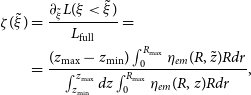 \begin{align}\zeta ({\tilde{\xi}}) & = \frac{\partial_{\tilde{\xi}}L(\xi\lt\tilde{\xi})}{L_{\text{full}}} =\nonumber\\& = \frac{(z_{\max}-z_{\min})\int_{0}^{R_{\max}}\eta_{em}(R,\tilde{z})Rdr}{\int_{z_{\min}}^{z_{\max}}dz \int_{0}^{R_{\max}}\eta_{em}(R,z)Rdr}, \end{align}
where
 $\tilde{\xi}=\xi(\tilde{z})$
,
$\tilde{\xi}=\xi(\tilde{z})$
,
 $z_{NS} (=0)$
– pulsar location.
$z_{NS} (=0)$
– pulsar location.
 $\zeta ({\tilde{\xi}})$
shows to what part of full luminosity in line the unit coordinate
$\zeta ({\tilde{\xi}})$
shows to what part of full luminosity in line the unit coordinate
 $\tilde{\xi}$
corresponds. For uniform distribution of luminosity along a nebula’s tail, the equation holds:
$\tilde{\xi}$
corresponds. For uniform distribution of luminosity along a nebula’s tail, the equation holds:
 $\zeta ({\tilde{\xi}}) = 1$
.
$\zeta ({\tilde{\xi}}) = 1$
.
The profiles for
 $\text{H}_\alpha$
are the closest to uniform luminosity distribution. In the same time, profiles of lines of triply ionized atoms ([C iv], [Ne iv]; see Figure 11) show a spatial lag in growth comparing to others for high pulsar velocities. In v1g53 model, most of the considered lines reach a level of
$\text{H}_\alpha$
are the closest to uniform luminosity distribution. In the same time, profiles of lines of triply ionized atoms ([C iv], [Ne iv]; see Figure 11) show a spatial lag in growth comparing to others for high pulsar velocities. In v1g53 model, most of the considered lines reach a level of
 $\zeta = 0.1$
in
$\zeta = 0.1$
in
 $\tilde{\xi} = 0$
, while for [C iv]
$\tilde{\xi} = 0$
, while for [C iv]
 $\lambda\lambda$
5 803, 5 814 Å doublet and [Ne iv]
$\lambda\lambda$
5 803, 5 814 Å doublet and [Ne iv]
 $\lambda\lambda$
4 714, 4 717, 4 724, 4 726 Å quadruplet that value amounts to
$\lambda\lambda$
4 714, 4 717, 4 724, 4 726 Å quadruplet that value amounts to
 $\tilde{\xi} = 0.1$
. This difference corresponds to 10 a. So ISM starts emitting only in the tail. Such a lag is likely to be caused by the necessity of several ionizations of the atom before emission. In this case, the head of a nebula is expected to have the shape of an open tube.
$\tilde{\xi} = 0.1$
. This difference corresponds to 10 a. So ISM starts emitting only in the tail. Such a lag is likely to be caused by the necessity of several ionizations of the atom before emission. In this case, the head of a nebula is expected to have the shape of an open tube.

Figure 11. Profiles of model nebulae luminosity along tail for models v03g43 and v1g53 (the brightest and the dimmest rings, respectively). Lines are divided into groups by ionization stages and shown on different plots. The luminosity of the nebula in lines is shown next to each of them in brackets.

Figure 12. Model luminosity of the front part of the nebula (
 $z \lt 49.5$
a) averaged over last 100 yr of the simulation versus pulsar velocity. We presented cases of ultrarelativistic gas (
$z \lt 49.5$
a) averaged over last 100 yr of the simulation versus pulsar velocity. We presented cases of ultrarelativistic gas (
 $\gamma = 4/3$
, models v01g43nv, v03g43, v1g43). Lines are divided into groups by ionization stages and shown on different three panels. Error bars show RMS of luminosity.
$\gamma = 4/3$
, models v01g43nv, v03g43, v1g43). Lines are divided into groups by ionization stages and shown on different three panels. Error bars show RMS of luminosity.
There are coinciding peaks in all luminosity profiles, maximum values of which depend on the lines and the models. They correspond to rings in intensity maps. In
 $\text{H}_\alpha$
these peaks are less noticeable, while in [O iii] lines, for example, they are the most luminous parts of the nebula. The brightness of the rings is the lowest in the v1g53 model and the highest in the v03g43 model. Thus, presence of bright and high-contrast rings in the nebula in regions where the density of ISM is highest, may indicate pulsar having an intermediate value of velocity.
$\text{H}_\alpha$
these peaks are less noticeable, while in [O iii] lines, for example, they are the most luminous parts of the nebula. The brightness of the rings is the lowest in the v1g53 model and the highest in the v03g43 model. Thus, presence of bright and high-contrast rings in the nebula in regions where the density of ISM is highest, may indicate pulsar having an intermediate value of velocity.
We expect a disappearance of some elements of the nebula morphology in some cases. In v03g43 and v03g53 models, the first bubble (head of nebula) has little contribution to overall luminosity of the nebula. This effect is stronger for lines of singly ionized atoms than for neutral ones: in v03g43 model
 $\zeta \in [1; 2] \times 10^{-3}$
for [N ii] and [S ii] lines, whereas
$\zeta \in [1; 2] \times 10^{-3}$
for [N ii] and [S ii] lines, whereas
 $\zeta \in [2; 4] \times 10^{-3}$
for [C i] and [N i] lines, and even as high as
$\zeta \in [2; 4] \times 10^{-3}$
for [C i] and [N i] lines, and even as high as
 $3 \times 10^{-2}$
in [O i] lines on the first bubble. The same feature is noticeable for the second bubble – profiles of [N ii] and [S ii] lines lie under
$3 \times 10^{-2}$
in [O i] lines on the first bubble. The same feature is noticeable for the second bubble – profiles of [N ii] and [S ii] lines lie under
 $2 \times 10^{-2}$
and [C i] and [N i] are above, [O i] reaches
$2 \times 10^{-2}$
and [C i] and [N i] are above, [O i] reaches
 $0.1$
. A possible reason is that bubbles, which are in the process of expansion, are smaller than fully developed ones (also a layer between bow shock and contact discontinuity is thinner), and have lower overall luminosity. In v01g43nv model, a similar effect is present – in the same lines, the foremost part of nebula head is dimmer than other regions.
$0.1$
. A possible reason is that bubbles, which are in the process of expansion, are smaller than fully developed ones (also a layer between bow shock and contact discontinuity is thinner), and have lower overall luminosity. In v01g43nv model, a similar effect is present – in the same lines, the foremost part of nebula head is dimmer than other regions.
5.2. Dependence of a nebula luminosity in various lines on pulsar velocity.
We plotted the averaged luminosity of nebulae depending on pulsar velocity (see Figure 12). Because in v01g43nv model morphology developed up to
 $z \approx 50$
a, we limited this analysis to
$z \approx 50$
a, we limited this analysis to
 $z = 49.5$
a. Luminosity was averaged during the last 100 yr of the simulation, error bars correspond to its root mean square (RMS) during a given time. We compared models with different adiabatic index (both
$z = 49.5$
a. Luminosity was averaged during the last 100 yr of the simulation, error bars correspond to its root mean square (RMS) during a given time. We compared models with different adiabatic index (both
 $\gamma = 4/3$
and
$\gamma = 4/3$
and
 $5/3$
) on full length of nebula (
$5/3$
) on full length of nebula (
 $z \le 100$
a) in Appendix B. We show light curves of the model nebulae in Appendix C to illustrate luminosity variability in models. The nebula luminosity strongly depends on pulsar velocity. It can be explained by the ionization stage variation of the element which emits lines. It allows us to understand at which conditions bow-shock PWNe can be bright.
$z \le 100$
a) in Appendix B. We show light curves of the model nebulae in Appendix C to illustrate luminosity variability in models. The nebula luminosity strongly depends on pulsar velocity. It can be explained by the ionization stage variation of the element which emits lines. It allows us to understand at which conditions bow-shock PWNe can be bright.
Most lines of neutral atoms (upper panel of Figure 12) show the strongest monotonic and almost power law dependency. [O i]
 $\lambda\lambda$
6 300, 6 364, 6 394 Å triplet is more than 1.5 order brighter for
$\lambda\lambda$
6 300, 6 364, 6 394 Å triplet is more than 1.5 order brighter for
 $V_{NS}=150$
km/s than for
$V_{NS}=150$
km/s than for
 $1\,500$
km/s. This line is also the brightest multiplet of neutral atoms at
$1\,500$
km/s. This line is also the brightest multiplet of neutral atoms at
 $2 \times 10^{29}$
ergs/s. A second bright multiplet of almost the same luminosity is [N i]
$2 \times 10^{29}$
ergs/s. A second bright multiplet of almost the same luminosity is [N i]
 $\lambda\lambda$
5 198, 5 200 Å, the difference in brightness here is even more and equals 2.5 orders of magnitude. [C i]
$\lambda\lambda$
5 198, 5 200 Å, the difference in brightness here is even more and equals 2.5 orders of magnitude. [C i]
 $\lambda\lambda$
4 622, 4 627 Å doublet is much more faint at
$\lambda\lambda$
4 622, 4 627 Å doublet is much more faint at
 $5 \times 10^{25}$
ergs/s and shows even higher difference in brightness at almost 3 orders of magnitude. We can claim that [O i] and [N i] lines are favourable for observations with luminosity very close to
$5 \times 10^{25}$
ergs/s and shows even higher difference in brightness at almost 3 orders of magnitude. We can claim that [O i] and [N i] lines are favourable for observations with luminosity very close to
 $\text{H}_\alpha$
, but potential target nebulae must contain only low-velocity pulsars (around
$\text{H}_\alpha$
, but potential target nebulae must contain only low-velocity pulsars (around
 $150\,\text{km/s}$
). The exception here is
$150\,\text{km/s}$
). The exception here is
 $\text{H}_\alpha$
line, which luminosity is almost constant and varies in range of
$\text{H}_\alpha$
line, which luminosity is almost constant and varies in range of
 $[4;\,7] \times 10^{29}$
ergs/s. High luminosity in
$[4;\,7] \times 10^{29}$
ergs/s. High luminosity in
 $\text{H}_\alpha$
is natural, because of hydrogen is the most abundant element.
$\text{H}_\alpha$
is natural, because of hydrogen is the most abundant element.
Lines of singly ionized atoms (middle panel on Figure 12) show the same trend, with up to almost 3 orders of magnitude differences in luminosity between velocities. The dependency doesn’t resemble power law like in case of neutral atoms and the ‘knee’ begin to emerge in plots at
 $V_{NS}=450$
km/s. The dependency is monotonic, still with steeper slope at higher pulsar velocity. These lines are favourable for observations with low pulsar velocity also. The brightest sets of lines are [N ii]
$V_{NS}=450$
km/s. The dependency is monotonic, still with steeper slope at higher pulsar velocity. These lines are favourable for observations with low pulsar velocity also. The brightest sets of lines are [N ii]
 $\lambda\lambda$
6 527, 6 548, 6 583 Å triplet and [S ii]
$\lambda\lambda$
6 527, 6 548, 6 583 Å triplet and [S ii]
 $\lambda\lambda$
6 716, 6 731 Å doublet, both peaking at around
$\lambda\lambda$
6 716, 6 731 Å doublet, both peaking at around
 $3 \times 10^{29}$
ergs/s. In the most lines, ‘knee’ is present at almost the same degree, except for faint (
$3 \times 10^{29}$
ergs/s. In the most lines, ‘knee’ is present at almost the same degree, except for faint (
 $L \lt 4 \times 10^{27}$
ergs/s) [C ii] lines. There it transforms to ‘plateau’ with constant luminosity between
$L \lt 4 \times 10^{27}$
ergs/s) [C ii] lines. There it transforms to ‘plateau’ with constant luminosity between
 $V_{NS}=150$
and
$V_{NS}=150$
and
 $450\,\text{km/s}$
. Decrease after
$450\,\text{km/s}$
. Decrease after
 $V_{NS}=450\,\text{km/s}$
is also lower than of other lines.
$V_{NS}=450\,\text{km/s}$
is also lower than of other lines.
Luminosity of doubly and triply ionized atoms lines vs velocity is no longer monotonic with maximum at
 $V_{NS}=450\,\text{km/s}$
. The tendency is following, the higher ionization stage the higher velocity required for the peak. The [O iii]
$V_{NS}=450\,\text{km/s}$
. The tendency is following, the higher ionization stage the higher velocity required for the peak. The [O iii]
 $\lambda\lambda$
4 933, 4 959, 5 007 Å nebular triplet of is brightest and is in perspective for detection. Luminosity in these lines are about
$\lambda\lambda$
4 933, 4 959, 5 007 Å nebular triplet of is brightest and is in perspective for detection. Luminosity in these lines are about
 $2 \times 10^{29}$
ergs/s (peaking at
$2 \times 10^{29}$
ergs/s (peaking at
 $3 \times 10^{29}$
ergs/s) from
$3 \times 10^{29}$
ergs/s) from
 $V_{NS}=150$
km/s till 550 km/s, which makes nearly all known bow-shock PWNe potential candidates for observations. Together with concentration of luminosity in rings, this makes [O iii] lines quite promising.
$V_{NS}=150$
km/s till 550 km/s, which makes nearly all known bow-shock PWNe potential candidates for observations. Together with concentration of luminosity in rings, this makes [O iii] lines quite promising.
6. Discussion and conclusion
In this work, we combine hydrodynamic simulations and non-LTE modelling of line transitions of atomic and ionic species to produce expected intensity maps that allow to reconstruct both density and chemical composition structure in ISM at ultra-small scales.
We developed Shu (Nikonorov Reference Nikonorov2023) program package. It allows calculation of non-LTE intensity maps (analogues of frames in narrowband filters) in more than 150 spectral lines of H, He, C, N, O, S, Ne atoms and their ions for different angles between model axes and picture plane. We used Shu to build synthetic intensity maps of model bow-shock PWNe in various optical lines (listed in Table 4).
A particularly promising application of the present work is to the interaction of the fast-moving pulsar with dilute warm component of ISM, which otherwise is hard to observe. We demonstrate that in this case, one expects relatively bright line emission.
As neutral hydrogen propagates through a nonradiative shock, the
 $\text{H}_\alpha$
emission line exhibits linear polarization. This effect stems from anisotropic excitation by fast-moving electrons and protons, a mechanism supported by observations of SN 1006 (see Sparks et al. Reference Sparks, Pringle, Carswell, Long and Cracraft2015). In the case of PWN, the characteristic shock speed is about 100 km/s, so the polarisation degree should be less than 0.1% (see Laming Reference Laming1990).
$\text{H}_\alpha$
emission line exhibits linear polarization. This effect stems from anisotropic excitation by fast-moving electrons and protons, a mechanism supported by observations of SN 1006 (see Sparks et al. Reference Sparks, Pringle, Carswell, Long and Cracraft2015). In the case of PWN, the characteristic shock speed is about 100 km/s, so the polarisation degree should be less than 0.1% (see Laming Reference Laming1990).
For the majority of observed objects, there are only two significant free parameters: external density structure and angle between pulsar velocity and picture plane. The second one can potentially be found from panoramic spectroscopy (see de Vries et al. Reference de Vries2022) or from direct morphology comparison with models, while the first one is a major question of interest. As we provide the first direct comparison between results of hydrodynamic modelling and observations of Brownsberger & Romani (Reference Brownsberger and Romani2014), the road becomes open to tune the model parameters to reconstruct the structure of ISM inhomogeneities and clouds.
Various lines are formed by ISM inhomogeneities in different locations, showing various morphological features. This fact can be used to reconstruct the abundance structure of different elements. There is also a possibility to obtain the abundance structure of elements using data from different ions (for example, O from [O i] and [O iii], N from [N i] and [N ii]). Realization of this possibility can be done after successful detection of bow-shock PWNe in several lines and can be a unique source of information about warm component of ISM.
We predict the expected features of bow-shock PWNe morphology in various spectral lines and built profiles along the tail for their quantitative description. Peaks in all luminosity profiles correspond to rings on intensity maps. In
 $\text{H}_\alpha$
these peaks are less noticeable, while in [O iii] lines they contain the most part of the nebula luminosity. Profiles of lines of triply ionized atoms ([C iv] and [Ne iv]) show a spatial lag in growth comparing to others for high pulsar velocities. In this case, a head of a nebula is expected to have a shape of an open tube. Seeming disappearance of some elements of nebula morphology due to low intensity relative to other regions is expected in some cases.
$\text{H}_\alpha$
these peaks are less noticeable, while in [O iii] lines they contain the most part of the nebula luminosity. Profiles of lines of triply ionized atoms ([C iv] and [Ne iv]) show a spatial lag in growth comparing to others for high pulsar velocities. In this case, a head of a nebula is expected to have a shape of an open tube. Seeming disappearance of some elements of nebula morphology due to low intensity relative to other regions is expected in some cases.
We predict expected luminosity and favourable conditions for observations in spectral lines of optical range. [O i]
 $\lambda\lambda$
6 300, 6 364, 6 394 Å, [N i]
$\lambda\lambda$
6 300, 6 364, 6 394 Å, [N i]
 $\lambda\lambda$
5 198, 5 200 Å, [N ii]
$\lambda\lambda$
5 198, 5 200 Å, [N ii]
 $\lambda\lambda$
6 527, 6 548, 6 583 Å and [S ii]
$\lambda\lambda$
6 527, 6 548, 6 583 Å and [S ii]
 $\lambda\lambda$
6 716, 6 731 Å are expected to be bright in nebulae of relatively slow pulsars (up to
$\lambda\lambda$
6 716, 6 731 Å are expected to be bright in nebulae of relatively slow pulsars (up to
 $3 \times 10^{29}$
ergs/s for
$3 \times 10^{29}$
ergs/s for
 $V_{NS}=150$
km/s), but aren’t expected to be observable at higher velocities. [O iii]
$V_{NS}=150$
km/s), but aren’t expected to be observable at higher velocities. [O iii]
 $\lambda\lambda$
4 933, 4 959, 5 007 Å lines are expected to be bright (
$\lambda\lambda$
4 933, 4 959, 5 007 Å lines are expected to be bright (
 $[2;\,3]\times 10^{29}$
ergs/s) from
$[2;\,3]\times 10^{29}$
ergs/s) from
 $V_{NS}=150$
km/s to 550 km/s, what makes them the most promising candidate for observations. This makes bow-shock PWNe are potential targets for observations by both earth-based 4m+ telescopes and space telescopes.
$V_{NS}=150$
km/s to 550 km/s, what makes them the most promising candidate for observations. This makes bow-shock PWNe are potential targets for observations by both earth-based 4m+ telescopes and space telescopes.
We calculated five 2D relativistic hydrodynamic models of bow-shock PWNe with detailed accounting for ionization state of H, He, C, N, O, S and Ne. We considered pulsar velocities of
 $V_{NS}=150$
km/s, 450 km/s, and
$V_{NS}=150$
km/s, 450 km/s, and
 $1\,500$
km/s and adiabatic index in ultrarelativistic (
$1\,500$
km/s and adiabatic index in ultrarelativistic (
 $\gamma=4/3$
) and classical (
$\gamma=4/3$
) and classical (
 $\gamma=5/3$
) limit. Periodic variation of interstellar gas density due to inhomogeneities of ISM was included.
$\gamma=5/3$
) limit. Periodic variation of interstellar gas density due to inhomogeneities of ISM was included.
We compared our models to existing observations of bow-shock PWNe. We scaled optical fluxes in
 $\text{H}_\alpha$
(Brownsberger & Romani Reference Brownsberger and Romani2014) with ANTF (Manchester et al. Reference Manchester, Hobbs, Teoh and Hobbs2005) data from radio spectral range. Scaled luminosity in most cases show coincidence with models with accuracy of about 30%. Dependency of nebula luminosity from pulsar velocity obtained from models puts some constraints on flux scaling laws (
$\text{H}_\alpha$
(Brownsberger & Romani Reference Brownsberger and Romani2014) with ANTF (Manchester et al. Reference Manchester, Hobbs, Teoh and Hobbs2005) data from radio spectral range. Scaled luminosity in most cases show coincidence with models with accuracy of about 30%. Dependency of nebula luminosity from pulsar velocity obtained from models puts some constraints on flux scaling laws (
 $\epsilon_{\text{H}\alpha} \eta^2 \propto V_{NS}^{-1}$
). We compared morphology of model nebulae with nebula of PSR J0742-2822. Features of model profiles along nebula tail and observed ones are very similar. Profile of v03g43 model makes the best fit with accuracy of about 30% on most areas.
$\epsilon_{\text{H}\alpha} \eta^2 \propto V_{NS}^{-1}$
). We compared morphology of model nebulae with nebula of PSR J0742-2822. Features of model profiles along nebula tail and observed ones are very similar. Profile of v03g43 model makes the best fit with accuracy of about 30% on most areas.
Despite on overall good agreement of modelled nebulae and observed ones in integrated H
 $_{\alpha}$
flux, there are inconsistencies for several objects, such as J1856-3754, PSR J2225+6535 and in some degree for PSR J0437-4715. However, this fact can be used as a marker of peculiarities of these objects. For example, J1856-3754 is a member of ‘great seven’ and, probably, forms thermal radiation ionization dominated nebulae (Potekhin, De Luca, & Pons Reference Potekhin, De Luca and Pons2015).
$_{\alpha}$
flux, there are inconsistencies for several objects, such as J1856-3754, PSR J2225+6535 and in some degree for PSR J0437-4715. However, this fact can be used as a marker of peculiarities of these objects. For example, J1856-3754 is a member of ‘great seven’ and, probably, forms thermal radiation ionization dominated nebulae (Potekhin, De Luca, & Pons Reference Potekhin, De Luca and Pons2015).
Acknowledgement
The authors appreciated to the anonimous referee for the constructive comments. The simulations were performed on CFCA XC50 cluster of National Astronomical Observatory of Japan (NAOJ) and RIKEN HOKUSAI Bigwaterfall. We thank Alexey Moiseev and Alexander Kolbin for useful discussion and valuable suggestions, Roger Romani for kindly providing the use of observational data of PSR J0742-2822. We acknowledge using python packages numpy (Harris et al. Reference Harris2020), mpi4py (Dalcin & Fang Reference Dalcin and Fang2021), pyCUDA (Klöckner et al. Reference Klöckner, Pinto, Lee, Catanzaro, Ivanov and Fasih2012), astropy (Astropy Collaboration et al. 2022), reproject,Footnote b scipy (Virtanen et al. 2020), matplotlib (Hunter Reference Hunter2007), tueplotsFootnote c and SymPy (Meurer et al. 2017). We used Paraview software (Ayachit,Utkarsh 2015) to plot density maps and streamlines.
Data availability statement
The data underlying this article will be shared on reasonable request to the corresponding author.
Funding statement
This research was supported by the grant 23-22-00385 of the Russian Science Foundation. I.N. Nikonorov acknowledges partial support from Gennady Komissarov Foundation (Appendixes).
Competing interests
None.
Appendix A. Calibration methods
Analytical dependencies of
 $\text{H}_\alpha$
bow-shock PWNe luminosity from various parameters were investigated in Cordes, Romani, & Lundgren (Reference Cordes, Romani and Lundgren1993), Chatterjee & Cordes (Reference Chatterjee and Cordes2002), Brownsberger & Romani (Reference Brownsberger and Romani2014). Various physical assumptions caused complex scaling laws from pulsar velocity. In contrary, we aimed to provide the most general scaling as possible.
$\text{H}_\alpha$
bow-shock PWNe luminosity from various parameters were investigated in Cordes, Romani, & Lundgren (Reference Cordes, Romani and Lundgren1993), Chatterjee & Cordes (Reference Chatterjee and Cordes2002), Brownsberger & Romani (Reference Brownsberger and Romani2014). Various physical assumptions caused complex scaling laws from pulsar velocity. In contrary, we aimed to provide the most general scaling as possible.
Consider an average amount of
 $\text{H}_\alpha$
quanta radiated by one neutral hydrogen atom after passing through a strong shock wave (
$\text{H}_\alpha$
quanta radiated by one neutral hydrogen atom after passing through a strong shock wave (
 $\epsilon_{\text{H}\alpha}$
). Raymond (Reference Raymond1991) estimated the rule of thumb as:
$\epsilon_{\text{H}\alpha}$
). Raymond (Reference Raymond1991) estimated the rule of thumb as:
 \begin{equation} \epsilon_{\text{H}_\alpha} \approx 0.2. \end{equation}
Brownsberger & Romani (Reference Brownsberger and Romani2014) analyse results of numerical simulations of Heng & McCray (Reference Heng and McCray2007), which is estimating radiation of
 $\text{H}_\alpha$
quanta on shock waves. The authors found higher yield for
$\text{H}_\alpha$
quanta on shock waves. The authors found higher yield for
 $V_{NS} \lt 10^3$
km/s in assumption of electron-ion equilibrium behind the shock wave:
$V_{NS} \lt 10^3$
km/s in assumption of electron-ion equilibrium behind the shock wave:
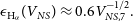 \begin{equation} \epsilon_{\text{H}_\alpha}(V_{NS}) \approx 0.6 V_{NS,7}^{-1/2}. \end{equation}
The authors point out lower yield in non-equilibrium case, which take place at lower pulsar velocities:
 \begin{equation} \epsilon_{\text{H}_\alpha}(V_{NS}) \approx 0.04 V_{NS,7}^{3/4}. \end{equation}
Efficiency in equations (A2) and (A3) equalises on
 $V_{NS} = 8.7 \times 10^2$
km/s and equals to
$V_{NS} = 8.7 \times 10^2$
km/s and equals to
 $\epsilon_{\text{H}_\alpha} = 0.2$
, the estimation of Raymond (Reference Raymond1991). Following equations (A2) and (A3), for models calculated in this work the efficiency should be 0.05, 0.12 and 0.15 for
$\epsilon_{\text{H}_\alpha} = 0.2$
, the estimation of Raymond (Reference Raymond1991). Following equations (A2) and (A3), for models calculated in this work the efficiency should be 0.05, 0.12 and 0.15 for
 $V_{NS}= 150$
, 450 and 1 500 km/s respectively.
$V_{NS}= 150$
, 450 and 1 500 km/s respectively.
We notice that for various conditions behind the shock wave
 $\epsilon_{\text{H}\alpha}$
estimate is either about constant, or some function of ISM material velocity in the shock wave’s frame of reference (which is the same as
$\epsilon_{\text{H}\alpha}$
estimate is either about constant, or some function of ISM material velocity in the shock wave’s frame of reference (which is the same as
 $V_{NS}$
in this work). Serving the purpose of getting the most general law not assuming specific conditions on both sides of the shock wave, we have:
$V_{NS}$
in this work). Serving the purpose of getting the most general law not assuming specific conditions on both sides of the shock wave, we have:
 \begin{equation} \epsilon_{\text{H}_\alpha} = f_1 (V_{NS}), \end{equation}
where
 $f_1 (V_{NS})$
– some function of pulsar velocity.
$f_1 (V_{NS})$
– some function of pulsar velocity.
Barkov, Lyutikov, & Khangulyan (Reference Barkov, Lyutikov and Khangulyan2019) give detailed description of bow-shock PWNe morphology. Consider stand-off distance, which characterise overall size of nebula. The classic equation connecting it with parameters of pulsar and ISM:
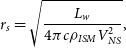 \begin{equation} r_s = \sqrt{\frac{L_w}{4 \pi c \rho_{ISM} V^2_{NS}}}, \end{equation}
where
 $\rho_{ISM}$
– local density of ISM,
$\rho_{ISM}$
– local density of ISM,
 $L_w$
– pulsar luminosity or pulsar spin-down power (
$L_w$
– pulsar luminosity or pulsar spin-down power (
 $\dot{E}$
).
$\dot{E}$
).
Number of hydrogen neutral atoms passing the bow shock during unit time is proportional to ISM density, velocity of pulsar and the area of nebula’s emitting layer (S), which in its turn proportional to stand-off distance squared (
 $r_s^2$
) with some coefficient (
$r_s^2$
) with some coefficient (
 $\eta$
):
$\eta$
):
 \begin{align} L _{\text{H}_\alpha} = \epsilon_{\text{H}\alpha} \rho_{ISM} V_{NS} S\end{align}
 \begin{align}S = \left(\eta r_s\right)^2. \end{align}
In the last case, the proportionality coefficient (
 $\eta$
) depends on the velocity of the pulsar. Cordes, Romani, & Lundgren (Reference Cordes, Romani and Lundgren1993) propose linear dependency:
$\eta$
) depends on the velocity of the pulsar. Cordes, Romani, & Lundgren (Reference Cordes, Romani and Lundgren1993) propose linear dependency:
 \begin{equation} \eta \approx 30 V_{NS, 7}. \end{equation}
Chatterjee & Cordes (Reference Chatterjee and Cordes2002) suggest more general one with power law:
 \begin{equation} \eta \propto V_{NS}^\beta, \end{equation}
where
 $\beta$
is constant, with conclusion
$\beta$
is constant, with conclusion
 $\beta = 1$
is plausible. This and equation (A1) lead to
$\beta = 1$
is plausible. This and equation (A1) lead to
 $L_{\text{H}_\alpha} \propto \dot{E} V_{NS}$
.
$L_{\text{H}_\alpha} \propto \dot{E} V_{NS}$
.
In order to compare these results with modelling, we consider even more general case with coefficient of proportionality
 $\eta$
being an arbitrary function of pulsar velocity:
$\eta$
being an arbitrary function of pulsar velocity:
 \begin{equation} \eta = f_2(V_{NS}). \end{equation}
In total, we have
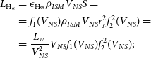 \begin{align}L _{\text{H}_\alpha} &= \epsilon_{\text{H}\alpha} \rho_{ISM} V_{NS} S = \nonumber\\&= f_1(V_{NS}) \rho_{ISM} V_{NS} r_s^2 f_2^2(V_{NS}) =\nonumber\\&=\frac{L_w}{V_{NS}^2} V_{NS} f_1(V_{NS}) f_2^2(V_{NS});\end{align}
 \begin{align}L _{\text{H}_\alpha} = \dot{E} f(V_{NS}),\end{align}
where
 $f(V_{NS}) = V_{NS}^{-1} f_1(V_{NS}) f_2^2(V_{NS})$
– function of
$f(V_{NS}) = V_{NS}^{-1} f_1(V_{NS}) f_2^2(V_{NS})$
– function of
 $V_{NS}$
. It is unknown but is supposed to be common among observed nebulae, disregarding differences in chemical composition and contribution from individual features of morphology.
$V_{NS}$
. It is unknown but is supposed to be common among observed nebulae, disregarding differences in chemical composition and contribution from individual features of morphology.
Thereby, we attained an equation for
 $\text{H}_\alpha$
luminosity calibration to model one for given pulsar velocity:
$\text{H}_\alpha$
luminosity calibration to model one for given pulsar velocity:
 \begin{equation} L_{\text{H}\alpha}^{calibrated} (V_{NS}) = L_{\text{H}\alpha} \dot{E}_{model}(V_{NS}) / \dot{E}. \end{equation}
Here
 $\dot{E}_{model}$
– spin-down power of model pulsar. This quantity corresponds to model
$\dot{E}_{model}$
– spin-down power of model pulsar. This quantity corresponds to model
 $\rho_{ISM} = 1\,m_p/\text{cm}^3$
and
$\rho_{ISM} = 1\,m_p/\text{cm}^3$
and
 $r_s = 0.57$
a, and given
$r_s = 0.57$
a, and given
 $V_{NS}$
, according to equation (A5).
$V_{NS}$
, according to equation (A5).
Appendix B. Luminosity comparison between models
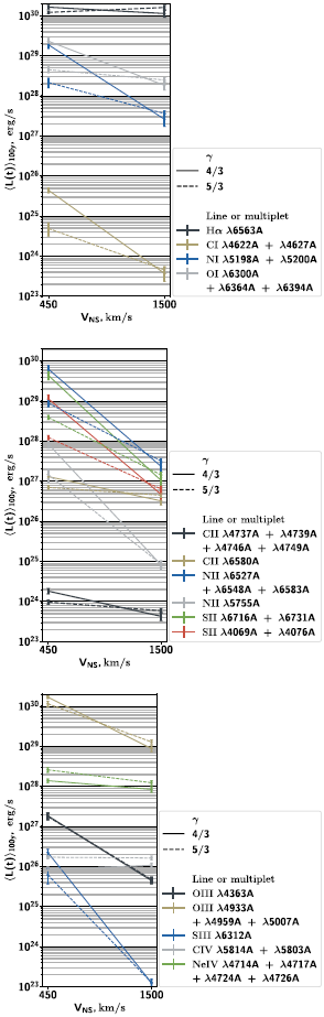
Figure B1. Model luminosity of the nebula (
 $z \lt 100$
a) averaged over last 100 yr of simulation versus pulsar velocity. Here cases of intermediate and high velocities with adiabatic index in both of ultrarelativistic and classical limits are presented (models v03g43, v03g53, v1g43, v1g43). Lines are divided into groups by ionization stages index and presented on different plots. Error bars show standard deviation of luminosity during time of averaging.
$z \lt 100$
a) averaged over last 100 yr of simulation versus pulsar velocity. Here cases of intermediate and high velocities with adiabatic index in both of ultrarelativistic and classical limits are presented (models v03g43, v03g53, v1g43, v1g43). Lines are divided into groups by ionization stages index and presented on different plots. Error bars show standard deviation of luminosity during time of averaging.
On Figure B1 we present a luminosity comparison between models with adiabatic index in ultrarelativistic (
 $\gamma = 4/3$
) and classical (
$\gamma = 4/3$
) and classical (
 $\gamma = 5/3$
) limits on the full length of nebula tail (
$\gamma = 5/3$
) limits on the full length of nebula tail (
 $z \lt 100$
a).
$z \lt 100$
a).
For high pulsar velocity (
 $V_{NS} = 1\,500$
km/s) the difference between luminosity in the same line between models with different adiabatic index is less than variations of luminosity. For intermediate value of velocity (
$V_{NS} = 1\,500$
km/s) the difference between luminosity in the same line between models with different adiabatic index is less than variations of luminosity. For intermediate value of velocity (
 $V_{NS} = 450$
km/s) the situation is the same with
$V_{NS} = 450$
km/s) the situation is the same with
 $\text{H}_\alpha$
and [O iii] lines.
$\text{H}_\alpha$
and [O iii] lines.
The difference is distinctly larger (up to an order of magnitude) in the cases of such bright lines as [N i], [O i], [N ii] and [S ii]. However, this difference is due to the morphology of the nebula. With
 $\gamma = 5/3$
rings are bigger and doesn’t form well in model domain (see Figures 2 and 3). This trait is caused by limitation of numerical scheme and consequently insufficient compression of the relativistic pulsar wind. In real nebulae, we expect rings to form and be visible, even with lower density, than in the case of
$\gamma = 5/3$
rings are bigger and doesn’t form well in model domain (see Figures 2 and 3). This trait is caused by limitation of numerical scheme and consequently insufficient compression of the relativistic pulsar wind. In real nebulae, we expect rings to form and be visible, even with lower density, than in the case of
 $\gamma = 4/3$
.
$\gamma = 4/3$
.

Figure C1. Light curves of nebula in v03g43 and v1g53 (the brightest and the dimmest rings, respectively). Lines are divided into groups by ionization stages and shown on different plots.
Appendix C. Light curves of the model nebulae
Here, we plot light curves of model nebulae following equation:
 \begin{equation} L (t) = \int_{z_{\min}}^{z_{\max}} dz \int_{0}^{R_{\max}} 4 \pi \eta_{em} \left( (R,z), t \right) 2 \pi R dR.\end{equation}
The example light curves are provided in Figure C1.
At the start of the integration, there is no partially ionized gas in the model, so the luminosity in different lines is zero. During the simulation, the quasistationar ionization regime on the bow shock settles, which leads to rapid rise of luminosity until it reaches the plateau. This happens relatively fast in the case of
 $\text{H}_\alpha$
and slower for lines of elements in higher ionization stages.
$\text{H}_\alpha$
and slower for lines of elements in higher ionization stages.
When the quasistationar solution is achieved, there is some variability on light curves. The reason is the difference between the shape of model nebulae and Mach cone. The rise of luminosity is due to rings emerging, enlarging, and thus carrying more material. Then luminosity rapidly falls back to the plateau, when the ring exits computational domain.


 Open access