


1 Introduction
An interesting and important problem in number theory is to understand the size of the class group, known as the class number, for a given field. The case of quadratic extensions of
 $\mathbb{Q}$
has a rich history of investigation that extends back to Gauß. Let
$\mathbb{Q}$
has a rich history of investigation that extends back to Gauß. Let
 $d$
be a fundamental discriminant and
$d$
be a fundamental discriminant and
 $h_{d}$
represent the class number of the field
$h_{d}$
represent the class number of the field
 $\mathbb{Q}(\sqrt{d})$
. Describing the extreme values of
$\mathbb{Q}(\sqrt{d})$
. Describing the extreme values of
 $h_{d}$
and the distribution of these values has been widely investigated. The main line of attack in this problem is to study the moments of
$h_{d}$
and the distribution of these values has been widely investigated. The main line of attack in this problem is to study the moments of
 $L(1,\unicode[STIX]{x1D712}_{d})$
, with
$L(1,\unicode[STIX]{x1D712}_{d})$
, with
 $\unicode[STIX]{x1D712}_{d}$
taken as the Kronecker symbol
$\unicode[STIX]{x1D712}_{d}$
taken as the Kronecker symbol
 $(\frac{d}{\cdot })$
. This approach works because of Dirichlet’s class number formula. Some recent notable papers discussing this problem are those of Granville and Soundararajan [Reference Granville and Soundararajan7] and Dahl and Lamzouri [Reference Dahl and Lamzouri6]. The approach in these articles is to compare the complex moments of
$(\frac{d}{\cdot })$
. This approach works because of Dirichlet’s class number formula. Some recent notable papers discussing this problem are those of Granville and Soundararajan [Reference Granville and Soundararajan7] and Dahl and Lamzouri [Reference Dahl and Lamzouri6]. The approach in these articles is to compare the complex moments of
 $L(1,\unicode[STIX]{x1D712}_{d})$
to that of a random model and use the class number formula to apply this information to
$L(1,\unicode[STIX]{x1D712}_{d})$
to that of a random model and use the class number formula to apply this information to
 $h_{d}$
.
$h_{d}$
.
Here we discuss the adaptation of these techniques to study the class number, denoted as
 $h_{D}$
, over function fields,
$h_{D}$
, over function fields,
 $\mathbb{F}_{q}(T)$
with
$\mathbb{F}_{q}(T)$
with
 $q\equiv 1~(\hspace{0.2em}{\rm mod}\hspace{0.2em}\,4)$
and
$q\equiv 1~(\hspace{0.2em}{\rm mod}\hspace{0.2em}\,4)$
and
 $D$
a monic square-free polynomial in
$D$
a monic square-free polynomial in
 $\mathbb{F}_{q}[T]$
. In this context,
$\mathbb{F}_{q}[T]$
. In this context,
 $h_{D}=|\text{Pic}({\mathcal{O}}_{D})|$
, where
$h_{D}=|\text{Pic}({\mathcal{O}}_{D})|$
, where
 $\text{Pic}({\mathcal{O}}_{D})$
is the Picard group of the ring of integers
$\text{Pic}({\mathcal{O}}_{D})$
is the Picard group of the ring of integers
 ${\mathcal{O}}_{D}\subseteq \mathbb{F}_{q}(T)(\sqrt{D(T)})$
. Since
${\mathcal{O}}_{D}\subseteq \mathbb{F}_{q}(T)(\sqrt{D(T)})$
. Since
 $D$
is a square-free polynomial we have that
$D$
is a square-free polynomial we have that
 $\text{Pic}({\mathcal{O}}_{D})={\mathcal{C}}l({\mathcal{O}}_{D})$
, the class group of
$\text{Pic}({\mathcal{O}}_{D})={\mathcal{C}}l({\mathcal{O}}_{D})$
, the class group of
 ${\mathcal{O}}_{D}$
, which provides the justification for the name “class number”.
${\mathcal{O}}_{D}$
, which provides the justification for the name “class number”.
In 1992, Hoffstein and Rosen [Reference Hoffstein and Rosen9] investigated this question and obtained an average result by fixing the degree of the polynomial. The result is stated as follows: let
 $M$
be odd and positive then
$M$
be odd and positive then
 $$\begin{eqnarray}\frac{1}{q^{M}}\mathop{\sum }_{\substack{ D\text{ monic} \\ \deg (D)=M}}h_{D}=\frac{\unicode[STIX]{x1D701}_{\mathbb{F}_{q}[T]}(2)}{\unicode[STIX]{x1D701}_{\mathbb{F}_{q}[T]}(3)}q^{(M-1)/2}-q^{-1},\end{eqnarray}$$
where
 $$\begin{eqnarray}\unicode[STIX]{x1D701}_{\mathbb{F}_{q}[T]}(s)=\mathop{\sum }_{f\text{ monic}}\frac{1}{|f|^{s}}\quad \text{for }\Re (s)>1,\end{eqnarray}$$
is the Riemann zeta function over
 $\mathbb{F}_{q}[T]$
. Here the norm of
$\mathbb{F}_{q}[T]$
. Here the norm of
 $f\in \mathbb{F}_{q}[T]\setminus \{0\}$
is
$f\in \mathbb{F}_{q}[T]\setminus \{0\}$
is
 $|f|=q^{\deg (f)}$
. This result is directly comparable to Gauß’s conjecture (proven by Siegel [Reference Siegel16]) for class numbers of imaginary quadratic number fields. Finally, letting
$|f|=q^{\deg (f)}$
. This result is directly comparable to Gauß’s conjecture (proven by Siegel [Reference Siegel16]) for class numbers of imaginary quadratic number fields. Finally, letting
 $q\rightarrow \infty$
one obtains an asymptotic formula, which can be compared to the 2012 work of Andrade [Reference Andrade2] described below.
$q\rightarrow \infty$
one obtains an asymptotic formula, which can be compared to the 2012 work of Andrade [Reference Andrade2] described below.
There are two limits that can be considered when studying problems over function fields. The first fixes the degree of the polynomial and lets the number of elements in the base field go to infinity as was done by Hoffstein and Rosen. The second fixes the number of elements in the base field and allows the degree of the polynomials to go to infinity. The result of Andrade [Reference Andrade2] considers the second perspective. His article describes the mean value of
 $h_{D}$
by averaging over
$h_{D}$
by averaging over
 ${\mathcal{H}}_{2g+1}$
the set of monic, square-free polynomials with degree
${\mathcal{H}}_{2g+1}$
the set of monic, square-free polynomials with degree
 $2g+1$
. Proving that
$2g+1$
. Proving that
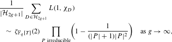
 $$\begin{eqnarray}\displaystyle & & \displaystyle \frac{1}{|{\mathcal{H}}_{2g+1}|}\mathop{\sum }_{D\in {\mathcal{H}}_{2g+1}}h_{D}\nonumber\\ \displaystyle & & \displaystyle \quad \sim \,\unicode[STIX]{x1D701}_{\mathbb{F}_{q}[T]}(2)\mathop{\prod }_{P\text{ irreducible}}\biggl(1-\frac{1}{(|P|+1)|P|^{2}}\biggr)q^{g}\quad \text{as }g\rightarrow \infty .\end{eqnarray}$$
We remark that (1.1) and (1.2) have the same order of magnitude in the main term as can be seen by taking
 $M=2g+1$
.
$M=2g+1$
.
Now, for any monic
 $D\in \mathbb{F}_{q}[T]$
we have Dirichlet characters modulo
$D\in \mathbb{F}_{q}[T]$
we have Dirichlet characters modulo
 $D$
on
$D$
on
 $\mathbb{F}_{q}[T]$
, defined in §2. The natural follow up to this is to define a Dirichlet
$\mathbb{F}_{q}[T]$
, defined in §2. The natural follow up to this is to define a Dirichlet
 $L$
-function associated to such a character:
$L$
-function associated to such a character:
 $$\begin{eqnarray}L(s,\unicode[STIX]{x1D712})=\mathop{\sum }_{f\text{ monic}}\frac{\unicode[STIX]{x1D712}(f)}{|f|^{s}}\quad \text{for }s\in \mathbb{C}.\end{eqnarray}$$
Artin [Reference Artin4] proved a class number formula valid over function fields, which links
 $h_{D}$
to
$h_{D}$
to
 $L(1,\unicode[STIX]{x1D712}_{D})$
, where
$L(1,\unicode[STIX]{x1D712}_{D})$
, where
 $\unicode[STIX]{x1D712}_{D}(\cdot )$
is the Kronecker symbol
$\unicode[STIX]{x1D712}_{D}(\cdot )$
is the Kronecker symbol
 $(\frac{D}{\cdot })$
:
$(\frac{D}{\cdot })$
:
 $$\begin{eqnarray}L(1,\unicode[STIX]{x1D712}_{D})=\frac{\sqrt{q}}{\sqrt{|D|}}h_{D}=q^{-g}h_{D}\quad \text{for }D\in {\mathcal{H}}_{2g+1}.\end{eqnarray}$$
To prove (1.2) Andrade makes use of an approximate functional equation for
 $L(1,\unicode[STIX]{x1D712}_{D})$
to show
$L(1,\unicode[STIX]{x1D712}_{D})$
to show
 $$\begin{eqnarray}\displaystyle & & \displaystyle \frac{1}{|{\mathcal{H}}_{2g+1}|}\mathop{\sum }_{D\in {\mathcal{H}}_{2g+1}}L(1,\unicode[STIX]{x1D712}_{D})\nonumber\\ \displaystyle & & \displaystyle \quad \sim \,\unicode[STIX]{x1D701}_{\mathbb{F}_{q}[T]}(2)\mathop{\prod }_{P\text{ irreducible}}\biggl(1-\frac{1}{(|P|+1)|P|^{2}}\biggr)\quad \text{as }g\rightarrow \infty ,\end{eqnarray}$$
and then applies (1.3). The main drawback to using the approximate functional equation is that it is difficult to use it to calculate large moments of
 $L(1,\unicode[STIX]{x1D712}_{D})$
.
$L(1,\unicode[STIX]{x1D712}_{D})$
.
In this article, we shall investigate the distribution of
 $L(1,\unicode[STIX]{x1D712}_{D})$
for
$L(1,\unicode[STIX]{x1D712}_{D})$
for
 $D\in {\mathcal{H}}_{n}$
as
$D\in {\mathcal{H}}_{n}$
as
 $n\rightarrow \infty$
, where
$n\rightarrow \infty$
, where
 $$\begin{eqnarray}{\mathcal{H}}_{n}=\{D\in \mathbb{F}_{q}[T]:D\text{ is monic, square free, }\deg (D)=n\}.\end{eqnarray}$$
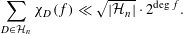
To do this we will need to compute large complex moments of the associated
 $L(1,\unicode[STIX]{x1D712}_{D})$
. We approach the computation of such moments via a random model, a technique that has been used successfully in the study of quadratic number fields.
$L(1,\unicode[STIX]{x1D712}_{D})$
. We approach the computation of such moments via a random model, a technique that has been used successfully in the study of quadratic number fields.
For the remainder of the article the following notation will be fixed. Let
 $\mathbb{A}=\mathbb{F}_{q}[T]$
taking
$\mathbb{A}=\mathbb{F}_{q}[T]$
taking
 $q\equiv 1~(\hspace{0.2em}{\rm mod}\hspace{0.2em}\,4)$
for simplicity. Here
$q\equiv 1~(\hspace{0.2em}{\rm mod}\hspace{0.2em}\,4)$
for simplicity. Here
 $\log$
denotes the base
$\log$
denotes the base
 $q$
logarithm,
$q$
logarithm,
 $\ln$
is the natural logarithm and
$\ln$
is the natural logarithm and
 $\log _{j}$
(respectively
$\log _{j}$
(respectively
 $\ln _{j}$
) represents the
$\ln _{j}$
) represents the
 $j$
-fold iterated logarithm. Finally, let
$j$
-fold iterated logarithm. Finally, let
 $P$
represent an irreducible (prime) polynomial. We define the generalized divisor function
$P$
represent an irreducible (prime) polynomial. We define the generalized divisor function
 $d_{z}(f)$
on its prime powers as
$d_{z}(f)$
on its prime powers as
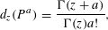 $$\begin{eqnarray}d_{z}(P^{a})=\frac{\unicode[STIX]{x1D6E4}(z+a)}{\unicode[STIX]{x1D6E4}(z)a!},\end{eqnarray}$$
and extend it to all monic polynomials multiplicatively. Then, we can express the complex moments of
 $L(1,\unicode[STIX]{x1D712}_{D})$
as follows.
$L(1,\unicode[STIX]{x1D712}_{D})$
as follows.
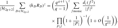
Theorem 1.1. Let
 $n$
a positive integer, and
$n$
a positive integer, and
 $z\in \mathbb{C}$
be such that
$z\in \mathbb{C}$
be such that
 $|z|\leqslant n/(260\log (n)\ln \log (n))$
. Then
$|z|\leqslant n/(260\log (n)\ln \log (n))$
. Then
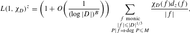
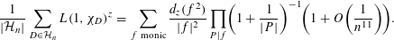 $$\begin{eqnarray}\frac{1}{|{\mathcal{H}}_{n}|}\mathop{\sum }_{D\in {\mathcal{H}}_{n}}L(1,\unicode[STIX]{x1D712}_{D})^{z}=\mathop{\sum }_{\substack{ f~\text{monic}}}\frac{d_{z}(f^{2})}{|f|^{2}}\mathop{\prod }_{P|f}\biggl(1+\frac{1}{|P|}\biggr)^{-1}\biggl(1+O\biggl(\frac{1}{n^{11}}\biggr)\biggr).\end{eqnarray}$$
The strategy for proving this, and a following result about the distribution of values, is to compare the distribution of
 $L(1,\unicode[STIX]{x1D712}_{D})$
to that of a probabilistic random model: let
$L(1,\unicode[STIX]{x1D712}_{D})$
to that of a probabilistic random model: let
 $\{\mathbb{X}(P)\}$
denote a sequence of independent random variables indexed by the irreducible (prime) elements
$\{\mathbb{X}(P)\}$
denote a sequence of independent random variables indexed by the irreducible (prime) elements
 $P\in \mathbb{A}$
, and taking the values
$P\in \mathbb{A}$
, and taking the values
 $0,\pm 1$
as follows:
$0,\pm 1$
as follows:
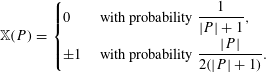 $$\begin{eqnarray}\mathbb{X}(P)=\left\{\begin{array}{@{}ll@{}}\displaystyle 0\quad & \displaystyle \text{ with probability }\frac{1}{|P|+1},\\ \displaystyle \pm 1\quad & \displaystyle \text{ with probability }\frac{|P|}{2(|P|+1)}.\end{array}\right.\end{eqnarray}$$
Let
 $f=P_{1}^{e_{1}}P_{2}^{e_{2}}\cdots P_{s}^{e_{s}}$
be the prime power factorization of
$f=P_{1}^{e_{1}}P_{2}^{e_{2}}\cdots P_{s}^{e_{s}}$
be the prime power factorization of
 $f$
, then we extend the definition of
$f$
, then we extend the definition of
 $\mathbb{X}$
multiplicatively as follows:
$\mathbb{X}$
multiplicatively as follows:
 $$\begin{eqnarray}\mathbb{X}(f)=\mathbb{X}(P_{1})^{e_{1}}\mathbb{X}(P_{2})^{e_{2}}\cdots \mathbb{X}(P_{s})^{e_{s}}.\end{eqnarray}$$
In this article we compare the distribution of
 $L(1,\unicode[STIX]{x1D712}_{D})$
with
$L(1,\unicode[STIX]{x1D712}_{D})$
with
 $$\begin{eqnarray}L(1,\mathbb{X}):=\mathop{\sum }_{f\text{ monic}}\frac{\mathbb{X}(f)}{|f|}=\mathop{\prod }_{P\text{ irreducible}}\biggl(1-\frac{\mathbb{X}(P)}{|P|}\biggr)^{-1},\end{eqnarray}$$
which converges almost surely. Further properties of this model will be discussed in §3.2.
For
 $\unicode[STIX]{x1D70F}>0$
, define
$\unicode[STIX]{x1D70F}>0$
, define
 $$\begin{eqnarray}\unicode[STIX]{x1D6F7}_{\mathbb{X}}(\unicode[STIX]{x1D70F}):=\mathbb{P}(L(1,\mathbb{X})>\text{e}^{\unicode[STIX]{x1D6FE}}\unicode[STIX]{x1D70F})\quad \text{and}\quad \unicode[STIX]{x1D6F9}_{\mathbb{X}}(\unicode[STIX]{x1D70F}):=\mathbb{P}\biggl(L(1,\mathbb{X})<\frac{\unicode[STIX]{x1D701}_{\mathbb{A}}(2)}{\text{e}^{\unicode[STIX]{x1D6FE}}\unicode[STIX]{x1D70F}}\biggr).\end{eqnarray}$$
We prove that the distribution of
 $L(1,\unicode[STIX]{x1D712}_{D})$
is well-approximated by the distribution of
$L(1,\unicode[STIX]{x1D712}_{D})$
is well-approximated by the distribution of
 $L(1,\mathbb{X})$
uniformly in a large range.
$L(1,\mathbb{X})$
uniformly in a large range.
Theorem 1.2. Let
 $n$
be large. Uniformly in
$n$
be large. Uniformly in
 $1\leqslant \unicode[STIX]{x1D70F}\leqslant \log n-2\log _{2}n-\log _{3}n$
we have
$1\leqslant \unicode[STIX]{x1D70F}\leqslant \log n-2\log _{2}n-\log _{3}n$
we have
 $$\begin{eqnarray}\frac{1}{|{\mathcal{H}}_{n}|}|\{D\in {\mathcal{H}}_{n}:L(1,\unicode[STIX]{x1D712}_{D})>\text{e}^{\unicode[STIX]{x1D6FE}}\unicode[STIX]{x1D70F}\}|=\unicode[STIX]{x1D6F7}_{\mathbb{X}}(\unicode[STIX]{x1D70F})\biggl(1+O\biggl(\frac{\text{e}^{\unicode[STIX]{x1D70F}}(\log n)^{2}\log _{2}n}{n}\biggr)\biggr),\end{eqnarray}$$
and
 $$\begin{eqnarray}\frac{1}{|{\mathcal{H}}_{n}|}\biggl|\bigg\{D\in {\mathcal{H}}_{n}:L(1,\unicode[STIX]{x1D712}_{D})<\frac{\unicode[STIX]{x1D701}_{\mathbb{A}}(2)}{\text{e}^{\unicode[STIX]{x1D6FE}}\unicode[STIX]{x1D70F}}\bigg\}\biggr|=\unicode[STIX]{x1D6F9}_{\mathbb{X}}(\unicode[STIX]{x1D70F})\biggl(1+O\biggl(\frac{\text{e}^{\unicode[STIX]{x1D70F}}(\log n)^{2}\log _{2}n}{n}\biggr)\biggr).\end{eqnarray}$$
And below we describe the asymptotic behaviour of
 $\unicode[STIX]{x1D6F7}_{\mathbb{X}}$
and
$\unicode[STIX]{x1D6F7}_{\mathbb{X}}$
and
 $\unicode[STIX]{x1D6F9}_{\mathbb{X}}$
.
$\unicode[STIX]{x1D6F9}_{\mathbb{X}}$
.
Theorem 1.3. For any large
 $\unicode[STIX]{x1D70F}$
we have
$\unicode[STIX]{x1D70F}$
we have
 $$\begin{eqnarray}\unicode[STIX]{x1D6F7}_{\mathbb{X}}(\unicode[STIX]{x1D70F})=\exp \biggl(-C_{1}(q^{\{\log \unicode[STIX]{x1D705}(\unicode[STIX]{x1D70F})\}})\frac{q^{\unicode[STIX]{x1D70F}-C_{0}(q^{\{\log \unicode[STIX]{x1D705}(\unicode[STIX]{x1D70F})\}})}}{\unicode[STIX]{x1D70F}}\biggl(1+O\biggl(\frac{\log \unicode[STIX]{x1D70F}}{\unicode[STIX]{x1D70F}}\biggr)\biggr)\biggr),\end{eqnarray}$$
where
 $\unicode[STIX]{x1D705}(\unicode[STIX]{x1D70F})$
is defined by (4.2),
$\unicode[STIX]{x1D705}(\unicode[STIX]{x1D70F})$
is defined by (4.2),
 $C_{0}(t)=G_{2}(t)$
,
$C_{0}(t)=G_{2}(t)$
,
 $C_{1}(t)=G_{2}(t)-G_{1}(t)$
and
$C_{1}(t)=G_{2}(t)-G_{1}(t)$
and
 $G_{i}(t)$
are defined in (4.7) and (4.9), respectively. Furthermore, we have
$G_{i}(t)$
are defined in (4.7) and (4.9), respectively. Furthermore, we have
 $$\begin{eqnarray}-\frac{1}{\ln q}+\ln (\cosh (c))/c-\tanh (c)<-C_{1}(q^{\{\log \unicode[STIX]{x1D705}(\unicode[STIX]{x1D70F})\}})<\ln (\cosh (q))/q-\tanh (q),\end{eqnarray}$$
where
 $c=1.28377\ldots .$
The same results hold for
$c=1.28377\ldots .$
The same results hold for
 $\unicode[STIX]{x1D713}_{\mathbb{X}}$
.
$\unicode[STIX]{x1D713}_{\mathbb{X}}$
.
Additionally, if we let
 $0<\unicode[STIX]{x1D706}<\text{e}^{-\unicode[STIX]{x1D70F}}$
, then
$0<\unicode[STIX]{x1D706}<\text{e}^{-\unicode[STIX]{x1D70F}}$
, then
 $$\begin{eqnarray}\unicode[STIX]{x1D6F7}_{\mathbb{X}}(\text{e}^{-\unicode[STIX]{x1D706}}\unicode[STIX]{x1D70F})=\unicode[STIX]{x1D6F7}_{\mathbb{ X}}(\unicode[STIX]{x1D70F})(1+O(\unicode[STIX]{x1D706}\text{e}^{\unicode[STIX]{x1D70F}}))\quad \text{and}\quad \unicode[STIX]{x1D6F9}_{\mathbb{ X}}(\text{e}^{-\unicode[STIX]{x1D706}}\unicode[STIX]{x1D70F})=\unicode[STIX]{x1D6F9}_{\mathbb{ X}}(\unicode[STIX]{x1D70F})(1+O(\unicode[STIX]{x1D706}\text{e}^{\unicode[STIX]{x1D70F}})).\end{eqnarray}$$
Our Theorem 1.3 should be compared to those of [Reference Dahl and Lamzouri6, Reference Granville and Soundararajan7], both of which study the behaviour of
 $L(1,\unicode[STIX]{x1D712}_{d})$
over quadratic number fields. The asymptotic behaviour of
$L(1,\unicode[STIX]{x1D712}_{d})$
over quadratic number fields. The asymptotic behaviour of
 $\unicode[STIX]{x1D6F7}_{\mathbb{X}}(\unicode[STIX]{x1D70F})$
is strikingly similar in both of these papers. In [Reference Granville and Soundararajan7] the authors are studying the distribution of
$\unicode[STIX]{x1D6F7}_{\mathbb{X}}(\unicode[STIX]{x1D70F})$
is strikingly similar in both of these papers. In [Reference Granville and Soundararajan7] the authors are studying the distribution of
 $L(1,\unicode[STIX]{x1D712}_{d})$
over all fundamental discriminants
$L(1,\unicode[STIX]{x1D712}_{d})$
over all fundamental discriminants
 $d$
,
$d$
,
 $|d|\leqslant x$
, comparing it to a corresponding probabilistic model
$|d|\leqslant x$
, comparing it to a corresponding probabilistic model
 $L(1,\mathbb{X})$
. In [Reference Dahl and Lamzouri6] the authors are studying the distribution of
$L(1,\mathbb{X})$
. In [Reference Dahl and Lamzouri6] the authors are studying the distribution of
 $L(1,\unicode[STIX]{x1D712}_{d})$
over fundamental discriminants of the form
$L(1,\unicode[STIX]{x1D712}_{d})$
over fundamental discriminants of the form
 $d=4m^{2}+1$
,
$d=4m^{2}+1$
,
 $m\geqslant 1$
and
$m\geqslant 1$
and
 $d$
is square-free. The restriction in [Reference Dahl and Lamzouri6] is used in order to study the behaviour of class numbers associated to such
$d$
is square-free. The restriction in [Reference Dahl and Lamzouri6] is used in order to study the behaviour of class numbers associated to such
 $d$
, again comparing to a corresponding probabilistic model. In both papers
$d$
, again comparing to a corresponding probabilistic model. In both papers
 $\unicode[STIX]{x1D6F7}_{\mathbb{X}}(\unicode[STIX]{x1D70F})=\text{Prob}(L(1,\mathbb{X})>\text{e}^{\unicode[STIX]{x1D6FE}}\unicode[STIX]{x1D70F})$
. Each obtains
$\unicode[STIX]{x1D6F7}_{\mathbb{X}}(\unicode[STIX]{x1D70F})=\text{Prob}(L(1,\mathbb{X})>\text{e}^{\unicode[STIX]{x1D6FE}}\unicode[STIX]{x1D70F})$
. Each obtains
 $$\begin{eqnarray}\unicode[STIX]{x1D6F7}_{\mathbb{X}}(\unicode[STIX]{x1D70F})=\exp \biggl(-C_{1}\frac{\text{e}^{\unicode[STIX]{x1D70F}-C_{0}}}{\unicode[STIX]{x1D70F}}+O\biggl(\frac{\text{e}^{\unicode[STIX]{x1D70F}}}{\unicode[STIX]{x1D70F}^{2}}\biggr)\biggr),\end{eqnarray}$$
where
 $$\begin{eqnarray}C_{1}:=1\quad \text{and}\quad C_{0}:=\int _{0}^{1}\frac{\tanh (t)}{t}\,dt+\int _{1}^{\infty }\frac{\tanh (t)-1}{t}\,dt=0.8187\ldots .\end{eqnarray}$$
Similar behaviour appears when studying the distribution of Euler–Kronecker constants of quadratic fields, see [Reference Lamzouri13, Theorem 1.2] for details. As can be seen from the statement of Theorem 1.3 we observe some pathological behaviour special to function fields. We no longer achieve two constants reflected above as
 $C_{0}$
and
$C_{0}$
and
 $C_{1}$
. In our case the value of both
$C_{1}$
. In our case the value of both
 $C_{0}(q^{\{\log \unicode[STIX]{x1D705}(\unicode[STIX]{x1D70F})\}})$
and
$C_{0}(q^{\{\log \unicode[STIX]{x1D705}(\unicode[STIX]{x1D70F})\}})$
and
 $C_{1}(q^{\{\log \unicode[STIX]{x1D705}(\unicode[STIX]{x1D70F})\}})$
varies, although they remain bounded as the argument varies between
$C_{1}(q^{\{\log \unicode[STIX]{x1D705}(\unicode[STIX]{x1D70F})\}})$
varies, although they remain bounded as the argument varies between
 $1$
and
$1$
and
 $q$
. Figure 1 shows a graph of
$q$
. Figure 1 shows a graph of
 $C_{0}(t)$
for
$C_{0}(t)$
for
 $1\leqslant t<q$
taking
$1\leqslant t<q$
taking
 $q=5$
, and
$q=5$
, and
 $q=9$
the first moduli, which satisfy the hypothesis
$q=9$
the first moduli, which satisfy the hypothesis
 $q\equiv 1~(\hspace{0.2em}{\rm mod}\hspace{0.2em}\,4)$
.
$q\equiv 1~(\hspace{0.2em}{\rm mod}\hspace{0.2em}\,4)$
.
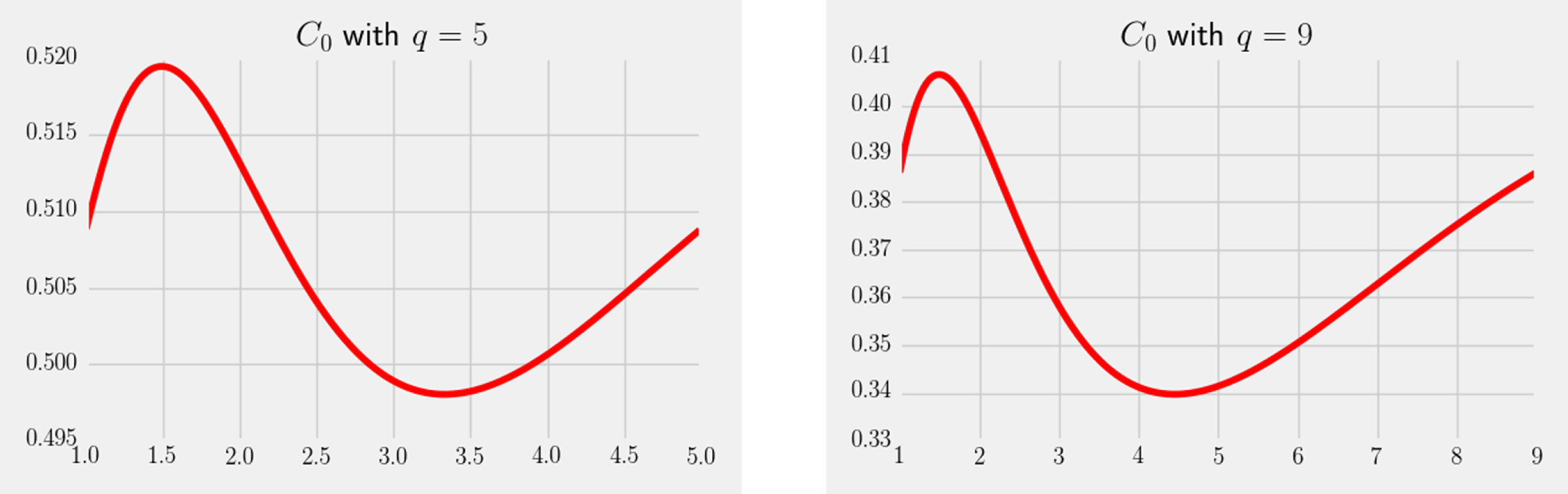
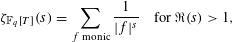
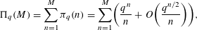
Figure 1 Graph of
 $C_{0}(t)$
, as in Theorem 1.3, for
$C_{0}(t)$
, as in Theorem 1.3, for
 $1\leqslant t\leqslant q$
. The left graph takes
$1\leqslant t\leqslant q$
. The left graph takes
 $q=5$
and the right graph takes
$q=5$
and the right graph takes
 $q=9$
. This is used to describe the range of values that
$q=9$
. This is used to describe the range of values that
 $C_{0}(q^{\{\log \unicode[STIX]{x1D705}(\unicode[STIX]{x1D70F})\}})$
can take and not the graph as
$C_{0}(q^{\{\log \unicode[STIX]{x1D705}(\unicode[STIX]{x1D70F})\}})$
can take and not the graph as
 $\unicode[STIX]{x1D70F}$
changes.
$\unicode[STIX]{x1D70F}$
changes.
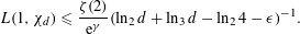
Additionally, we also notice the coefficient
 $C_{1}$
, which appears in all of the theorems describing the behaviour of
$C_{1}$
, which appears in all of the theorems describing the behaviour of
 $\unicode[STIX]{x1D6F7}_{\mathbb{X}}(\unicode[STIX]{x1D70F})$
(cf. [Reference Dahl and Lamzouri6, Reference Granville and Soundararajan7, Reference Lamzouri13]). We find over function fields that the coefficient
$\unicode[STIX]{x1D6F7}_{\mathbb{X}}(\unicode[STIX]{x1D70F})$
(cf. [Reference Dahl and Lamzouri6, Reference Granville and Soundararajan7, Reference Lamzouri13]). We find over function fields that the coefficient
 $C_{1}$
is no longer fixed, but remains bounded between
$C_{1}$
is no longer fixed, but remains bounded between
 $-\text{ln}(\cosh (q))/q+\tanh (q)$
and
$-\text{ln}(\cosh (q))/q+\tanh (q)$
and
 $1/\text{ln}(q)-\ln (\cosh (c))/c+\tanh (c)$
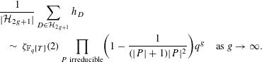
. Figure 2 shows a graph of the behaviour of
$1/\text{ln}(q)-\ln (\cosh (c))/c+\tanh (c)$
. Figure 2 shows a graph of the behaviour of
 $C_{1}(t)$
for
$C_{1}(t)$
for
 $1\leqslant t<q$
with
$1\leqslant t<q$
with
 $q=5$
and
$q=5$
and
 $q=9$
.
$q=9$
.
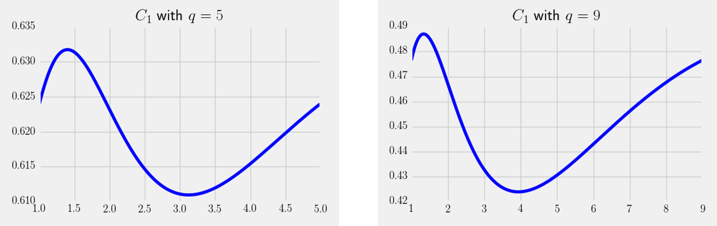
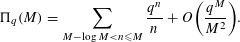
Figure 2 Graph of
 $C_{1}(t)$
, as in Theorem 1.3, for
$C_{1}(t)$
, as in Theorem 1.3, for
 $1\leqslant t\leqslant q$
. The left graph takes
$1\leqslant t\leqslant q$
. The left graph takes
 $q=5$
and the right graph takes
$q=5$
and the right graph takes
 $q=9$
. This is used to describe the range of values that
$q=9$
. This is used to describe the range of values that
 $C_{1}(q^{\{\log \unicode[STIX]{x1D705}(\unicode[STIX]{x1D70F})\}})$
can take and not the graph as
$C_{1}(q^{\{\log \unicode[STIX]{x1D705}(\unicode[STIX]{x1D70F})\}})$
can take and not the graph as
 $\unicode[STIX]{x1D70F}$
changes.
$\unicode[STIX]{x1D70F}$
changes.
The reason for this difference stems from Proposition 4.2, which is used to evaluate the natural log of the real moments of our random model. In this proposition we obtain two sums over primes
 $G_{1}(t)$
and
$G_{1}(t)$
and
 $G_{2}(t)$
, equations (4.7) and (4.9), respectively. The corresponding sums over number fields do not have the parameter
$G_{2}(t)$
, equations (4.7) and (4.9), respectively. The corresponding sums over number fields do not have the parameter
 $t$
(it is always equal to 1), which in our case arises from the way that primes are measured in function fields.
$t$
(it is always equal to 1), which in our case arises from the way that primes are measured in function fields.
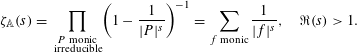
Furthermore, we obtain the following unconditional bounds.
Proposition 1.4. Let
 $F$
be a monic polynomial, and
$F$
be a monic polynomial, and
 $\unicode[STIX]{x1D712}$
be a non-trivial character on
$\unicode[STIX]{x1D712}$
be a non-trivial character on
 $(\mathbb{A}/F\mathbb{A})^{\times }$
. For any complex number
$(\mathbb{A}/F\mathbb{A})^{\times }$
. For any complex number
 $s$
with
$s$
with
 $\text{Re}(s)=1$
we have
$\text{Re}(s)=1$
we have
 $$\begin{eqnarray}\frac{\unicode[STIX]{x1D701}_{\mathbb{A}}(2)}{2\text{e}^{\unicode[STIX]{x1D6FE}}}(\log _{2}|F|+O(1))^{-1}\leqslant |L(s,\unicode[STIX]{x1D712})|\leqslant 2\text{e}^{\unicode[STIX]{x1D6FE}}\log _{2}|F|+O(1).\end{eqnarray}$$
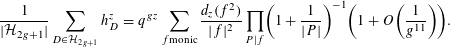
It is important to note that in this setting Weil [Reference Weil17] proved the Riemann hypothesis (RH), and hence these results are achieved unconditionally. We conjecture here that the true size for the extreme values of
 $L(1,\unicode[STIX]{x1D712}_{D})$
is half as large in keeping with the expected results in the quadratic number field case.
$L(1,\unicode[STIX]{x1D712}_{D})$
is half as large in keeping with the expected results in the quadratic number field case.
Conjecture 1.5. Let
 $n$
be large.
$n$
be large.
 $$\begin{eqnarray}\max _{D\in {\mathcal{H}}_{n}}L(1,\unicode[STIX]{x1D712}_{D})=\text{e}^{\unicode[STIX]{x1D6FE}}(\log n+\log _{2}n)+O(1),\end{eqnarray}$$
and
 $$\begin{eqnarray}\min _{D\in {\mathcal{H}}_{n}}L(1,\unicode[STIX]{x1D712}_{D})=\unicode[STIX]{x1D701}_{\mathbb{A}}(2)\text{e}^{-\unicode[STIX]{x1D6FE}}(\log n+\log _{2}n+O(1))^{-1}.\end{eqnarray}$$
Finally, we also unconditionally obtain
 $\unicode[STIX]{x1D6FA}$
-results, which we claim are best possible, unlike in the case of number fields where the corresponding bounds for Dirichlet characters is only valid under the generalized Riemann hypothesis (GRH).
$\unicode[STIX]{x1D6FA}$
-results, which we claim are best possible, unlike in the case of number fields where the corresponding bounds for Dirichlet characters is only valid under the generalized Riemann hypothesis (GRH).
Theorem 1.6. Let
 $N$
be large. There are irreducible polynomials
$N$
be large. There are irreducible polynomials
 $Q_{1}$
and
$Q_{1}$
and
 $Q_{2}$
of degree
$Q_{2}$
of degree
 $N$
such that
$N$
such that
 $$\begin{eqnarray}L(1,\unicode[STIX]{x1D712}_{Q_{1}})\geqslant \text{e}^{\unicode[STIX]{x1D6FE}}(\log _{2}|Q_{1}|+\log _{3}|Q_{1}|)+O(1),\end{eqnarray}$$
and
 $$\begin{eqnarray}L(1,\unicode[STIX]{x1D712}_{Q_{2}})\leqslant \unicode[STIX]{x1D701}_{\mathbb{A}}(2)\text{e}^{-\unicode[STIX]{x1D6FE}}(\log _{2}|Q_{2}|+\log _{3}|Q_{2}|+O(1))^{-1}.\end{eqnarray}$$
The result (1.13) can be compared with [Reference Aisteleitner, Mahatab, Munsch and Peyrot1, Theorem 1] a recent work discussing the size of
 $|L(1,\unicode[STIX]{x1D712})|$
over a number field. The authors prove using a variant of the resonator method that for
$|L(1,\unicode[STIX]{x1D712})|$
over a number field. The authors prove using a variant of the resonator method that for
 $\unicode[STIX]{x1D716}>0$
and sufficiently large
$\unicode[STIX]{x1D716}>0$
and sufficiently large
 $d$
there is a character
$d$
there is a character
 $\unicode[STIX]{x1D712}~(\hspace{0.2em}{\rm mod}\hspace{0.2em}\,d)$
such that
$\unicode[STIX]{x1D712}~(\hspace{0.2em}{\rm mod}\hspace{0.2em}\,d)$
such that
 $$\begin{eqnarray}|L(1,\unicode[STIX]{x1D712})|\geqslant \text{e}^{\unicode[STIX]{x1D6FE}}(\ln _{2}d+\ln _{3}d-(1+\ln _{2}4)-\unicode[STIX]{x1D716}).\end{eqnarray}$$
This result provides an improvement over a paper of Granville and Soundararajan [Reference Granville and Soundararajan8], however, the paper does not give improvements for quadratic characters
 $\unicode[STIX]{x1D712}_{d}$
, where
$\unicode[STIX]{x1D712}_{d}$
, where
 $d$
varies over fundamental discriminants in the range
$d$
varies over fundamental discriminants in the range
 $|d|\leqslant x$
, cf. [Reference Granville and Soundararajan7, Reference Lamzouri12].
$|d|\leqslant x$
, cf. [Reference Granville and Soundararajan7, Reference Lamzouri12].
The result (1.14) can be compared to [Reference Granville and Soundararajan7, Theorem 5a], which under the assumption of GRH proves for any
 $\unicode[STIX]{x1D716}>0$
and all large
$\unicode[STIX]{x1D716}>0$
and all large
 $x$
there are
$x$
there are
 $\gg x^{1/2}$
primes
$\gg x^{1/2}$
primes
 $d\leqslant x$
such that
$d\leqslant x$
such that
 $$\begin{eqnarray}L(1,\unicode[STIX]{x1D712}_{d})\leqslant \frac{\unicode[STIX]{x1D701}(2)}{\text{e}^{\unicode[STIX]{x1D6FE}}}(\ln _{2}d+\ln _{3}d-\ln _{2}4-\unicode[STIX]{x1D716})^{-1}.\end{eqnarray}$$
Unconditionally, for
 $\unicode[STIX]{x1D712}$
a Dirichlet character modulo
$\unicode[STIX]{x1D712}$
a Dirichlet character modulo
 $d$
we have the weaker results
$d$
we have the weaker results
 $|L(1,\unicode[STIX]{x1D712})|\leqslant (\unicode[STIX]{x1D701}(2)/\text{e}^{\unicode[STIX]{x1D6FE}})(\ln _{2}(d)-O(1))^{-1}$
from [Reference Granville and Soundararajan8].
$|L(1,\unicode[STIX]{x1D712})|\leqslant (\unicode[STIX]{x1D701}(2)/\text{e}^{\unicode[STIX]{x1D6FE}})(\ln _{2}(d)-O(1))^{-1}$
from [Reference Granville and Soundararajan8].
1.1 Applications
From the theorems above and in light of (1.3) if we specialize
 $n$
as
$n$
as
 $n=2g+1$
and letting the genus
$n=2g+1$
and letting the genus
 $g\rightarrow \infty$
we can prove analogous results about the class number
$g\rightarrow \infty$
we can prove analogous results about the class number
 $h_{D}$
over
$h_{D}$
over
 ${\mathcal{H}}_{2g+1}$
. This specialization is the equivalent of studying the imaginary quadratic extensions of
${\mathcal{H}}_{2g+1}$
. This specialization is the equivalent of studying the imaginary quadratic extensions of
 $\mathbb{Q}$
, as described by Artin. Below we state a few of the resulting corollaries for
$\mathbb{Q}$
, as described by Artin. Below we state a few of the resulting corollaries for
 $h_{D}$
with
$h_{D}$
with
 $D\in {\mathcal{H}}_{2g+1}$
.
$D\in {\mathcal{H}}_{2g+1}$
.
Corollary 1.7. Let
 $z\in \mathbb{C}$
be such that
$z\in \mathbb{C}$
be such that
 $|z|\leqslant g/(130\log (g)\ln \log (g))$
. Then
$|z|\leqslant g/(130\log (g)\ln \log (g))$
. Then
 $$\begin{eqnarray}\frac{1}{|{\mathcal{H}}_{2g+1}|}\mathop{\sum }_{D\in {\mathcal{H}}_{2g+1}}h_{D}^{z}=q^{gz}\mathop{\sum }_{\substack{ f\text{monic}}}\frac{d_{z}(f^{2})}{|f|^{2}}\mathop{\prod }_{P|f}\biggl(1+\frac{1}{|P|}\biggr)^{-1}\biggl(1+O\biggl(\frac{1}{g^{11}}\biggr)\biggr).\end{eqnarray}$$
This result follows from applying Artin’s class number formula (1.3) to Theorem 1.1 when
 $n=2g+1$
. Additionally, from Theorems 1.2 and 1.3 we obtain that the tail of the distribution of large (and small) values of
$n=2g+1$
. Additionally, from Theorems 1.2 and 1.3 we obtain that the tail of the distribution of large (and small) values of
 $h_{D}$
over
$h_{D}$
over
 ${\mathcal{H}}_{2g+1}$
is doubly exponentially decreasing.
${\mathcal{H}}_{2g+1}$
is doubly exponentially decreasing.
Corollary 1.8. Let
 $g$
be large and
$g$
be large and
 $1\leqslant \unicode[STIX]{x1D70F}\leqslant \log g-2\log _{2}g-\log _{3}g$
. The number of discriminants
$1\leqslant \unicode[STIX]{x1D70F}\leqslant \log g-2\log _{2}g-\log _{3}g$
. The number of discriminants
 $D\in {\mathcal{H}}_{2g+1}$
such that
$D\in {\mathcal{H}}_{2g+1}$
such that
 $$\begin{eqnarray}h_{D}>\text{e}^{\unicode[STIX]{x1D6FE}}\unicode[STIX]{x1D70F}q^{g}\end{eqnarray}$$
equals
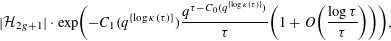 $$\begin{eqnarray}|{\mathcal{H}}_{2g+1}|\cdot \exp \biggl(-C_{1}(q^{\{\log \unicode[STIX]{x1D705}(\unicode[STIX]{x1D70F})\}})\frac{q^{\unicode[STIX]{x1D70F}-C_{0}(q^{\{\log \unicode[STIX]{x1D705}(\unicode[STIX]{x1D70F})\}})}}{\unicode[STIX]{x1D70F}}\biggl(1+O\biggl(\frac{\log \unicode[STIX]{x1D70F}}{\unicode[STIX]{x1D70F}}\biggr)\biggr)\biggr),\end{eqnarray}$$
where
 $\unicode[STIX]{x1D705}(\unicode[STIX]{x1D70F})$
is given by (4.2),
$\unicode[STIX]{x1D705}(\unicode[STIX]{x1D70F})$
is given by (4.2),
 $C_{1}(q^{\{\log \unicode[STIX]{x1D705}(\unicode[STIX]{x1D70F})\}})$
and
$C_{1}(q^{\{\log \unicode[STIX]{x1D705}(\unicode[STIX]{x1D70F})\}})$
and
 $C_{0}(q^{\{\log \unicode[STIX]{x1D705}(\unicode[STIX]{x1D70F})\}})$
are positive constants depending on
$C_{0}(q^{\{\log \unicode[STIX]{x1D705}(\unicode[STIX]{x1D70F})\}})$
are positive constants depending on
 $\unicode[STIX]{x1D70F}$
defined in Theorem 1.3. Similar estimates hold for the number of discriminants
$\unicode[STIX]{x1D70F}$
defined in Theorem 1.3. Similar estimates hold for the number of discriminants
 $D\in {\mathcal{H}}_{2g+1}$
such that
$D\in {\mathcal{H}}_{2g+1}$
such that
 $$\begin{eqnarray}h_{D}<\frac{\unicode[STIX]{x1D701}_{\mathbb{A}}(2)}{\text{e}^{\unicode[STIX]{x1D6FE}}\unicode[STIX]{x1D70F}}q^{g}.\end{eqnarray}$$
Similarly, Proposition 1.4 give analogous upper and lower bounds and Theorem 1.6 provides analogous omega results for
 $h_{D}$
with
$h_{D}$
with
 $D\in {\mathcal{H}}_{2g+1}$
.
$D\in {\mathcal{H}}_{2g+1}$
.
Specializing to
 $n=2g+2$
, we can also make connections to the class number
$n=2g+2$
, we can also make connections to the class number
 $h_{D}$
for
$h_{D}$
for
 $D\in {\mathcal{H}}_{2g+2}$
. This case is analogous to studying a real quadratic extension of
$D\in {\mathcal{H}}_{2g+2}$
. This case is analogous to studying a real quadratic extension of
 $\mathbb{Q}$
and so the class number formula changes. Indeed, for
$\mathbb{Q}$
and so the class number formula changes. Indeed, for
 $D\in {\mathcal{H}}_{2g+2}$
Artin proves
$D\in {\mathcal{H}}_{2g+2}$
Artin proves
 $$\begin{eqnarray}L(1,\unicode[STIX]{x1D712}_{D})=\frac{q-1}{\sqrt{|D|}}h_{D}R_{D},\end{eqnarray}$$
where
 $R_{D}$
denotes the regulator of
$R_{D}$
denotes the regulator of
 ${\mathcal{O}}_{D}$
. In this case
${\mathcal{O}}_{D}$
. In this case
 $R_{D}$
is defined to be
$R_{D}$
is defined to be
 $\log |\unicode[STIX]{x1D716}|_{P_{\infty }}$
, where
$\log |\unicode[STIX]{x1D716}|_{P_{\infty }}$
, where
 $\unicode[STIX]{x1D716}$
is a fundamental unit of
$\unicode[STIX]{x1D716}$
is a fundamental unit of
 ${\mathcal{O}}_{D}$
,
${\mathcal{O}}_{D}$
,
 $P_{\infty }$
is the prime at infinity such that
$P_{\infty }$
is the prime at infinity such that
 $\text{ord}_{P_{\infty }}(\unicode[STIX]{x1D716})<0$
and
$\text{ord}_{P_{\infty }}(\unicode[STIX]{x1D716})<0$
and
 $$\begin{eqnarray}\log |\unicode[STIX]{x1D716}|_{P_{\infty }}=-\text{deg}(P_{\infty })\text{ord}_{P_{\infty }}(\unicode[STIX]{x1D716}).\end{eqnarray}$$
For more details on the regulator see [Reference Rosen15, Ch. 14]. The case of the mean value for
 $L(1,\unicode[STIX]{x1D712}_{D})$
taken over
$L(1,\unicode[STIX]{x1D712}_{D})$
taken over
 ${\mathcal{H}}_{2g+2}$
was investigated by Jung [Reference Jung10, Reference Jung11]. Taking
${\mathcal{H}}_{2g+2}$
was investigated by Jung [Reference Jung10, Reference Jung11]. Taking
 $n=2g+2$
we deduce from (1.15) and Theorem 1.1 the following corollary.
$n=2g+2$
we deduce from (1.15) and Theorem 1.1 the following corollary.
Corollary 1.9. Let
 $z\in \mathbb{C}$
be such that
$z\in \mathbb{C}$
be such that
 $|z|\leqslant g/(130\log (g)\ln \log (g))$
. Then
$|z|\leqslant g/(130\log (g)\ln \log (g))$
. Then
 $$\begin{eqnarray}\displaystyle \frac{1}{|{\mathcal{H}}_{2g+2}|}\mathop{\sum }_{D\in {\mathcal{H}}_{2g+2}}(h_{D}R_{D})^{z} & = & \displaystyle \biggl(\frac{q^{g+1}}{q-1}\biggr)^{z}\mathop{\sum }_{\substack{ f\text{monic}}}\frac{d_{z}(f^{2})}{|f|^{2}}\nonumber\\ \displaystyle & & \displaystyle \times \,\mathop{\prod }_{P|f}\biggl(1+\frac{1}{|P|}\biggr)^{-1}\biggl(1+O\biggl(\frac{1}{g^{11}}\biggr)\biggr).\nonumber\end{eqnarray}$$
Of course, similar results about the distribution of
 $h_{D}R_{D}$
, upper and lower bounds and omega results for
$h_{D}R_{D}$
, upper and lower bounds and omega results for
 $D\in {\mathcal{H}}_{2g+2}$
follow from Theorems 1.2 and 1.3, Proposition 1.4 and Theorem 1.6, respectively.
$D\in {\mathcal{H}}_{2g+2}$
follow from Theorems 1.2 and 1.3, Proposition 1.4 and Theorem 1.6, respectively.
Finally, we give the outline of the paper. Section 2 will establish some facts about
 $\mathbb{A}$
and the properties
$\mathbb{A}$
and the properties
 $L$
-functions have over this ring. Section 3 will connect the complex moments of
$L$
-functions have over this ring. Section 3 will connect the complex moments of
 $L(1,\unicode[STIX]{x1D712}_{D})$
to the expectation of the complex moments of the random model and provide the proof of Theorem 1.7. Section 4 will be used to prove Theorem 1.3. Section 5 proves Theorem 1.2 and Corollary 1.8. Section 6 proves the
$L(1,\unicode[STIX]{x1D712}_{D})$
to the expectation of the complex moments of the random model and provide the proof of Theorem 1.7. Section 4 will be used to prove Theorem 1.3. Section 5 proves Theorem 1.2 and Corollary 1.8. Section 6 proves the
 $\unicode[STIX]{x1D6FA}$
-results of Theorem 1.6.
$\unicode[STIX]{x1D6FA}$
-results of Theorem 1.6.
2 Preliminaries
2.1 Background for function fields
The norm of
 $f\in \mathbb{A}\setminus \{0\}$
is
$f\in \mathbb{A}\setminus \{0\}$
is
 $|f|=q^{\deg (f)}$
and
$|f|=q^{\deg (f)}$
and
 $|0|=0$
. From [Reference Rosen15, Ch. 2] the Riemann zeta function is given by
$|0|=0$
. From [Reference Rosen15, Ch. 2] the Riemann zeta function is given by
 $$\begin{eqnarray}\unicode[STIX]{x1D701}_{\mathbb{A}}(s)=\mathop{\prod }_{\substack{ P\text{ monic} \\ \text{ irreducible}}}\biggl(1-\frac{1}{|P|^{s}}\biggr)^{-1}=\mathop{\sum }_{f\text{ monic}}\frac{1}{|f|^{s}},\quad \Re (s)>1.\end{eqnarray}$$
Since there are
 $q^{k}$
different monic polynomials of degree
$q^{k}$
different monic polynomials of degree
 $k$
, we can also rewrite
$k$
, we can also rewrite
 $\unicode[STIX]{x1D701}_{\mathbb{A}}(s)$
by collecting all the terms with respect to their degree:
$\unicode[STIX]{x1D701}_{\mathbb{A}}(s)$
by collecting all the terms with respect to their degree:
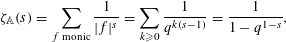 $$\begin{eqnarray}\unicode[STIX]{x1D701}_{\mathbb{A}}(s)=\mathop{\sum }_{f\text{ monic}}\frac{1}{|f|^{s}}=\mathop{\sum }_{k\geqslant 0}\frac{1}{q^{k(s-1)}}=\frac{1}{1-q^{1-s}},\end{eqnarray}$$
which is valid for
 $s\in \mathbb{C}\setminus \{1\}$
. Let
$s\in \mathbb{C}\setminus \{1\}$
. Let
 $$\begin{eqnarray}\unicode[STIX]{x1D70B}_{q}(n)=\#\{a\mid a\text{ monic},\deg (a)=n\text{ and }a\text{ is irreducible}\}.\end{eqnarray}$$
The prime number theorem for polynomials gives the following about
 $\unicode[STIX]{x1D70B}_{q}(n)$
(cf. [Reference Rosen15, Theorem 2.2]):
$\unicode[STIX]{x1D70B}_{q}(n)$
(cf. [Reference Rosen15, Theorem 2.2]):
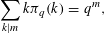 $$\begin{eqnarray}\mathop{\sum }_{k|m}k\unicode[STIX]{x1D70B}_{q}(k)=q^{m},\end{eqnarray}$$
and
 $$\begin{eqnarray}\unicode[STIX]{x1D70B}_{q}(n)=\frac{q^{n}}{n}+O\biggl(\frac{q^{n/2}}{n}\biggr).\end{eqnarray}$$
Let
 $F\in \mathbb{A}$
such that
$F\in \mathbb{A}$
such that
 $\deg (F)>0$
. From [Reference Rosen15, Ch. 4], a Dirichlet character modulo
$\deg (F)>0$
. From [Reference Rosen15, Ch. 4], a Dirichlet character modulo
 $F$
,
$F$
,
 $\unicode[STIX]{x1D712}:\mathbb{A}:\rightarrow \mathbb{C}$
, satisfies:
$\unicode[STIX]{x1D712}:\mathbb{A}:\rightarrow \mathbb{C}$
, satisfies:
(1)
 $\unicode[STIX]{x1D712}(a+bF)=\unicode[STIX]{x1D712}(a)$
for all
$a,b\in \mathbb{A}$
;
$\unicode[STIX]{x1D712}(a+bF)=\unicode[STIX]{x1D712}(a)$
for all
$a,b\in \mathbb{A}$
;(2)
$\unicode[STIX]{x1D712}(a)\unicode[STIX]{x1D712}(b)=\unicode[STIX]{x1D712}(ab)$
for all
$a,b\in \mathbb{A}$
;(3)
$\unicode[STIX]{x1D712}(a)\neq 0\Leftrightarrow (a,F)=1$
.


Then a Dirichlet
 $L$
-function over
$L$
-function over
 $\mathbb{A}$
is given by
$\mathbb{A}$
is given by
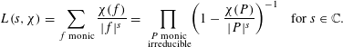 $$\begin{eqnarray}L(s,\unicode[STIX]{x1D712})=\mathop{\sum }_{f\text{ monic}}\frac{\unicode[STIX]{x1D712}(f)}{|f|^{s}}=\mathop{\prod }_{\substack{ P\text{ monic} \\ \text{ irreducible}}}\biggl(1-\frac{\unicode[STIX]{x1D712}(P)}{|P|^{s}}\biggr)^{-1}\quad \text{for }s\in \mathbb{C}.\end{eqnarray}$$
As with
 $\unicode[STIX]{x1D701}_{\mathbb{A}}(s)$
we may collect terms with respect to the degree of the polynomial and write
$\unicode[STIX]{x1D701}_{\mathbb{A}}(s)$
we may collect terms with respect to the degree of the polynomial and write
 $L(s,\unicode[STIX]{x1D712})$
as follows:
$L(s,\unicode[STIX]{x1D712})$
as follows:
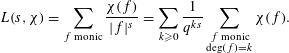 $$\begin{eqnarray}L(s,\unicode[STIX]{x1D712})=\mathop{\sum }_{f\text{ monic}}\frac{\unicode[STIX]{x1D712}(f)}{|f|^{s}}=\mathop{\sum }_{k\geqslant 0}\frac{1}{q^{ks}}\mathop{\sum }_{\substack{ f\text{ monic} \\ \deg (f)=k}}\unicode[STIX]{x1D712}(f).\end{eqnarray}$$
By [Reference Rosen15, Proposition 4.3], if
 $\unicode[STIX]{x1D712}$
is a non-trivial Dirichlet character and
$\unicode[STIX]{x1D712}$
is a non-trivial Dirichlet character and
 $k\geqslant \deg F$
then
$k\geqslant \deg F$
then
 $$\begin{eqnarray}\mathop{\sum }_{\substack{ f\text{ monic} \\ \deg (f)=k}}\unicode[STIX]{x1D712}(f)=0.\end{eqnarray}$$
That is to say that
 $L(s,\unicode[STIX]{x1D712})$
is actually a polynomial in
$L(s,\unicode[STIX]{x1D712})$
is actually a polynomial in
 $q^{-s}$
, whose degree is at most
$q^{-s}$
, whose degree is at most
 $\deg (F)-1$
. Hence, we may also express it as a finite product of linear terms:
$\deg (F)-1$
. Hence, we may also express it as a finite product of linear terms:
 $(1-\unicode[STIX]{x1D6FC}_{j}(\unicode[STIX]{x1D712})q^{-s})$
, for
$(1-\unicode[STIX]{x1D6FC}_{j}(\unicode[STIX]{x1D712})q^{-s})$
, for
 $j=1,2,\ldots ,n\leqslant \deg (F)-1$
.
$j=1,2,\ldots ,n\leqslant \deg (F)-1$
.
Let
 $\unicode[STIX]{x1D6EC}(f)=\deg P$
if
$\unicode[STIX]{x1D6EC}(f)=\deg P$
if
 $f=P^{k}$
and
$f=P^{k}$
and
 $0$
otherwise, the function field analogue of the Von Mangoldt function, then from the proof of [Reference Rosen15, Theorem 4.8] we see
$0$
otherwise, the function field analogue of the Von Mangoldt function, then from the proof of [Reference Rosen15, Theorem 4.8] we see
 $$\begin{eqnarray}\mathop{\sum }_{\substack{ f\text{ monic} \\ \deg (f)=k}}\unicode[STIX]{x1D6EC}(f)\unicode[STIX]{x1D712}(f)=-\mathop{\sum }_{j=1}^{\deg F-1}\unicode[STIX]{x1D6FC}_{j}(\unicode[STIX]{x1D712})^{k}.\end{eqnarray}$$
We mentioned in the introduction that Weil [Reference Weil17] proved the analogue of the RH. In this setting, this says that
 $|\unicode[STIX]{x1D6FC}_{j}(\unicode[STIX]{x1D712})|=1$
or
$|\unicode[STIX]{x1D6FC}_{j}(\unicode[STIX]{x1D712})|=1$
or
 $|\unicode[STIX]{x1D6FC}_{j}(\unicode[STIX]{x1D712})|=\sqrt{q}$
. From this we deduce
$|\unicode[STIX]{x1D6FC}_{j}(\unicode[STIX]{x1D712})|=\sqrt{q}$
. From this we deduce
 $$\begin{eqnarray}\mathop{\sum }_{\deg P=k}\unicode[STIX]{x1D712}(P)\ll \frac{q^{k/2}}{k}\deg F,\end{eqnarray}$$
and that the Euler product representation of
 $L(s,\unicode[STIX]{x1D712})$
 $$\begin{eqnarray}L(s,\unicode[STIX]{x1D712})=\mathop{\prod }_{P}\biggl(1-\frac{\unicode[STIX]{x1D712}(P)}{|P|^{s}}\biggr)^{-1},\end{eqnarray}$$
is actually valid for
 $\text{Re}(s)>1/2$
.
$\text{Re}(s)>1/2$
.
One final remark about the size of
 ${\mathcal{H}}_{n}$
defined in (1.5), if
${\mathcal{H}}_{n}$
defined in (1.5), if
 $n>1$
then from [Reference Rosen15, Proposition 2.3]:
$n>1$
then from [Reference Rosen15, Proposition 2.3]:
 $$\begin{eqnarray}|{\mathcal{H}}_{n}|=q^{n-1}(q-1).\end{eqnarray}$$
Finally, let
 $D\in {\mathcal{H}}_{2g+1}$
. Consider
$D\in {\mathcal{H}}_{2g+1}$
. Consider
 $$\begin{eqnarray}C_{D}:y^{2}=D(x).\end{eqnarray}$$
This defines a hyperelliptic curve over
 $\mathbb{F}_{q}$
with genus
$\mathbb{F}_{q}$
with genus
 $g$
. In this instance
$g$
. In this instance
 $h_{D}$
is associated to the number of
$h_{D}$
is associated to the number of
 $\mathbb{F}_{q}$
-rational points on the Jacobian of
$\mathbb{F}_{q}$
-rational points on the Jacobian of
 $C_{D}$
.
$C_{D}$
.
Let
 $u=q^{-s}$
then the zeta function associated to
$u=q^{-s}$
then the zeta function associated to
 $C_{D}$
is defined by
$C_{D}$
is defined by
 $$\begin{eqnarray}Z_{C_{D}}(s)=\frac{P_{C_{D}}(u)}{(1-u)(1-qu)}.\end{eqnarray}$$
Weil [Reference Weil17] proved
 $P_{C_{D}}(u)$
is a polynomial of degree
$P_{C_{D}}(u)$
is a polynomial of degree
 $2g$
. In fact, from [Reference Rosen15, Propositions 14.6 and 17.7] we have
$2g$
. In fact, from [Reference Rosen15, Propositions 14.6 and 17.7] we have
 $$\begin{eqnarray}P_{C_{D}}(u)=L(s,\unicode[STIX]{x1D712}_{D})=\mathop{\sum }_{f\text{ monic}}\frac{\unicode[STIX]{x1D712}_{D}(f)}{|f|^{s}},\end{eqnarray}$$
where
 $\unicode[STIX]{x1D712}_{D}(f)$
is given by the Kronecker symbol:
$\unicode[STIX]{x1D712}_{D}(f)$
is given by the Kronecker symbol:
 $$\begin{eqnarray}\unicode[STIX]{x1D712}_{D}(f)=\biggl(\frac{D}{f}\biggr)_{2}=\biggl(\frac{D}{f}\biggr).\end{eqnarray}$$
So from the point of view of (1.3) it is natural that
 $h_{D}$
should be associated to this hyperelliptic curve. We note, if
$h_{D}$
should be associated to this hyperelliptic curve. We note, if
 $q\equiv 1\hspace{0.6em}({\rm mod}\hspace{0.2em}4)$
from quadratic reciprocity (cf. [Reference Rosen15, Theorem 3.5]) for any monic polynomials
$q\equiv 1\hspace{0.6em}({\rm mod}\hspace{0.2em}4)$
from quadratic reciprocity (cf. [Reference Rosen15, Theorem 3.5]) for any monic polynomials
 $F,G$
we have
$F,G$
we have
 $$\begin{eqnarray}\biggl(\frac{F}{G}\biggr)=\biggl(\frac{G}{F}\biggr),\end{eqnarray}$$
which explains the assumption we make on
 $q$
.
$q$
.
2.2 Estimates for sums over irreducible monic polynomials
Here and throughout we let
 $\unicode[STIX]{x1D6F1}_{q}(n)$
be the number of monic irreducible polynomials
$\unicode[STIX]{x1D6F1}_{q}(n)$
be the number of monic irreducible polynomials
 $P$
such that
$P$
such that
 $\deg P\leqslant n$
.
$\deg P\leqslant n$
.
Lemma 2.1. Let
 $M$
be a large positive integer. Then we have
$M$
be a large positive integer. Then we have
 $$\begin{eqnarray}\unicode[STIX]{x1D6F1}_{q}(M)=\unicode[STIX]{x1D701}_{\mathbb{A}}(2)\frac{q^{M}}{M}\biggl(1+O\biggl(\frac{\log M}{M}\biggr)\biggr).\end{eqnarray}$$
Proof. Note that
 $$\begin{eqnarray}\unicode[STIX]{x1D6F1}_{q}(M)=\mathop{\sum }_{n=1}^{M}\unicode[STIX]{x1D70B}_{q}(n)=\mathop{\sum }_{n=1}^{M}\biggl(\frac{q^{n}}{n}+O\biggl(\frac{q^{n/2}}{n}\biggr)\biggr),\end{eqnarray}$$
where the last equality comes from the prime number theorem. The main term in this sum is
 $q^{M}/M$
, and we see that if
$q^{M}/M$
, and we see that if
 $n\leqslant M-\log M,$
then
$n\leqslant M-\log M,$
then
 $q^{n}/n\ll q^{M}/M^{2}$
. Hence, we have that
$q^{n}/n\ll q^{M}/M^{2}$
. Hence, we have that
 $$\begin{eqnarray}\unicode[STIX]{x1D6F1}_{q}(M)=\mathop{\sum }_{M-\log M<n\leqslant M}\frac{q^{n}}{n}+O\biggl(\frac{q^{M}}{M^{2}}\biggr).\end{eqnarray}$$
Then for
 $n\in (M-\log M,M]$
we have
$n\in (M-\log M,M]$
we have
 $1/n=(1/M)(1+O(\log M/M)).$
Therefore,
$1/n=(1/M)(1+O(\log M/M)).$
Therefore,
 $$\begin{eqnarray}\displaystyle \unicode[STIX]{x1D6F1}_{q}(M) & = & \displaystyle \frac{q^{M}}{M}\biggl(1+O\biggl(\frac{\log M}{M}\biggr)\biggr)\mathop{\sum }_{l<\log M}\frac{1}{q^{l}}\nonumber\\ \displaystyle & = & \displaystyle \unicode[STIX]{x1D701}_{\mathbb{A}}(2)\frac{q^{M}}{M}\biggl(1+O\biggl(\frac{\log M}{M}\biggr)\biggr).\Box \nonumber\end{eqnarray}$$
Lemma 2.2. Let
 $F$
be a monic polynomial, and
$F$
be a monic polynomial, and
 $\unicode[STIX]{x1D712}$
be a non-trivial character on
$\unicode[STIX]{x1D712}$
be a non-trivial character on
 $(\mathbb{A}/\mathbb{A}F)^{\times }$
. For a positive integer
$(\mathbb{A}/\mathbb{A}F)^{\times }$
. For a positive integer
 $M$
and any complex number
$M$
and any complex number
 $s$
with
$s$
with
 $\text{Re}(s)=1$
we have
$\text{Re}(s)=1$
we have
 $$\begin{eqnarray}\ln L(s,\unicode[STIX]{x1D712})=-\mathop{\sum }_{\deg P\leqslant M}\ln \biggl(1-\frac{\unicode[STIX]{x1D712}(P)}{|P|^{s}}\biggr)+O\biggl(\frac{q^{-M/2}}{M}\deg F\biggr).\end{eqnarray}$$
Proof. Split the sum as
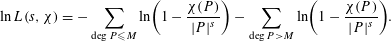 $$\begin{eqnarray}\displaystyle \ln L(s,\unicode[STIX]{x1D712})=-\mathop{\sum }_{\deg P\leqslant M}\ln \biggl(1-\frac{\unicode[STIX]{x1D712}(P)}{|P|^{s}}\biggr)-\mathop{\sum }_{\deg P>M}\ln \biggl(1-\frac{\unicode[STIX]{x1D712}(P)}{|P|^{s}}\biggr). & & \displaystyle \nonumber\end{eqnarray}$$
The error term follows from (2.5) as below
 $$\begin{eqnarray}\displaystyle \mathop{\sum }_{k>M}\mathop{\sum }_{\deg P=k}\ln \biggl(1-\frac{\unicode[STIX]{x1D712}(P)}{|P|}\biggr) & = & \displaystyle \mathop{\sum }_{k>M}\mathop{\sum }_{\deg P=k}\frac{\unicode[STIX]{x1D712}(P)}{|P|^{s}}+O\biggl(\mathop{\sum }_{\deg P>M}\frac{1}{|P|^{2}}\biggr)\nonumber\\ \displaystyle & = & \displaystyle \mathop{\sum }_{k>M}\frac{1}{q^{k}}\mathop{\sum }_{\deg P=k}\unicode[STIX]{x1D712}(P)+O(q^{-M})\nonumber\\ \displaystyle & \ll & \displaystyle \deg F\mathop{\sum }_{k>M}\frac{1}{kq^{k/2}}\nonumber\\ \displaystyle & \ll & \displaystyle \deg F\frac{q^{-M/2}}{M}.\Box \nonumber\end{eqnarray}$$
We now prove a refined form of a Mertens-type estimate due to Rosen [Reference Rosen14].
Lemma 2.3. Let
 $M$
be large. Then, we have
$M$
be large. Then, we have
 $$\begin{eqnarray}-\!\mathop{\sum }_{\deg P\leqslant M}\ln \biggl(1-\frac{1}{|P|}\biggr)=\ln M+\unicode[STIX]{x1D6FE}+\frac{1}{2M}+O\biggl(\frac{1}{M^{2}}\biggr).\end{eqnarray}$$
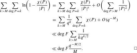
Proof. We have
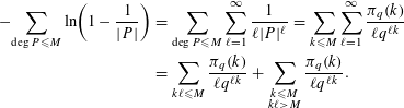 $$\begin{eqnarray}\displaystyle -\!\mathop{\sum }_{\deg P\leqslant M}\ln \biggl(1-\frac{1}{|P|}\biggr) & = & \displaystyle \mathop{\sum }_{\deg P\leqslant M}\mathop{\sum }_{\ell =1}^{\infty }\frac{1}{\ell |P|^{\ell }}=\mathop{\sum }_{k\leqslant M}\mathop{\sum }_{\ell =1}^{\infty }\frac{\unicode[STIX]{x1D70B}_{q}(k)}{\ell q^{\ell k}}\nonumber\\ \displaystyle & = & \displaystyle \mathop{\sum }_{k\ell \leqslant M}\frac{\unicode[STIX]{x1D70B}_{q}(k)}{\ell q^{\ell k}}+\mathop{\sum }_{\substack{ k\leqslant M \\ k\ell >M}}\frac{\unicode[STIX]{x1D70B}_{q}(k)}{\ell q^{\ell k}}.\nonumber\end{eqnarray}$$
By making the change of variables
 $m=k\ell$
and using (2.1), we deduce that the first sum on the right-hand side of the last identity equals
$m=k\ell$
and using (2.1), we deduce that the first sum on the right-hand side of the last identity equals
 $$\begin{eqnarray}\mathop{\sum }_{k\ell \leqslant M}\frac{\unicode[STIX]{x1D70B}_{q}(k)}{\ell q^{\ell k}}=\mathop{\sum }_{m\leqslant M}\frac{1}{q^{m}m}\mathop{\sum }_{k|m}k\unicode[STIX]{x1D70B}_{q}(k)=\mathop{\sum }_{m\leqslant M}\frac{1}{m}=\ln M+\unicode[STIX]{x1D6FE}+\frac{1}{2M}+O\biggl(\frac{1}{M^{2}}\biggr).\end{eqnarray}$$
The result follows upon noting that
 $$\begin{eqnarray}\displaystyle \mathop{\sum }_{\substack{ k\leqslant M \\ k\ell >M}}\frac{\unicode[STIX]{x1D70B}_{q}(k)}{\ell q^{\ell k}} & \ll & \displaystyle \mathop{\sum }_{\substack{ k\leqslant M \\ k\ell >M}}q^{k(1-\ell )}\ll \mathop{\sum }_{2\leqslant \ell \leqslant M}~\mathop{\sum }_{M/\ell <k\leqslant M}q^{k(1-\ell )}+q^{-M}\nonumber\\ \displaystyle & \ll & \displaystyle q^{-M}\mathop{\sum }_{2\leqslant \ell \leqslant M}q^{M/\ell }\ll q^{-M/2}.\Box \nonumber\end{eqnarray}$$
2.3 Proof of Proposition 1.4
Proof of Proposition 1.4.
For
 $\text{Re}(s)=1$
, we use Lemma 2.2 and together with the choice
$\text{Re}(s)=1$
, we use Lemma 2.2 and together with the choice
 $M=2\log \log |F|$
to get
$M=2\log \log |F|$
to get
 $$\begin{eqnarray}\ln L(s,\unicode[STIX]{x1D712})=-\mathop{\sum }_{\deg P\leqslant M}\ln \biggl(1-\frac{\unicode[STIX]{x1D712}(P)}{|P|^{s}}\biggr)+O\biggl(\frac{1}{M}\biggr).\end{eqnarray}$$
Using this estimate together with Lemma 2.3 we deduce that
 $$\begin{eqnarray}|L(s,\unicode[STIX]{x1D712})|\leqslant \mathop{\prod }_{\deg P\leqslant M}\biggl(1-\frac{1}{|P|}\biggr)^{-1}\biggl(1+O\biggl(\frac{1}{M}\biggr)\biggr)\leqslant \text{e}^{\unicode[STIX]{x1D6FE}}M+O(1),\end{eqnarray}$$
which completes the proof of the upper bound in (1.12). To see the lower bound, note that from Lemma 2.2 we have
 $$\begin{eqnarray}|L(s,\unicode[STIX]{x1D712})|\geqslant \mathop{\prod }_{\deg (P)\leqslant M}\biggl(1+\frac{1}{|P|}\biggr)^{-1}\biggl(1+O\biggl(\frac{1}{M}\biggr)\biggr),\end{eqnarray}$$
and from Lemma 2.3
 $$\begin{eqnarray}\mathop{\prod }_{\deg (P)\leqslant M}\biggl(1+\frac{1}{|P|}\biggr)^{-1}=\mathop{\prod }_{\deg (P)\leqslant M}\frac{(1-1/|P|^{2})^{-1}}{(1-1/|P|)^{-1}}\geqslant \frac{\unicode[STIX]{x1D701}_{\mathbb{A}}(2)}{\text{e}^{\unicode[STIX]{x1D6FE}}M+O(1)}.\Box\end{eqnarray}$$
2.4 Sums over
${\mathcal{H}}_{n}$

The orthogonality relation is as follows.
Lemma 2.4. Let
 $f$
be a monic polynomial. If
$f$
be a monic polynomial. If
 $f$
is a square in
$f$
is a square in
 $\mathbb{A}$
, then
$\mathbb{A}$
, then
 $$\begin{eqnarray}\mathop{\sum }_{D\in {\mathcal{H}}_{n}}\unicode[STIX]{x1D712}_{D}(f)=|{\mathcal{H}}_{n}|\cdot \mathop{\prod }_{P\mid f}\biggl(1+\frac{1}{|P|}\biggr)^{-1}+O(\sqrt{|{\mathcal{H}}_{n}|}).\end{eqnarray}$$
Furthermore, if
 $f$
is not a square in
$f$
is not a square in
 $\mathbb{A}$
, then
$\mathbb{A}$
, then
 $$\begin{eqnarray}\mathop{\sum }_{D\in {\mathcal{H}}_{n}}\unicode[STIX]{x1D712}_{D}(f)\ll \sqrt{|{\mathcal{H}}_{n}|}\cdot 2^{\deg f}.\end{eqnarray}$$
Proof. The first estimate follows from [Reference Andrade and Keating3, Proposition 5.2], while the second follows from [Reference Andrade and Keating3, Lemma 6.4]. ◻
Remark 2.5. We remark here that making use of [Reference Bui and Florea5, Lemma 3.5], the second estimate becomes
 $$\begin{eqnarray}\mathop{\sum }_{D\in {\mathcal{H}}_{n}}\unicode[STIX]{x1D712}_{D}(f)\ll \frac{\sqrt{|{\mathcal{H}}_{n}|}}{(q-1)^{1/2}}|f_{1}|^{\unicode[STIX]{x1D716}},\end{eqnarray}$$
for
 $\unicode[STIX]{x1D716}>0$
and
$\unicode[STIX]{x1D716}>0$
and
 $f=f_{1}f_{2}^{2}$
with
$f=f_{1}f_{2}^{2}$
with
 $f_{1}$
square-free. This in turn leads to a better error for the sum over the non-square terms, which is done in Lemma 3.3.
$f_{1}$
square-free. This in turn leads to a better error for the sum over the non-square terms, which is done in Lemma 3.3.
3 Complex moments of
$L(1,\unicode[STIX]{x1D712})$

Let
 $D\in {\mathcal{H}}_{n}$
,
$D\in {\mathcal{H}}_{n}$
,
 $z\in \mathbb{C}$
such that
$z\in \mathbb{C}$
such that
 $|z|\ll \log |D|/(\log _{2}|D|\ln \log _{2}|D|)$
. Let
$|z|\ll \log |D|/(\log _{2}|D|\ln \log _{2}|D|)$
. Let
 $\unicode[STIX]{x1D712}_{D}(f)=(D/f)$
. We recall that
$\unicode[STIX]{x1D712}_{D}(f)=(D/f)$
. We recall that
 $d_{z}(f)$
is defined as in (1.6). We will prove the following key lemma, which will allow us to connect our complex moments of the random model to the complex moments of
$d_{z}(f)$
is defined as in (1.6). We will prove the following key lemma, which will allow us to connect our complex moments of the random model to the complex moments of
 $L(1,\unicode[STIX]{x1D712}_{D})$
.
$L(1,\unicode[STIX]{x1D712}_{D})$
.
Lemma 3.1. Let
 $D\in {\mathcal{H}}_{n}$
. Let
$D\in {\mathcal{H}}_{n}$
. Let
 $A>4$
be a constant
$A>4$
be a constant
 $z\in \mathbb{C}$
such that
$z\in \mathbb{C}$
such that
 $|z|\leqslant \log |D|/(10A\log _{2}|D|\ln \log _{2}|D|)$
and
$|z|\leqslant \log |D|/(10A\log _{2}|D|\ln \log _{2}|D|)$
and
 $M=A\log _{2}|D|$
. Then
$M=A\log _{2}|D|$
. Then
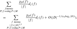
 $$\begin{eqnarray}L(1,\unicode[STIX]{x1D712}_{D})^{z}=\biggl(1+O\biggl(\frac{1}{(\log |D|)^{B}}\biggr)\biggr)\mathop{\sum }_{\substack{ f~\text{monic} \\ |f|\leqslant |D|^{1/3} \\ P|f\Rightarrow \deg P\leqslant M}}\frac{\unicode[STIX]{x1D712}_{D}(f)d_{z}(f)}{|f|},\end{eqnarray}$$
where
 $B=A/2-2$
.
$B=A/2-2$
.
Before giving the proof, we make some estimates.
Lemma 3.2. Let
 $D\in {\mathcal{H}}_{n}$
,
$D\in {\mathcal{H}}_{n}$
,
 $A>4$
be a fixed constant and
$A>4$
be a fixed constant and
 $z\in \mathbb{C}$
such that
$z\in \mathbb{C}$
such that
 $|z|\leqslant \log |D|/(10A\log _{2}|D|\ln \log _{2}|D|)$
and
$|z|\leqslant \log |D|/(10A\log _{2}|D|\ln \log _{2}|D|)$
and
 $M=A\log _{2}|D|$
. Then for
$M=A\log _{2}|D|$
. Then for
 $c_{0}$
some positive constant we have
$c_{0}$
some positive constant we have
 $$\begin{eqnarray}\displaystyle & & \displaystyle \mathop{\sum }_{\substack{ f\text{monic} \\ P|f\Rightarrow \deg P\leqslant M}}\frac{\unicode[STIX]{x1D712}_{D}(f)}{|f|}d_{z}(f)\nonumber\\ \displaystyle & & \displaystyle \quad =\mathop{\sum }_{\substack{ f~\text{monic} \\ |f|\leqslant |D|^{1/3} \\ P|f\Rightarrow \deg P\leqslant M}}\frac{\unicode[STIX]{x1D712}_{D}(f)}{|f|}d_{z}(f)+O(|D|^{-1/(c_{0}\log _{2}|D|)}),\end{eqnarray}$$
and furthermore,
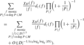 $$\begin{eqnarray}\displaystyle & & \displaystyle \mathop{\sum }_{\substack{ f~\text{monic} \\ P|f\Rightarrow \deg P\leqslant M}}\frac{\unicode[STIX]{x1D712}_{D}(f)}{|f|}d_{z}(f)\mathop{\prod }_{P|f}\biggl(1+\frac{1}{|P|}\biggr)^{-1}\nonumber\\ \displaystyle & & \displaystyle \quad =\mathop{\sum }_{\substack{ f~\text{monic} \\ |f|\leqslant |D|^{1/3} \\ P|f\Rightarrow \deg P\leqslant M}}\frac{\unicode[STIX]{x1D712}_{D}(f)}{|f|}d_{z}(f)\mathop{\prod }_{P|f}\biggl(1+\frac{1}{|P|}\biggr)^{-1}\nonumber\\ \displaystyle & & \displaystyle \qquad +\,O(|D|^{-1/(c_{0}\log _{q}\log _{q}|D|)}).\end{eqnarray}$$
Proof. First we prove (3.1). Let
 $z\in \mathbb{C}$
and let
$z\in \mathbb{C}$
and let
 $k\in \mathbb{Z}$
such that
$k\in \mathbb{Z}$
such that
 $|z|<k$
. Let
$|z|<k$
. Let
 $0<\unicode[STIX]{x1D6FC}\leqslant \frac{1}{2}$
, then using Rankin’s trick we see
$0<\unicode[STIX]{x1D6FC}\leqslant \frac{1}{2}$
, then using Rankin’s trick we see
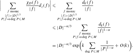 $$\begin{eqnarray}\displaystyle \biggl|\mathop{\sum }_{\substack{ f\text{ monic} \\ |f|>|D|^{1/3} \\ P|f\Rightarrow \deg P\leqslant M}}\frac{\unicode[STIX]{x1D712}_{D}(f)}{|f|}d_{z}(f)\biggr| & {\leqslant} & \displaystyle \mathop{\sum }_{\substack{ f\text{ monic} \\ |f|>|D|^{1/3} \\ P|f\Rightarrow \deg P\leqslant M}}\frac{d_{k}(f)}{|f|}\nonumber\\ \displaystyle & {\leqslant} & \displaystyle |D|^{-\unicode[STIX]{x1D6FC}/3}\mathop{\sum }_{\substack{ f\text{ monic} \\ P|f\Rightarrow \deg P\leqslant M}}\frac{d_{k}(f)}{|f|^{1-\unicode[STIX]{x1D6FC}}}\nonumber\\ \displaystyle & = & \displaystyle |D|^{-\unicode[STIX]{x1D6FC}/3}\exp \biggl(k\mathop{\sum }_{\deg P\leqslant M}\frac{1}{|P|^{1-\unicode[STIX]{x1D6FC}}}+O(k)\biggr).\nonumber\end{eqnarray}$$
Choosing
 $\unicode[STIX]{x1D6FC}=1/M$
we have that
$\unicode[STIX]{x1D6FC}=1/M$
we have that
 $|P|^{\unicode[STIX]{x1D6FC}}=q^{\unicode[STIX]{x1D6FC}\deg P}\leqslant q=O(1)$
, so that
$|P|^{\unicode[STIX]{x1D6FC}}=q^{\unicode[STIX]{x1D6FC}\deg P}\leqslant q=O(1)$
, so that
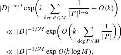 $$\begin{eqnarray}\displaystyle & & \displaystyle |D|^{-\unicode[STIX]{x1D6FC}/3}\exp \biggl(k\mathop{\sum }_{\deg P\leqslant M}\frac{1}{|P|^{1-\unicode[STIX]{x1D6FC}}}+O(k)\biggr)\nonumber\\ \displaystyle & & \displaystyle \quad \ll \,|D|^{-1/3M}\exp \biggl(O\biggl(k\mathop{\sum }_{\deg P\leqslant M}\frac{1}{|P|}\biggr)\biggr)\nonumber\\ \displaystyle & & \displaystyle \quad \ll \,|D|^{-1/3M}\exp O(k\log M),\nonumber\end{eqnarray}$$
by Mertens’ theorem. Taking
 $k\ll \log |D|/(\log _{2}|D|\ln \log _{2}|D|)$
, and using
$k\ll \log |D|/(\log _{2}|D|\ln \log _{2}|D|)$
, and using
 $M=A\log _{2}|D|$
the expression inside of the big
$M=A\log _{2}|D|$
the expression inside of the big
 $O$
becomes
$O$
becomes
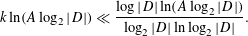 $$\begin{eqnarray}k\ln (A\log _{2}|D|)\ll \frac{\log |D|\ln (A\log _{2}|D|)}{\log _{2}|D|\ln \log _{2}|D|}.\end{eqnarray}$$
So we have
 $$\begin{eqnarray}|D|^{-1/3M}\exp O(k\log M)\ll |D|^{-1/(c_{0}\log _{2}|D|)},\end{eqnarray}$$
for some
 $c_{0}>0$
.
$c_{0}>0$
.
The proof of (3.2) follows from the previous argument since
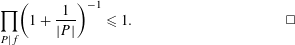 $$\begin{eqnarray}\mathop{\prod }_{P|f}\biggl(1+\frac{1}{|P|}\biggr)^{-1}\leqslant 1.\Box\end{eqnarray}$$
Proof of Lemma 3.1.
From Lemma 2.2 we have
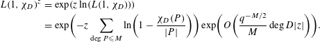 $$\begin{eqnarray}\displaystyle L(1,\unicode[STIX]{x1D712}_{D})^{z} & = & \displaystyle \exp (z\ln (L(1,\unicode[STIX]{x1D712}_{D})))\nonumber\\ \displaystyle & = & \displaystyle \exp \biggl(-z\mathop{\sum }_{\deg P\leqslant M}\ln \biggl(1-\frac{\unicode[STIX]{x1D712}_{D}(P)}{|P|}\biggr)\biggr)\exp \biggl(O\biggl(\frac{q^{-M/2}}{M}\deg D|z|\biggr)\biggr).\nonumber\end{eqnarray}$$
Here we use the fact that
 $M=A\log _{2}|D|$
implying that
$M=A\log _{2}|D|$
implying that
 $q^{-M/2}=(\log |D|)^{-A/2}$
,
$q^{-M/2}=(\log |D|)^{-A/2}$
,
 $\deg D=\log |D|$
,
$\deg D=\log |D|$
,
 $|z|\leqslant \log |D|/(10A\log _{2}|D|\ln \log _{2}|D|)$
to see that the expression inside of the big
$|z|\leqslant \log |D|/(10A\log _{2}|D|\ln \log _{2}|D|)$
to see that the expression inside of the big
 $O$
has the shape
$O$
has the shape
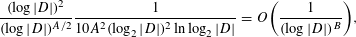 $$\begin{eqnarray}\frac{(\log |D|)^{2}}{(\log |D|)^{A/2}}\frac{1}{10A^{2}(\log _{2}|D|)^{2}\ln \log _{2}|D|}=O\biggl(\frac{1}{(\log |D|)^{B}}\biggr),\end{eqnarray}$$
by the assumption on
 $A$
. Hence, we have
$A$
. Hence, we have
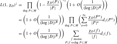 $$\begin{eqnarray}\displaystyle L(1,\unicode[STIX]{x1D712}_{D})^{z} & = & \displaystyle \mathop{\prod }_{\deg P\leqslant M}\biggl(1-\frac{\unicode[STIX]{x1D712}_{D}(P)}{|P|}\biggr)^{-z}\biggl(1+O\biggl(\frac{1}{(\log |D|)^{B}}\biggr)\biggr)\nonumber\\ \displaystyle & = & \displaystyle \biggl(1+O\biggl(\frac{1}{(\log |D|)^{B}}\biggr)\biggr)\mathop{\prod }_{\deg P\leqslant M}\biggl(\mathop{\sum }_{a=0}^{\infty }\frac{\unicode[STIX]{x1D712}_{D}(P^{a})}{|P|^{a}}d_{z}(P^{a})\biggr)\nonumber\\ \displaystyle & = & \displaystyle \biggl(1+O\biggl(\frac{1}{(\log |D|)^{B}}\biggr)\biggr)\mathop{\sum }_{\substack{ f\text{ monic} \\ P|f\Rightarrow \deg P\leqslant M}}\frac{\unicode[STIX]{x1D712}_{D}(f)}{|f|}d_{z}(f).\nonumber\end{eqnarray}$$
Finally, we apply (3.1) from Lemma 3.2, then the relative sizes of the
 $O$
terms completes the result for this case.◻
$O$
terms completes the result for this case.◻
Using this lemma we have that
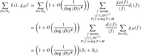 $$\begin{eqnarray}\displaystyle \mathop{\sum }_{D\in {\mathcal{H}}_{n}}L(1,\unicode[STIX]{x1D712}_{D})^{z} & = & \displaystyle \mathop{\sum }_{D\in {\mathcal{H}}_{n}}\biggl(1+O\biggl(\frac{1}{(\log |D|)^{B}}\biggr)\biggr)\mathop{\sum }_{\substack{ f\text{ monic} \\ |f|\leqslant |D|^{1/3} \\ P|f\Rightarrow \deg P\leqslant M}}\frac{\unicode[STIX]{x1D712}_{D}(f)}{|f|}d_{z}(f)\nonumber\\ \displaystyle & = & \displaystyle \biggl(1+O\biggl(\frac{1}{(\log |D|)^{B}}\biggr)\biggr)\mathop{\sum }_{\substack{ f\text{ monic} \\ |f|\leqslant |D|^{1/3} \\ P|f\Rightarrow \deg P\leqslant M}}\frac{d_{z}(f)}{|f|}\mathop{\sum }_{D\in {\mathcal{H}}_{n}}\unicode[STIX]{x1D712}_{D}(f)\nonumber\\ \displaystyle & = & \displaystyle \biggl(1+O\biggl(\frac{1}{(\log |D|)^{B}}\biggr)\biggr)(S_{1}+S_{2}),\nonumber\end{eqnarray}$$
where
 $$\begin{eqnarray}S_{1}:=\mathop{\sum }_{\substack{ f\text{ monic and a square} \\ |f|\leqslant |D|^{1/3} \\ P|f\Rightarrow \deg P\leqslant M}}\frac{d_{z}(f)}{|f|}\mathop{\sum }_{D\in {\mathcal{H}}_{n}}\unicode[STIX]{x1D712}_{D}(f),\end{eqnarray}$$
and
 $$\begin{eqnarray}S_{2}:=\mathop{\sum }_{\substack{ f\text{ monic and not a square} \\ |f|\leqslant |D|^{1/3} \\ P|f\Rightarrow \deg P\leqslant M}}\frac{d_{z}(f)}{|f|}\mathop{\sum }_{D\in {\mathcal{H}}_{n}}\unicode[STIX]{x1D712}_{D}(f).\end{eqnarray}$$
With this separation we can use our orthogonality relation to evaluate
 $S_{1}$
and
$S_{1}$
and
 $S_{2}$
.
$S_{2}$
.
3.1 Evaluating
$S_{2}$
: contribution of the non-square terms

Lemma 3.3. Let
 $D\in {\mathcal{H}}_{n}$
,
$D\in {\mathcal{H}}_{n}$
,
 $A>4$
be a constant,
$A>4$
be a constant,
 $z\in \mathbb{C}$
be such that
$z\in \mathbb{C}$
be such that
 $|z|\leqslant \log |D|/(10A\log _{2}|D|\ln \log _{2}|D|)$
and
$|z|\leqslant \log |D|/(10A\log _{2}|D|\ln \log _{2}|D|)$
and
 $M=A\log _{2}|D|$
. Then
$M=A\log _{2}|D|$
. Then
 $$\begin{eqnarray}\biggl(1+\frac{1}{(\log |D|)^{B}}\biggr)S_{2}\ll |D|^{6/7},\end{eqnarray}$$
with
 $S_{2}$
defined as in (3.4).
$S_{2}$
defined as in (3.4).
Remark 3.4. Making use of Remark 2.5 and following the argument from [Reference Bui and Florea5, p. 12] we can improve this bound to
 $$\begin{eqnarray}\biggl(1+O\biggl(\frac{1}{(\log |D|)^{B}}\biggr)\biggr)S_{2}\ll |D|^{1/2+\unicode[STIX]{x1D716}}.\end{eqnarray}$$
Proof. By Lemma 2.4 the inner sum of
 $S_{2}$
is
$S_{2}$
is
 $O(\sqrt{|{\mathcal{H}}_{n}|}2^{\deg f})$
, and hence we have
$O(\sqrt{|{\mathcal{H}}_{n}|}2^{\deg f})$
, and hence we have
 $$\begin{eqnarray}S_{2}\ll \sqrt{|{\mathcal{H}}_{n}|}\mathop{\sum }_{\substack{ f\text{ monic and not a square} \\ |f|\leqslant |D|^{1/3} \\ P|f\Rightarrow \deg P\leqslant M}}\frac{d_{z}(f)2^{\deg f}}{|f|}.\end{eqnarray}$$
Now, we have that
 $|{\mathcal{H}}_{n}|=O(|D|)$
and
$|{\mathcal{H}}_{n}|=O(|D|)$
and
 $2^{\deg f}=|f|^{\ln 2/\text{ln}\,q}<|f|^{11/25}$
, the last inequality following from the fact that
$2^{\deg f}=|f|^{\ln 2/\text{ln}\,q}<|f|^{11/25}$
, the last inequality following from the fact that
 $q\geqslant 5$
and
$q\geqslant 5$
and
 $\ln 2/\text{ln}\,5=0.43067\ldots .$
Thus,
$\ln 2/\text{ln}\,5=0.43067\ldots .$
Thus,
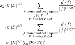 $$\begin{eqnarray}\displaystyle S_{2} & \ll & \displaystyle |D|^{1/2}\mathop{\sum }_{\substack{ f\text{ monic and not a square} \\ |f|\leqslant |D|^{1/3} \\ P|f\Rightarrow \deg P\leqslant M}}\frac{d_{z}(f)}{|f|^{14/25}},\nonumber\\ \displaystyle & \ll & \displaystyle |D|^{5/6}\mathop{\sum }_{\substack{ f\text{ monic and not a square} \\ P|f\Rightarrow \deg P\leqslant M}}\frac{d_{z}(f)}{|f|^{39/25}},\nonumber\\ \displaystyle & \ll & \displaystyle |D|^{5/6}(\unicode[STIX]{x1D701}_{\mathbb{A}}(39/25))^{k},\nonumber\end{eqnarray}$$
for some
 $k\in \mathbb{Z}$
such that
$k\in \mathbb{Z}$
such that
 $|z|\asymp k$
. We note that
$|z|\asymp k$
. We note that
 $\unicode[STIX]{x1D701}_{\mathbb{A}}(39/25)=c$
for some constant
$\unicode[STIX]{x1D701}_{\mathbb{A}}(39/25)=c$
for some constant
 $c$
so that
$c$
so that
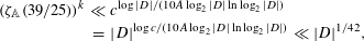 $$\begin{eqnarray}\displaystyle (\unicode[STIX]{x1D701}_{\mathbb{A}}(39/25))^{k} & \ll & \displaystyle c^{\log |D|/(10A\log _{2}|D|\ln \log _{2}|D|)}\nonumber\\ \displaystyle & = & \displaystyle |D|^{\log c/(10A\log _{2}|D|\ln \log _{2}|D|)}\ll |D|^{1/42},\nonumber\end{eqnarray}$$
for
 $n$
large enough. Hence, we have the desired result.◻
$n$
large enough. Hence, we have the desired result.◻
3.2 Evaluating
$S_{1}$
: contribution of the square terms

The last step is to understand the main term
 $S_{1}$
. From Lemma 2.4 we have that
$S_{1}$
. From Lemma 2.4 we have that
 $$\begin{eqnarray}\displaystyle S_{1} & = & \displaystyle \biggl(1+O\biggl(\frac{1}{(\log |D|)^{B}}\biggr)\biggr)\biggl(\mathop{\sum }_{\substack{ f\text{ monic} \\ |f|\leqslant |D|^{1/3} \\ P|f\Rightarrow \deg P\leqslant M}}\frac{d_{z}(f^{2})}{|f|^{2}}\biggl(|{\mathcal{H}}_{n}|\cdot \mathop{\prod }_{P\mid f}\biggl(1+\frac{1}{|P|}\biggr)^{-1}\nonumber\\ \displaystyle & & \displaystyle +\,O(\sqrt{|{\mathcal{H}}_{n}|})\biggr)\biggr).\nonumber\end{eqnarray}$$
Estimating this term is where the difficulties lie, and thus enters the random model
 $L(1,\mathbb{X})$
: let
$L(1,\mathbb{X})$
: let
 $\{\mathbb{X}(P)\}$
denote a sequence of independent random variables indexed by
$\{\mathbb{X}(P)\}$
denote a sequence of independent random variables indexed by
 $P\in \mathbb{A}$
an irreducible (prime) element, which takes the values
$P\in \mathbb{A}$
an irreducible (prime) element, which takes the values
 $0,\pm 1$
described as (1.7). The goal of this section is to prove the following Lemma. Theorem 1.1 follows immediately after combining Lemmas 3.5 and 3.6.
$0,\pm 1$
described as (1.7). The goal of this section is to prove the following Lemma. Theorem 1.1 follows immediately after combining Lemmas 3.5 and 3.6.
Lemma 3.5. Let
 $D\in {\mathcal{H}}_{n}$
. Let
$D\in {\mathcal{H}}_{n}$
. Let
 $z\in \mathbb{C}$
be such that
$z\in \mathbb{C}$
be such that
 $|z|\leqslant \log |D|/(260\log _{2}|D|\ln \log _{2}|D|)$
. Then
$|z|\leqslant \log |D|/(260\log _{2}|D|\ln \log _{2}|D|)$
. Then
 $$\begin{eqnarray}\frac{1}{|{\mathcal{H}}_{n}|}\mathop{\sum }_{D\in {\mathcal{H}}_{n}}L(1,\unicode[STIX]{x1D712}_{D})^{z}=\mathbb{E}(L(1,\mathbb{X})^{z})\biggl(1+O\biggl(\frac{1}{(\log |D|)^{11}}\biggr)\biggr).\end{eqnarray}$$
The expectation of
 $\mathbb{X}$
,
$\mathbb{X}$
,
 $\mathbb{E}(\mathbb{X}(P))$
, is zero and
$\mathbb{E}(\mathbb{X}(P))$
, is zero and
 $\mathbb{E}(\mathbb{X}(P)^{2})=|P|/|P|+1$
. We extend the definition of
$\mathbb{E}(\mathbb{X}(P)^{2})=|P|/|P|+1$
. We extend the definition of
 $\mathbb{X}$
to all monic polynomials
$\mathbb{X}$
to all monic polynomials
 $f\in \mathbb{A}$
as in (1.8). Then, since
$f\in \mathbb{A}$
as in (1.8). Then, since
 $\mathbb{X}$
is independent on the primes, if
$\mathbb{X}$
is independent on the primes, if
 $f=P_{1}^{e_{1}}P_{2}^{e_{2}}\cdots P_{s}^{e_{s}}$
we have
$f=P_{1}^{e_{1}}P_{2}^{e_{2}}\cdots P_{s}^{e_{s}}$
we have
 $$\begin{eqnarray}\mathbb{E}(\mathbb{X}(f))=\mathop{\prod }_{i=1}^{s}\mathbb{E}(\mathbb{X}(P_{i})^{e_{i}}).\end{eqnarray}$$
We note that
 $\mathbb{X}(P)^{e_{j}}=\mathbb{X}(P)$
if
$\mathbb{X}(P)^{e_{j}}=\mathbb{X}(P)$
if
 $e_{j}\equiv 1~(\text{mod}\,2)$
and
$e_{j}\equiv 1~(\text{mod}\,2)$
and
 $\mathbb{X}(P)^{2}$
if
$\mathbb{X}(P)^{2}$
if
 $e_{j}\equiv 0~(\text{mod}\,2)$
. Combining this fact with the independence of
$e_{j}\equiv 0~(\text{mod}\,2)$
. Combining this fact with the independence of
 $\mathbb{X}$
we see that
$\mathbb{X}$
we see that
 $$\begin{eqnarray}\mathbb{E}(\mathbb{X}(P)^{e_{j}})=\left\{\begin{array}{@{}ll@{}}0\quad & \text{if }e_{j}\equiv 1\hspace{0.6em}({\rm mod}\hspace{0.2em}2),\\ \displaystyle \frac{|P|}{|P|+1}\quad & \text{if }e_{j}\equiv 0\hspace{0.6em}({\rm mod}\hspace{0.2em}2).\end{array}\right.\end{eqnarray}$$
Thus, we have proved the following.
Lemma 3.6.
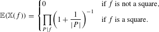 $$\begin{eqnarray}\mathbb{E}(\mathbb{X}(f))=\left\{\begin{array}{@{}ll@{}}0\quad & \text{if }f\text{ is not a square},\\ \displaystyle \mathop{\prod }_{P|f}\biggl(1+\frac{1}{|P|}\biggr)^{-1}\quad & \text{if }f\text{ is a square}.\end{array}\right.\end{eqnarray}$$
Then, for any
 $z\in \mathbb{C}$
since
$z\in \mathbb{C}$
since
 $d_{z}(f)$
and
$d_{z}(f)$
and
 $|f|$
are scalars we see that
$|f|$
are scalars we see that
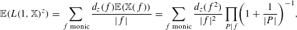 $$\begin{eqnarray}\mathbb{E}(L(1,\mathbb{X})^{z})=\mathop{\sum }_{f\text{ monic}}\frac{d_{z}(f)\mathbb{E}(\mathbb{X}(f))}{|f|}=\mathop{\sum }_{f\text{ monic}}\frac{d_{z}(f^{2})}{|f|^{2}}\mathop{\prod }_{P|f}\biggl(1+\frac{1}{|P|}\biggr)^{-1},\end{eqnarray}$$
where
 $L(1,\mathbb{X})$
is defined in (1.9). We recognize the shape of
$L(1,\mathbb{X})$
is defined in (1.9). We recognize the shape of
 $S_{1}$
from this. On the other hand, from the random Euler product definition we have
$S_{1}$
from this. On the other hand, from the random Euler product definition we have
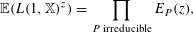 $$\begin{eqnarray}\mathbb{E}(L(1,\mathbb{X})^{z})=\mathop{\prod }_{P\text{ irreducible}}E_{P}(z),\end{eqnarray}$$
where
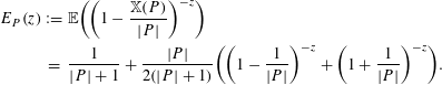 $$\begin{eqnarray}\displaystyle E_{P}(z) & := & \displaystyle \mathbb{E}\biggl(\biggl(1-\frac{\mathbb{X}(P)}{|P|}\biggr)^{-z}\biggr)\nonumber\\ \displaystyle & = & \displaystyle \frac{1}{|P|+1}+\frac{|P|}{2(|P|+1)}\biggl(\biggl(1-\frac{1}{|P|}\biggr)^{-z}+\biggl(1+\frac{1}{|P|}\biggr)^{-z}\biggr).\end{eqnarray}$$
Now, we notice if
 $\deg P>M$
then we can use the following Taylor expansions
$\deg P>M$
then we can use the following Taylor expansions
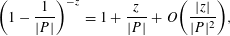 $$\begin{eqnarray}\biggl(1-\frac{1}{|P|}\biggr)^{-z}=1+\frac{z}{|P|}+O\biggl(\frac{|z|}{|P|^{2}}\biggr),\end{eqnarray}$$
and
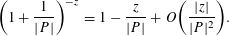 $$\begin{eqnarray}\biggl(1+\frac{1}{|P|}\biggr)^{-z}=1-\frac{z}{|P|}+O\biggl(\frac{|z|}{|P|^{2}}\biggr).\end{eqnarray}$$
That is to say, for
 $P$
irreducible and
$P$
irreducible and
 $\deg P>M$
we have
$\deg P>M$
we have
 $E_{P}(z)=1+O(|z|/|P|^{2})$
, so that
$E_{P}(z)=1+O(|z|/|P|^{2})$
, so that
 $$\begin{eqnarray}\mathop{\prod }_{\substack{ P\text{ irreducible} \\ \deg P>M}}E_{P}(z)\ll \exp \biggl(|z|\mathop{\sum }_{\deg P>M}\frac{1}{|P|^{2}}\biggr)=1+O\biggl(\frac{1}{(\log |D|)^{B}}\biggr),\end{eqnarray}$$
this last equality follows from the relative sizes of
 $|z|$
and
$|z|$
and
 $M$
, where we again note that
$M$
, where we again note that
 $M=A\log _{2}|D|$
and we choose
$M=A\log _{2}|D|$
and we choose
 $A$
large enough to provide the desired error term above. Finally, we use Lemma 3.2 on (3.5), split into sums over square and non-square terms and apply Lemma 3.6 to obtain
$A$
large enough to provide the desired error term above. Finally, we use Lemma 3.2 on (3.5), split into sums over square and non-square terms and apply Lemma 3.6 to obtain
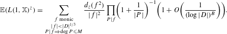 $$\begin{eqnarray}\mathbb{E}(L(1,\mathbb{X})^{z})=\mathop{\sum }_{\substack{ f\text{ monic} \\ |f|<|D|^{1/3} \\ P|f\Rightarrow \deg P\leqslant M}}\frac{d_{z}(f^{2})}{|f|^{2}}\mathop{\prod }_{P|f}\biggl(1+\frac{1}{|P|}\biggr)^{-1}\biggl(1+O\biggl(\frac{1}{(\log |D|)^{B}}\biggr)\biggr).\end{eqnarray}$$
The above discussion and taking the choice
 $A=26$
in Lemma 3.1 gives
$A=26$
in Lemma 3.1 gives
 $B=11$
, which proves Lemma 3.5. Using the fact that
$B=11$
, which proves Lemma 3.5. Using the fact that
 $|D|=q^{n}$
we obtain Theorem 1.1. Corollary 1.7 also follows from this discussion by simply scaling everything appropriately via (1.3) and the fact that expectation is linear. Finally, Corollary 1.9 is obtained in the same way but instead we apply (1.15).
$|D|=q^{n}$
we obtain Theorem 1.1. Corollary 1.7 also follows from this discussion by simply scaling everything appropriately via (1.3) and the fact that expectation is linear. Finally, Corollary 1.9 is obtained in the same way but instead we apply (1.15).
4 The distribution of values of
$L(1,\mathbb{X})$

Here we aim to prove results about
 $\unicode[STIX]{x1D6F7}_{\mathbb{X}}(\unicode[STIX]{x1D70F})$
and
$\unicode[STIX]{x1D6F7}_{\mathbb{X}}(\unicode[STIX]{x1D70F})$
and
 $\unicode[STIX]{x1D6F9}_{\mathbb{X}}(\unicode[STIX]{x1D70F})$
. The proofs of
$\unicode[STIX]{x1D6F9}_{\mathbb{X}}(\unicode[STIX]{x1D70F})$
. The proofs of
 $\unicode[STIX]{x1D6F9}_{\mathbb{X}}(\unicode[STIX]{x1D70F})$
require only minor adjustments to those for
$\unicode[STIX]{x1D6F9}_{\mathbb{X}}(\unicode[STIX]{x1D70F})$
require only minor adjustments to those for
 $\unicode[STIX]{x1D6F7}_{\mathbb{X}}(\unicode[STIX]{x1D70F})$
. The discussion in this section is modelled after [Reference Dahl and Lamzouri6, §4]. These authors use a saddle-point analysis to achieve their results, and we adapt that idea here. To this end, we define some useful auxiliary functions. For
$\unicode[STIX]{x1D6F7}_{\mathbb{X}}(\unicode[STIX]{x1D70F})$
. The discussion in this section is modelled after [Reference Dahl and Lamzouri6, §4]. These authors use a saddle-point analysis to achieve their results, and we adapt that idea here. To this end, we define some useful auxiliary functions. For
 $z\in \mathbb{C}$
define
$z\in \mathbb{C}$
define
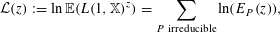 $$\begin{eqnarray}{\mathcal{L}}(z):=\ln \mathbb{E}(L(1,\mathbb{X})^{z})=\mathop{\sum }_{P\text{ irreducible}}\ln (E_{P}(z)),\end{eqnarray}$$
where
 $E_{P}(z)$
is defined as in (3.6). Furthermore, we consider the equation
$E_{P}(z)$
is defined as in (3.6). Furthermore, we consider the equation
 $$\begin{eqnarray}(\mathbb{E}(L(1,\mathbb{X})^{r})(\text{e}^{\unicode[STIX]{x1D6FE}}\unicode[STIX]{x1D70F})^{-r})^{\prime }=0\Leftrightarrow {\mathcal{L}}^{\prime }(r)=\ln (\unicode[STIX]{x1D70F})+\unicode[STIX]{x1D6FE},\end{eqnarray}$$
where the derivative is taken with respect to the real variable
 $r$
. It follows from Proposition 4.2 that
$r$
. It follows from Proposition 4.2 that
 $\lim _{r\rightarrow \infty }{\mathcal{L}}^{\prime }(r)=\infty$
, one can easily check that
$\lim _{r\rightarrow \infty }{\mathcal{L}}^{\prime }(r)=\infty$
, one can easily check that
 $E_{P}^{\prime \prime }(r)E_{P}(r)>(E_{P}^{\prime }(r))^{2}$
for all monic irreducible polynomials
$E_{P}^{\prime \prime }(r)E_{P}(r)>(E_{P}^{\prime }(r))^{2}$
for all monic irreducible polynomials
 $P$
, and thus
$P$
, and thus
 ${\mathcal{L}}^{\prime \prime }(r)>0$
. Therefore, (4.2) has a unique solution: we define
${\mathcal{L}}^{\prime \prime }(r)>0$
. Therefore, (4.2) has a unique solution: we define
 $\unicode[STIX]{x1D705}=\unicode[STIX]{x1D705}(\unicode[STIX]{x1D70F})$
as this unique solution.
$\unicode[STIX]{x1D705}=\unicode[STIX]{x1D705}(\unicode[STIX]{x1D70F})$
as this unique solution.
Finally, we define
 $$\begin{eqnarray}f(t):=\left\{\begin{array}{@{}ll@{}}\ln \cosh (t)\quad & \text{if }0\leqslant t<1,\\ \ln \cosh (t)-t\quad & \text{if }t\geqslant 1.\end{array}\right.\end{eqnarray}$$
4.1 Distribution of the random model
Theorem 4.1. Let
 $\unicode[STIX]{x1D70F}$
be large and
$\unicode[STIX]{x1D70F}$
be large and
 $\unicode[STIX]{x1D705}$
denote the unique solution to (4.2). Then, we have
$\unicode[STIX]{x1D705}$
denote the unique solution to (4.2). Then, we have
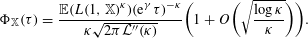 $$\begin{eqnarray}\unicode[STIX]{x1D6F7}_{\mathbb{X}}(\unicode[STIX]{x1D70F})=\frac{\mathbb{E}(L(1,\mathbb{X})^{\unicode[STIX]{x1D705}})(\text{e}^{\unicode[STIX]{x1D6FE}}\unicode[STIX]{x1D70F})^{-\unicode[STIX]{x1D705}}}{\unicode[STIX]{x1D705}\sqrt{2\unicode[STIX]{x1D70B}{\mathcal{L}}^{\prime \prime }(\unicode[STIX]{x1D705})}}\biggl(1+O\biggl(\sqrt{\frac{\log \unicode[STIX]{x1D705}}{\unicode[STIX]{x1D705}}}\biggr)\biggr).\end{eqnarray}$$
Moreover, for any
 $0\leqslant \unicode[STIX]{x1D706}\leqslant 1/\unicode[STIX]{x1D705}$
we have
$0\leqslant \unicode[STIX]{x1D706}\leqslant 1/\unicode[STIX]{x1D705}$
we have
 $$\begin{eqnarray}\unicode[STIX]{x1D6F7}_{\mathbb{X}}(\text{e}^{-\unicode[STIX]{x1D706}}\unicode[STIX]{x1D70F})=\unicode[STIX]{x1D6F7}_{\mathbb{ X}}(\unicode[STIX]{x1D70F})(1+O(\unicode[STIX]{x1D706}\unicode[STIX]{x1D705})).\end{eqnarray}$$
We prove Theorem 1.3 from this and the following proposition, which gives some estimates on the size of
 ${\mathcal{L}}$
and its first few derivatives.
${\mathcal{L}}$
and its first few derivatives.
Proposition 4.2. Let
 $f$
be defined by (4.3). Let
$f$
be defined by (4.3). Let
 $c_{q}\geqslant q$
be a positive constant depending on
$c_{q}\geqslant q$
be a positive constant depending on
 $q$
and let
$q$
and let
 $k\in \mathbb{Z}$
be the unique positive integer such that
$k\in \mathbb{Z}$
be the unique positive integer such that
 $q^{k}\leqslant r<q^{k+1}$
and let
$q^{k}\leqslant r<q^{k+1}$
and let
 $t:=r/q^{k}$
. With this notation in mind for
$t:=r/q^{k}$
. With this notation in mind for
 $r$
any real number such that
$r$
any real number such that
 $r\geqslant c_{q}$
we have
$r\geqslant c_{q}$
we have
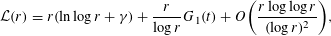 $$\begin{eqnarray}{\mathcal{L}}(r)=r(\ln \log r+\unicode[STIX]{x1D6FE})+\frac{r}{\log r}G_{1}(t)+O\biggl(\frac{r\log \log r}{(\log r)^{2}}\biggr),\end{eqnarray}$$
where
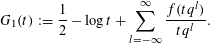 $$\begin{eqnarray}G_{1}(t):=\frac{1}{2}-\log t+\mathop{\sum }_{l=-\infty }^{\infty }\frac{f(tq^{l})}{tq^{l}}.\end{eqnarray}$$
Furthermore, we have
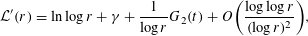 $$\begin{eqnarray}{\mathcal{L}}^{\prime }(r)=\ln \log r+\unicode[STIX]{x1D6FE}+\frac{1}{\log r}G_{2}(t)+O\biggl(\frac{\log \log r}{(\log r)^{2}}\biggr),\end{eqnarray}$$
where
 $$\begin{eqnarray}G_{2}(t):=\frac{1}{2}-\log t+\mathop{\sum }_{l=-\infty }^{\infty }f^{\prime }(tq^{l}).\end{eqnarray}$$
Moreover, for all real numbers
 $y$
,
$y$
,
 $x$
such that
$x$
such that
 $|y|\geqslant c_{q}$
and for all
$|y|\geqslant c_{q}$
and for all
 $x$
such that
$x$
such that
 $|y|\leqslant |x|$
we have
$|y|\leqslant |x|$
we have
 $$\begin{eqnarray}{\mathcal{L}}^{\prime \prime }(y)\asymp \frac{1}{|y|\ln |y|}\quad \text{and}\quad {\mathcal{L}}^{\prime \prime \prime }(y+\text{i}x)\ll \frac{1}{|y|^{2}\ln |y|}.\end{eqnarray}$$
Combining these results gives Theorem 1.3.
Proof of Theorem 1.3.
By Theorem 4.1 and (4.8) we have
 $$\begin{eqnarray}\displaystyle \unicode[STIX]{x1D6F7}_{\mathbb{X}}(\unicode[STIX]{x1D70F}) & = & \displaystyle \frac{\mathbb{E}(L(1,\mathbb{X})^{\unicode[STIX]{x1D705}})(\text{e}^{\unicode[STIX]{x1D6FE}}\unicode[STIX]{x1D70F})^{-\unicode[STIX]{x1D705}}}{\unicode[STIX]{x1D705}\sqrt{2\unicode[STIX]{x1D70B}{\mathcal{L}}^{\prime \prime }(\unicode[STIX]{x1D705})}}\biggl(1+O\biggl(\sqrt{\frac{\log \unicode[STIX]{x1D705}}{\unicode[STIX]{x1D705}}}\biggr)\biggr)\nonumber\\ \displaystyle & = & \displaystyle \exp ({\mathcal{L}}(\unicode[STIX]{x1D705})-\unicode[STIX]{x1D705}(\ln \unicode[STIX]{x1D70F}+\unicode[STIX]{x1D6FE})+O(\log \unicode[STIX]{x1D705})),\nonumber\end{eqnarray}$$
where
 $\unicode[STIX]{x1D705}$
is the unique solution, which satisfies (4.2).
$\unicode[STIX]{x1D705}$
is the unique solution, which satisfies (4.2).
Also from (4.8) we have
 $$\begin{eqnarray}\ln \unicode[STIX]{x1D70F}=\ln \log \unicode[STIX]{x1D705}+\frac{G_{2}(q^{\{\log \unicode[STIX]{x1D705}\}})}{\log \unicode[STIX]{x1D705}}+O\biggl(\frac{\log \log \unicode[STIX]{x1D705}}{(\log \unicode[STIX]{x1D705})^{2}}\biggr).\end{eqnarray}$$
Hence, using (4.6) we obtain
 $$\begin{eqnarray}\unicode[STIX]{x1D6F7}_{\mathbb{X}}(\unicode[STIX]{x1D70F})=\exp \biggl(\unicode[STIX]{x1D705}\frac{G_{1}(q^{\{\log \unicode[STIX]{x1D705}\}})-G_{2}(q^{\{\log \unicode[STIX]{x1D705}\}})}{\log \unicode[STIX]{x1D705}}+O\biggl(\frac{\unicode[STIX]{x1D705}\log \log \unicode[STIX]{x1D705}}{(\log \unicode[STIX]{x1D705})^{2}}\biggr)\biggr).\end{eqnarray}$$
We note that from (4.11), we have
 $\unicode[STIX]{x1D705}\asymp q^{\unicode[STIX]{x1D70F}}$
and thus
$\unicode[STIX]{x1D705}\asymp q^{\unicode[STIX]{x1D70F}}$
and thus
 $$\begin{eqnarray}\log \unicode[STIX]{x1D705}=\unicode[STIX]{x1D70F}-G_{2}(q^{\{\log \unicode[STIX]{x1D705}\}})+O\biggl(\frac{\log \unicode[STIX]{x1D70F}}{\unicode[STIX]{x1D70F}}\biggr),\end{eqnarray}$$
since for every
 $\unicode[STIX]{x1D70F}$
there is a unique
$\unicode[STIX]{x1D70F}$
there is a unique
 $\unicode[STIX]{x1D705}$
, which satisfies (4.2) and
$\unicode[STIX]{x1D705}$
, which satisfies (4.2) and
 $G_{2}(q^{\{\log \unicode[STIX]{x1D705}\}})$
is bounded for any
$G_{2}(q^{\{\log \unicode[STIX]{x1D705}\}})$
is bounded for any
 $\unicode[STIX]{x1D705}$
. This is enough to obtain the shape of the result. It remains to prove that
$\unicode[STIX]{x1D705}$
. This is enough to obtain the shape of the result. It remains to prove that
 $$\begin{eqnarray}\displaystyle -\frac{1}{\ln q}+\frac{\ln \cosh c}{c}-\tanh c & {<} & \displaystyle G_{1}(q^{\{\log \unicode[STIX]{x1D705}\}})-G_{2}(q^{\{\log \unicode[STIX]{x1D705}\}})\nonumber\\ \displaystyle & {<} & \displaystyle \frac{\ln (\cosh (q))}{q}-\tanh (q),\nonumber\end{eqnarray}$$
where
 $c=1.28377\ldots .$
For ease of notation let
$c=1.28377\ldots .$
For ease of notation let
 $t=q^{\{\log \unicode[STIX]{x1D705}\}}$
, we note that
$t=q^{\{\log \unicode[STIX]{x1D705}\}}$
, we note that
 $1\leqslant t<q$
and
$1\leqslant t<q$
and
 $$\begin{eqnarray}G_{1}(t)-G_{2}(t)=\mathop{\sum }_{l=-\infty }^{\infty }\biggl(\frac{f(tq^{l})}{tq^{l}}-f^{\prime }(tq^{l})\biggr).\end{eqnarray}$$
We recall from the definition of
 $f$
that the shape is different depending on the size of the input. So we split the sum:
$f$
that the shape is different depending on the size of the input. So we split the sum:
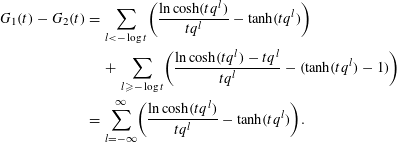 $$\begin{eqnarray}\displaystyle G_{1}(t)-G_{2}(t) & = & \displaystyle \mathop{\sum }_{l<-\log t}\biggl(\frac{\ln \cosh (tq^{l})}{tq^{l}}-\tanh (tq^{l})\biggr)\nonumber\\ \displaystyle & & \displaystyle +\,\mathop{\sum }_{l\geqslant -\log t}\biggl(\frac{\ln \cosh (tq^{l})-tq^{l}}{tq^{l}}-(\tanh (tq^{l})-1)\biggr)\nonumber\\ \displaystyle & = & \displaystyle \mathop{\sum }_{l=-\infty }^{\infty }\biggl(\frac{\ln \cosh (tq^{l})}{tq^{l}}-\tanh (tq^{l})\biggr).\nonumber\end{eqnarray}$$
To prove the upper bound, it is enough to show that all the summands are negative and so the sum will be less than the contribution from the
 $l=0$
term. We note that
$l=0$
term. We note that
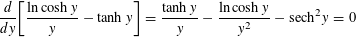 $$\begin{eqnarray}\frac{d}{dy}\biggl[\frac{\ln \cosh y}{y}-\tanh y\biggr]=\frac{\tanh y}{y}-\frac{\ln \cosh y}{y^{2}}-\text{sech}^{2}y=0\end{eqnarray}$$
when
 $y=\pm 1.28377\ldots$
but the argument of our function is
$y=\pm 1.28377\ldots$
but the argument of our function is
 $tq^{l}>0$
for all
$tq^{l}>0$
for all
 $l$
since
$l$
since
 $t,q>0$
, so we need only consider
$t,q>0$
, so we need only consider
 $c=1.28377\ldots .$
A simple calculation shows that this is a minimum and that
$c=1.28377\ldots .$
A simple calculation shows that this is a minimum and that
 $(\ln \cosh y)/y-\tanh y$
is strictly decreasing on the interval
$(\ln \cosh y)/y-\tanh y$
is strictly decreasing on the interval
 $(0,c)$
and strictly increasing on the interval
$(0,c)$
and strictly increasing on the interval
 $(c,\infty )$
. Taking the limit as
$(c,\infty )$
. Taking the limit as
 $y\rightarrow 0$
and
$y\rightarrow 0$
and
 $y\rightarrow \infty$
we see these are both
$y\rightarrow \infty$
we see these are both
 $0$
, and hence all of the summands are negative since
$0$
, and hence all of the summands are negative since
 $(\ln \cosh c)/c-\tanh c=-0.339834\ldots .$
Therefore, we have a suitable upper bound by simply evaluating
$(\ln \cosh c)/c-\tanh c=-0.339834\ldots .$
Therefore, we have a suitable upper bound by simply evaluating
 $(\ln \cosh tq^{l})/tq^{l}-\tanh tq^{l}$
at
$(\ln \cosh tq^{l})/tq^{l}-\tanh tq^{l}$
at
 $l=0$
, which gives
$l=0$
, which gives
 $(\ln \cosh t)/t-\tanh t$
. As we discussed this function reaches its maximum value when
$(\ln \cosh t)/t-\tanh t$
. As we discussed this function reaches its maximum value when
 $t$
does, in this case
$t$
does, in this case
 $t<q$
.
$t<q$
.
In order to consider the lower bound, we note that
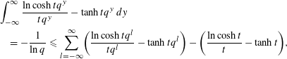 $$\begin{eqnarray}\displaystyle & & \displaystyle \int _{-\infty }^{\infty }\frac{\ln \cosh tq^{y}}{tq^{y}}-\tanh tq^{y}\,dy\nonumber\\ \displaystyle & & \displaystyle \quad =-\frac{1}{\ln q}\leqslant \mathop{\sum }_{l=-\infty }^{\infty }\biggl(\frac{\ln \cosh tq^{l}}{tq^{l}}-\tanh tq^{l}\biggr)-\biggl(\frac{\ln \cosh t}{t}-\tanh t\biggr),\nonumber\end{eqnarray}$$
and hence
 $$\begin{eqnarray}\mathop{\sum }_{l=-\infty }^{\infty }\frac{\ln \cosh tq^{l}}{tq^{l}}-\tanh tq^{l}\geqslant -\frac{1}{\ln q}+\frac{\ln \cosh t}{t}-\tanh t.\end{eqnarray}$$
Finally, as we discussed this is minimized when
 $t=c$
.◻
$t=c$
.◻
4.1.1 Tools for proving Proposition 4.2
First we recall the following standard estimates on
 $f$
and
$f$
and
 $f^{\prime }$
.
$f^{\prime }$
.
Lemma 4.3 [Reference Lamzouri13, Lemma 4.5].
 $f$
is bounded on
$f$
is bounded on
 $[0,\infty )$
and
$[0,\infty )$
and
 $f(t)=t^{2}/2+O(t^{4})$
if
$f(t)=t^{2}/2+O(t^{4})$
if
 $0\leqslant t<1$
. Moreover, we have
$0\leqslant t<1$
. Moreover, we have
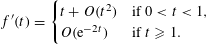 $$\begin{eqnarray}f^{\prime }(t)=\left\{\begin{array}{@{}ll@{}}t+O(t^{2})\quad & \text{if }0<t<1,\\ O(\text{e}^{-2t})\quad & \text{if }t\geqslant 1.\end{array}\right.\end{eqnarray}$$
Lemma 4.4. Let
 $r\geqslant c_{q}$
be a real number, where
$r\geqslant c_{q}$
be a real number, where
 $c_{q}$
is a positive constant depending on
$c_{q}$
is a positive constant depending on
 $q$
. Then we have
$q$
. Then we have
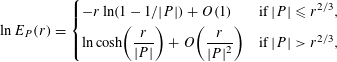 $$\begin{eqnarray}\ln E_{P}(r)=\left\{\begin{array}{@{}ll@{}}\displaystyle -r\ln (1-1/|P|)+O(1)\quad & \text{if }|P|\leqslant r^{2/3},\\ \displaystyle \ln \cosh \biggl(\frac{r}{|P|}\biggr)+O\biggl(\frac{r}{|P|^{2}}\biggr)\quad & \text{if }|P|>r^{2/3},\end{array}\right.\end{eqnarray}$$
and
 $$\begin{eqnarray}\frac{E_{P}^{\prime }}{E_{P}}(r)=\left\{\begin{array}{@{}ll@{}}\displaystyle -\text{ln}\biggl(1-\frac{1}{|P|}\biggr)(1+O(\text{e}^{-r^{1/3}}))\quad & \text{if }|P|\leqslant r^{2/3},\\ \displaystyle \frac{1}{|P|}\tanh \biggl(\frac{r}{|P|}\biggr)+O\biggl(\frac{1}{|P|^{2}}+\frac{r}{|P|^{3}}\biggr)\quad & \text{if }|P|>r^{2/3}.\end{array}\right.\end{eqnarray}$$
Proof. First we prove (4.12). Start by considering
 $|P|\leqslant r^{2/3}$
. Since
$|P|\leqslant r^{2/3}$
. Since
 $|P|$
is small we have
$|P|$
is small we have
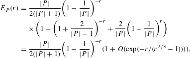 $$\begin{eqnarray}\displaystyle E_{P}(r) & = & \displaystyle \frac{|P|}{2(|P|+1)}\biggl(1-\frac{1}{|P|}\biggr)^{-r}\nonumber\\ \displaystyle & & \displaystyle \times \,\biggl(1+\biggl(1+\frac{2}{|P|-1}\biggr)^{-r}+\frac{2}{|P|}\biggl(1-\frac{1}{|P|}\biggr)^{r}\biggr)\nonumber\\ \displaystyle & = & \displaystyle \frac{|P|}{2(|P|+1)}\biggl(1-\frac{1}{|P|}\biggr)^{-r}(1+O(\exp (-r/(r^{2/3}-1)))),\qquad\end{eqnarray}$$
where the bound in the big
 $O$
comes from Taylor expansion. The final result is obtained by taking logs.
$O$
comes from Taylor expansion. The final result is obtained by taking logs.
Suppose now that
 $|P|>r^{2/3}$
, we see that
$|P|>r^{2/3}$
, we see that
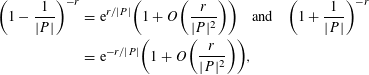 $$\begin{eqnarray}\displaystyle \biggl(1-\frac{1}{|P|}\biggr)^{-r} & = & \displaystyle \text{e}^{r/|P|}\biggl(1+O\biggl(\frac{r}{|P|^{2}}\biggr)\biggr)\quad \text{and}\quad \biggl(1+\frac{1}{|P|}\biggr)^{-r}\nonumber\\ \displaystyle & = & \displaystyle \text{e}^{-r/|P|}\biggl(1+O\biggl(\frac{r}{|P|^{2}}\biggr)\biggr),\nonumber\end{eqnarray}$$
and thus using the bounds
 $\cosh (t)-1\ll t\cosh (t)$
and
$\cosh (t)-1\ll t\cosh (t)$
and
 $\sinh (t)\ll t\cosh (t)$
, which are valid for all
$\sinh (t)\ll t\cosh (t)$
, which are valid for all
 $t\geqslant 0$
we see that
$t\geqslant 0$
we see that
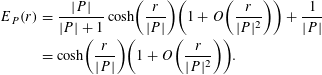 $$\begin{eqnarray}\displaystyle E_{P}(r) & = & \displaystyle \frac{|P|}{|P|+1}\cosh \biggl(\frac{r}{|P|}\biggr)\biggl(1+O\biggl(\frac{r}{|P|^{2}}\biggr)\biggr)+\frac{1}{|P|}\nonumber\\ \displaystyle & = & \displaystyle \cosh \biggl(\frac{r}{|P|}\biggr)\biggl(1+O\biggl(\frac{r}{|P|^{2}}\biggr)\biggr).\end{eqnarray}$$
Taking logs completes the proof.
For (4.13), we first see from (3.6) that
 $$\begin{eqnarray}E_{P}^{\prime }(r)=\frac{-|P|}{2(|P|+1)}\biggl(\biggl(1-\frac{1}{|P|}\biggr)^{-r}\ln \biggl(1-\frac{1}{|P|}\biggr)+\biggl(1+\frac{1}{|P|}\biggr)^{-r}\ln \biggl(1+\frac{1}{|P|}\biggr)\biggr).\end{eqnarray}$$
If
 $|P|\leqslant r^{2/3}$
then (4.14) finishes the claim.
$|P|\leqslant r^{2/3}$
then (4.14) finishes the claim.
On the other hand, for
 $|P|>r^{2/3}$
we have
$|P|>r^{2/3}$
we have
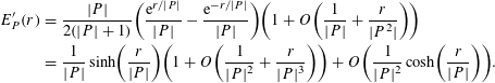 $$\begin{eqnarray}\displaystyle E_{P}^{\prime }(r) & = & \displaystyle \frac{|P|}{2(|P|+1)}\biggl(\frac{\text{e}^{r/|P|}}{|P|}-\frac{\text{e}^{-r/|P|}}{|P|}\biggr)\biggl(1+O\biggl(\frac{1}{|P|}+\frac{r}{|P^{2}|}\biggr)\biggr)\nonumber\\ \displaystyle & = & \displaystyle \frac{1}{|P|}\sinh \biggl(\frac{r}{|P|}\biggr)\biggl(1+O\biggl(\frac{1}{|P|^{2}}+\frac{r}{|P|^{3}}\biggr)\biggr)+O\biggl(\frac{1}{|P|^{2}}\cosh \biggl(\frac{r}{|P|}\biggr)\biggr).\nonumber\end{eqnarray}$$
Combining this with (4.15) we have the desired result. ◻
Proof of Proposition 4.2.
We only write the details for (4.6) and (4.8) as the argument for (4.10) follows along the same lines. For the entire proof, we recall that
 $k\in \mathbb{Z}$
is the unique positive integer such that
$k\in \mathbb{Z}$
is the unique positive integer such that
 $q^{k}\leqslant r<q^{k+1}$
and let
$q^{k}\leqslant r<q^{k+1}$
and let
 $t:=r/q^{k}$
.
$t:=r/q^{k}$
.
We first prove the result for
 ${\mathcal{L}}(r)$
. By Lemmas 4.4 and 4.3 we have
${\mathcal{L}}(r)$
. By Lemmas 4.4 and 4.3 we have
 $$\begin{eqnarray}\displaystyle {\mathcal{L}}(r) & = & \displaystyle -r\mathop{\sum }_{|P|\leqslant r^{2/3}}\ln \biggl(1-\frac{1}{|P|}\biggr)+\mathop{\sum }_{|P|>r^{2/3}}\ln \cosh \biggl(\frac{r}{|P|}\biggr)+O(r^{2/3})\nonumber\\ \displaystyle & = & \displaystyle -r\mathop{\sum }_{\deg P\leqslant k}\ln \biggl(1-\frac{1}{|P|}\biggr)+\mathop{\sum }_{|P|>r^{2/3}}f\biggl(\frac{r}{|P|}\biggr)+O(r^{2/3}).\end{eqnarray}$$
The first summand is taken care of by recognizing Mertens’ theorem, which we will apply at the end. The more interesting part of the proof comes from the second sum. First, from the prime number theorem we get
 $$\begin{eqnarray}\mathop{\sum }_{|P|>r^{2/3}}f\biggl(\frac{r}{|P|}\biggr)=\mathop{\sum }_{n>(2/3)\log r}\frac{q^{n}}{n}f\biggl(\frac{r}{q^{n}}\biggr)+O\biggl(\mathop{\sum }_{n>(2/3)\log r}\frac{q^{n/2}}{n}f\biggl(\frac{r}{q^{n}}\biggr)\biggr).\end{eqnarray}$$
The error term is
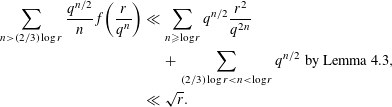 $$\begin{eqnarray}\displaystyle \mathop{\sum }_{n>(2/3)\log r}\frac{q^{n/2}}{n}f\biggl(\frac{r}{q^{n}}\biggr) & \ll & \displaystyle \mathop{\sum }_{n\geqslant \log r}q^{n/2}\frac{r^{2}}{q^{2n}}\nonumber\\ \displaystyle & & \displaystyle +\,\mathop{\sum }_{(2/3)\log r<n<\log r}q^{n/2}\text{ by Lemma 4.3},\nonumber\\ \displaystyle & \ll & \displaystyle \sqrt{r}.\nonumber\end{eqnarray}$$
It remains to consider
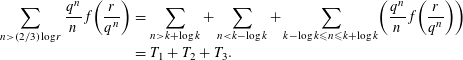 $$\begin{eqnarray}\displaystyle \!\mathop{\sum }_{n>(2/3)\log r}\frac{q^{n}}{n}f\biggl(\frac{r}{q^{n}}\biggr) & = & \displaystyle \mathop{\sum }_{n>k+\log k}+\mathop{\sum }_{n<k-\log k}+\mathop{\sum }_{k-\log k\leqslant n\leqslant k+\log k}\biggl(\frac{q^{n}}{n}f\biggl(\frac{r}{q^{n}}\biggr)\biggr)\nonumber\\ \displaystyle & = & \displaystyle T_{1}+T_{2}+T_{3}.\nonumber\end{eqnarray}$$
We first bound
 $T_{1}$
and
$T_{1}$
and
 $T_{2}$
, again referring to Lemma 4.3
$T_{2}$
, again referring to Lemma 4.3
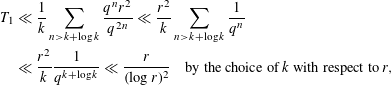 $$\begin{eqnarray}\displaystyle T_{1} & \ll & \displaystyle \frac{1}{k}\mathop{\sum }_{n>k+\log k}\frac{q^{n}r^{2}}{q^{2n}}\ll \frac{r^{2}}{k}\mathop{\sum }_{n>k+\log k}\frac{1}{q^{n}}\nonumber\\ \displaystyle & \ll & \displaystyle \frac{r^{2}}{k}\frac{1}{q^{k+\log k}}\ll \frac{r}{(\log r)^{2}}\quad \text{by the choice of }k\text{ with respect to }r,\nonumber\end{eqnarray}$$
and similarly
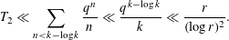 $$\begin{eqnarray}T_{2}\ll \mathop{\sum }_{n<k-\log k}\frac{q^{n}}{n}\ll \frac{q^{k-\log k}}{k}\ll \frac{r}{(\log r)^{2}}.\end{eqnarray}$$
For
 $T_{3}$
we notice that for
$T_{3}$
we notice that for
 $n\in [k-\log k,k+\log k]$
, we have
$n\in [k-\log k,k+\log k]$
, we have
 $1/n=(1/k)(1+O(\ln k/k))$
. Using this, we factor out
$1/n=(1/k)(1+O(\ln k/k))$
. Using this, we factor out
 $q^{k}/k$
and do the variable change
$q^{k}/k$
and do the variable change
 $l=k-n$
so that
$l=k-n$
so that
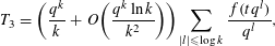 $$\begin{eqnarray}T_{3}=\biggl(\frac{q^{k}}{k}+O\biggl(\frac{q^{k}\ln k}{k^{2}}\biggr)\biggr)\mathop{\sum }_{|l|\leqslant \log k}\frac{f(tq^{l})}{q^{l}},\end{eqnarray}$$
where we recall
 $t:=r/q^{k}$
. Next, we see that for
$t:=r/q^{k}$
. Next, we see that for
 $|l|>\log k$
the sum is small:
$|l|>\log k$
the sum is small:
 $$\begin{eqnarray}\mathop{\sum }_{|l|>\log k}\frac{f(tq^{l})}{q^{l}}\ll \mathop{\sum }_{l>\log k}\frac{1}{q^{l}}+\mathop{\sum }_{l<-\log k}q^{l}\ll \frac{1}{q^{\ln k}}\ll \frac{1}{k}.\end{eqnarray}$$
Hence, we have
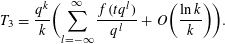 $$\begin{eqnarray}T_{3}=\frac{q^{k}}{k}\biggl(\mathop{\sum }_{l=-\infty }^{\infty }\frac{f(tq^{l})}{q^{l}}+O\biggl(\frac{\ln k}{k}\biggr)\biggr).\end{eqnarray}$$
Returning this to an expression in terms of
 $r$
we see
$r$
we see
 $$\begin{eqnarray}T_{3}=\frac{r}{\log r}\biggl(\mathop{\sum }_{l=-\infty }^{\infty }\frac{f(tq^{l})}{tq^{l}}+O\biggl(\frac{\ln \ln r}{\ln r}\biggr)\biggr).\end{eqnarray}$$
Finally, we complete the bound of
 ${\mathcal{L}}(r)$
by applying Mertens’ theorem to the first summand and convert everything in terms of
${\mathcal{L}}(r)$
by applying Mertens’ theorem to the first summand and convert everything in terms of
 $r$
. Combining the terms that have
$r$
. Combining the terms that have
 $r/\log r$
in common we achieve the claimed result.
$r/\log r$
in common we achieve the claimed result.
For
 ${\mathcal{L}}^{\prime }(r)$
, we again appeal to Lemmas 4.4 and 4.3 giving
${\mathcal{L}}^{\prime }(r)$
, we again appeal to Lemmas 4.4 and 4.3 giving
 $$\begin{eqnarray}\displaystyle {\mathcal{L}}^{\prime }(r) & = & \displaystyle -\mathop{\sum }_{|P|\leqslant r^{2/3}}\ln \biggl(1-\frac{1}{|P|}\biggr)+\mathop{\sum }_{|P|>r^{2/3}}\frac{\tanh (r/|P|)}{|P|}+O(r^{-1/3})\nonumber\\ \displaystyle & = & \displaystyle -\mathop{\sum }_{\deg P\leqslant k}\ln \biggl(1-\frac{1}{|P|}\biggr)+\mathop{\sum }_{|P|>r^{2/3}}\frac{f^{\prime }(r/|P|)}{|P|}+O(r^{-1/3}).\end{eqnarray}$$
Applying the prime number theorem to the second sum we obtain
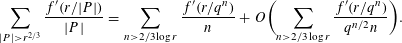 $$\begin{eqnarray}\mathop{\sum }_{|P|>r^{2/3}}\frac{f^{\prime }(r/|P|)}{|P|}=\mathop{\sum }_{n>2/3\log r}\frac{f^{\prime }(r/q^{n})}{n}+O\biggl(\mathop{\sum }_{n>2/3\log r}\frac{f^{\prime }(r/q^{n})}{q^{n/2}n}\biggr).\end{eqnarray}$$
The error term in this case is
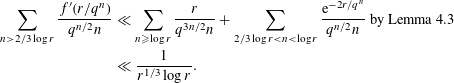 $$\begin{eqnarray}\displaystyle \mathop{\sum }_{n>2/3\log r}\frac{f^{\prime }(r/q^{n})}{q^{n/2}n} & \ll & \displaystyle \mathop{\sum }_{n\geqslant \log r}\frac{r}{q^{3n/2}n}+\mathop{\sum }_{2/3\log r<n<\log r}\frac{\text{e}^{-2r/q^{n}}}{q^{n/2}n}\text{ by Lemma 4.3}\nonumber\\ \displaystyle & \ll & \displaystyle \frac{1}{r^{1/3}\log r}.\nonumber\end{eqnarray}$$
As before, we split the remaining sum into three pieces:
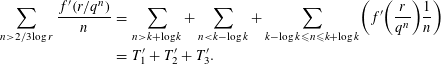 $$\begin{eqnarray}\displaystyle \mathop{\sum }_{n>2/3\log r}\frac{f^{\prime }(r/q^{n})}{n} & = & \displaystyle \mathop{\sum }_{n>k+\log k}+\mathop{\sum }_{n<k-\log k}+\mathop{\sum }_{k-\log k\leqslant n\leqslant k+\log k}\biggl(f^{\prime }\biggl(\frac{r}{q^{n}}\biggr)\frac{1}{n}\biggr)\nonumber\\ \displaystyle & = & \displaystyle T_{1}^{\prime }+T_{2}^{\prime }+T_{3}^{\prime }.\nonumber\end{eqnarray}$$
We first bound
 $T_{1}^{\prime }$
and
$T_{1}^{\prime }$
and
 $T_{2}^{\prime }$
, referring to Lemma 4.3 gives
$T_{2}^{\prime }$
, referring to Lemma 4.3 gives
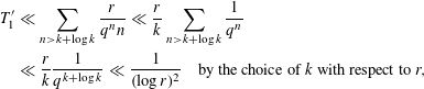 $$\begin{eqnarray}\displaystyle T_{1}^{\prime } & \ll & \displaystyle \mathop{\sum }_{n>k+\log k}\frac{r}{q^{n}n}\ll \frac{r}{k}\mathop{\sum }_{n>k+\log k}\frac{1}{q^{n}}\nonumber\\ \displaystyle & \ll & \displaystyle \frac{r}{k}\frac{1}{q^{k+\log k}}\ll \frac{1}{(\log r)^{2}}\quad \text{by the choice of }k\text{ with respect to }r,\nonumber\end{eqnarray}$$
similarly
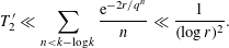 $$\begin{eqnarray}T_{2}^{\prime }\ll \mathop{\sum }_{n<k-\log k}\frac{\text{e}^{-2r/q^{n}}}{n}\ll \frac{1}{(\log r)^{2}}.\end{eqnarray}$$
For
 $T_{3}^{\prime }$
we notice that for
$T_{3}^{\prime }$
we notice that for
 $n\in [k-\log k,k+\log k]$
, we have
$n\in [k-\log k,k+\log k]$
, we have
 $1/n=(1/k)(1+O(\ln k/k))$
. Using this, we factor out
$1/n=(1/k)(1+O(\ln k/k))$
. Using this, we factor out
 $q^{k}/k$
and do the variable change
$q^{k}/k$
and do the variable change
 $l=k-n$
and recall
$l=k-n$
and recall
 $t:=r/q^{k}$
, so that
$t:=r/q^{k}$
, so that
 $$\begin{eqnarray}T_{3}^{\prime }\ll \biggl(\frac{1}{k}+O\biggl(\frac{\ln k}{k^{2}}\biggr)\biggr)\mathop{\sum }_{|l|<\log k}f^{\prime }(tq^{l}).\end{eqnarray}$$
Next, we show this sum is small for
 $|l|>\log k$
:
$|l|>\log k$
:
 $$\begin{eqnarray}\displaystyle \mathop{\sum }_{|l|>\log k}f^{\prime }(tq^{l}) & \ll & \displaystyle \mathop{\sum }_{l>\log k}\text{e}^{-2tq^{l}}+\mathop{\sum }_{l<-\log k}tq^{l}\nonumber\\ \displaystyle & \ll & \displaystyle \text{e}^{-2\log r}+\frac{1}{q^{\log k}},\nonumber\\ \displaystyle & & \displaystyle \text{the bound on the second sum follows from }1\leqslant t\leqslant q\nonumber\\ \displaystyle & \ll & \displaystyle \frac{1}{\log r}.\nonumber\end{eqnarray}$$
Hence, we have
 $$\begin{eqnarray}T_{3}^{\prime }\ll \frac{1}{k}\biggl(\mathop{\sum }_{l=-\infty }^{\infty }f^{\prime }(tq^{l})+O\biggl(\frac{\ln k}{k}\biggr)\biggr).\end{eqnarray}$$
Finally, we complete the bound of
 ${\mathcal{L}}^{\prime }(r)$
by applying Mertens’ theorem to the first summand and convert everything in terms of
${\mathcal{L}}^{\prime }(r)$
by applying Mertens’ theorem to the first summand and convert everything in terms of
 $r$
. Combining the terms that have
$r$
. Combining the terms that have
 $1/\log r$
in common we achieve the claimed result.◻
$1/\log r$
in common we achieve the claimed result.◻
4.1.2 Proof of Theorem 4.1
One of the key ingredients in the proof of Theorem 4.1 is to show that
 $|\mathbb{E}(L(1,\mathbb{X})^{r+\text{i}t})|/\mathbb{E}(L(1,\mathbb{X})^{r})$
is rapidly decreasing in
$|\mathbb{E}(L(1,\mathbb{X})^{r+\text{i}t})|/\mathbb{E}(L(1,\mathbb{X})^{r})$
is rapidly decreasing in
 $t$
when
$t$
when
 $|t|\geqslant \sqrt{r\ln r}$
. For this we prove the following lemmas.
$|t|\geqslant \sqrt{r\ln r}$
. For this we prove the following lemmas.
Lemma 4.5. Let
 $r$
be a large positive number and
$r$
be a large positive number and
 $c_{q}\geqslant q$
a positive constant depending on
$c_{q}\geqslant q$
a positive constant depending on
 $q$
. If
$q$
. If
 $|P|>r/c_{q}$
, then for some positive constant
$|P|>r/c_{q}$
, then for some positive constant
 $b_{1}$
we have
$b_{1}$
we have
 $$\begin{eqnarray}\frac{|E_{P}(r+\text{i}t)|}{E_{P}(r)}\leqslant \exp \biggl(-b_{1}\biggl(1-\cos \biggl(t\ln \biggl(\frac{|P|+1}{|P|-1}\biggr)\biggr)\biggr)\biggr),\end{eqnarray}$$
where
 $c_{q}$
is a positive constant dependent on
$c_{q}$
is a positive constant dependent on
 $q$
.
$q$
.
Proof. Let
 $x_{1}$
,
$x_{1}$
,
 $x_{2}$
and
$x_{2}$
and
 $x_{3}$
be positive real numbers and
$x_{3}$
be positive real numbers and
 $\unicode[STIX]{x1D703}_{2}$
and
$\unicode[STIX]{x1D703}_{2}$
and
 $\unicode[STIX]{x1D703}_{3}$
be real numbers. We use the following inequality established in the proof of [Reference Granville and Soundararajan7, Lemma 3.2]:
$\unicode[STIX]{x1D703}_{3}$
be real numbers. We use the following inequality established in the proof of [Reference Granville and Soundararajan7, Lemma 3.2]:
 $$\begin{eqnarray}|x_{1}+x_{2}\text{e}^{\text{i}\unicode[STIX]{x1D703}_{2}}+x_{3}\text{e}^{\text{i}\unicode[STIX]{x1D703}_{3}}|\leqslant (x_{1}+x_{2}+x_{3})\exp \biggl(-\frac{x_{1}x_{3}(1-\cos \unicode[STIX]{x1D703}_{3})}{(x_{1}+x_{2}+x_{3})^{2}}\biggr).\end{eqnarray}$$
Choosing
 $x_{1}=(|P|/2(|P|+1))(1+1/|P|)^{-r}$
,
$x_{1}=(|P|/2(|P|+1))(1+1/|P|)^{-r}$
,
 $x_{2}=1/(|P|+1)$
and
$x_{2}=1/(|P|+1)$
and
 $x_{3}=(|P|/2(|P|+1))(1-1/|P|)^{-r}$
with
$x_{3}=(|P|/2(|P|+1))(1-1/|P|)^{-r}$
with
 $\unicode[STIX]{x1D703}_{2}=t\ln (1+1/|P|)$
and
$\unicode[STIX]{x1D703}_{2}=t\ln (1+1/|P|)$
and
 $\unicode[STIX]{x1D703}_{3}=t\ln ((|P|+1)/(|P|-1))$
provides the desired result since
$\unicode[STIX]{x1D703}_{3}=t\ln ((|P|+1)/(|P|-1))$
provides the desired result since
 $|P|>r/c_{q}$
.◻
$|P|>r/c_{q}$
.◻
Lemma 4.6. Let
 $r$
be large and let
$r$
be large and let
 $c_{q}\geqslant q>4$
be a positive constant dependent on
$c_{q}\geqslant q>4$
be a positive constant dependent on
 $q$
. Then there exists a constant
$q$
. Then there exists a constant
 $b_{2}>0$
such that
$b_{2}>0$
such that
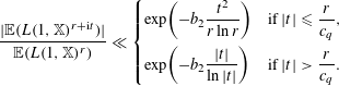 $$\begin{eqnarray}\frac{|\mathbb{E}(L(1,\mathbb{X})^{r+\text{i}t})|}{\mathbb{E}(L(1,\mathbb{X})^{r})}\ll \left\{\begin{array}{@{}ll@{}}\displaystyle \exp \biggl(-b_{2}\frac{t^{2}}{r\ln r}\biggr)\quad & \displaystyle \text{if }|t|\leqslant \frac{r}{c_{q}},\\ \displaystyle \exp \biggl(-b_{2}\frac{|t|}{\ln |t|}\biggr)\quad & \displaystyle \text{if }|t|>\frac{r}{c_{q}}.\end{array}\right.\end{eqnarray}$$
Proof. Let
 $z=r+\text{i}t$
. Since
$z=r+\text{i}t$
. Since
 $|E_{P}(z)|\leqslant E_{P}(r)$
we obtain for any real numbers
$|E_{P}(z)|\leqslant E_{P}(r)$
we obtain for any real numbers
 $q\leqslant y_{1}<y_{2}$
that
$q\leqslant y_{1}<y_{2}$
that
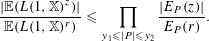 $$\begin{eqnarray}\frac{|\mathbb{E}(L(1,\mathbb{X})^{z})|}{\mathbb{E}(L(1,\mathbb{X})^{r})}\leqslant \mathop{\prod }_{y_{1}\leqslant |P|\leqslant y_{2}}\frac{|E_{P}(z)|}{E_{P}(r)}.\end{eqnarray}$$
Note that
 $|t|\ln (|P|+1/|P|-1)\sim 2|t|/|P|$
so that when
$|t|\ln (|P|+1/|P|-1)\sim 2|t|/|P|$
so that when
 $|t|\leqslant |P|/c_{q}$
we have
$|t|\leqslant |P|/c_{q}$
we have
 $$\begin{eqnarray}1-\cos \biggl(|t|\ln \biggl(\frac{|P|+1}{|P|-1}\biggr)\biggr)\gg \frac{|t|^{2}}{|P|^{2}}.\end{eqnarray}$$
If
 $|t|\leqslant r/c_{q}$
then, we choose
$|t|\leqslant r/c_{q}$
then, we choose
 $y_{1}=r$
and
$y_{1}=r$
and
 $y_{2}=c_{q}r/2$
. Appealing to Lemma 4.5 we have
$y_{2}=c_{q}r/2$
. Appealing to Lemma 4.5 we have
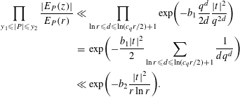 $$\begin{eqnarray}\displaystyle \mathop{\prod }_{y_{1}\leqslant |P|\leqslant y_{2}}\frac{|E_{P}(z)|}{E_{P}(r)} & \ll & \displaystyle \mathop{\prod }_{\ln r\leqslant d\leqslant \ln (c_{q}r/2)+1}\exp \biggl(-b_{1}\frac{q^{d}}{2d}\frac{|t|^{2}}{q^{2d}}\biggr)\nonumber\\ \displaystyle & = & \displaystyle \exp \biggl(-\frac{b_{1}|t|^{2}}{2}\mathop{\sum }_{\ln r\leqslant d\leqslant \ln (c_{q}r/2)+1}\frac{1}{dq^{d}}\biggr)\nonumber\\ \displaystyle & \ll & \displaystyle \exp \biggl(-b_{2}\frac{|t|^{2}}{r\ln r}\biggr).\nonumber\end{eqnarray}$$
In the case of
 $|t|>r/c_{q}$
we use a similar argument but choose
$|t|>r/c_{q}$
we use a similar argument but choose
 $y_{1}=c_{q}|t|$
and
$y_{1}=c_{q}|t|$
and
 $y_{2}=2c_{q}|t|$
to complete the result.◻
$y_{2}=2c_{q}|t|$
to complete the result.◻
Let
 $\unicode[STIX]{x1D711}(y)=1$
if
$\unicode[STIX]{x1D711}(y)=1$
if
 $y>1$
and be equal to
$y>1$
and be equal to
 $0$
otherwise. Then we have the following smooth analogue of Perron’s formula.
$0$
otherwise. Then we have the following smooth analogue of Perron’s formula.
Lemma 4.7 [Reference Dahl and Lamzouri6, Lemma 4.7].
Let
 $\unicode[STIX]{x1D706}>0$
be a real number and
$\unicode[STIX]{x1D706}>0$
be a real number and
 $N$
be a positive integer. For any
$N$
be a positive integer. For any
 $c>0$
we have for
$c>0$
we have for
 $y>0$
$y>0$
 $$\begin{eqnarray}\displaystyle 0 & {\leqslant} & \displaystyle \frac{1}{2\unicode[STIX]{x1D70B}\text{i}}\int _{c-\text{i}\infty }^{c+\text{i}\infty }y^{s}\biggl(\frac{\text{e}^{\unicode[STIX]{x1D706}s}-1}{\unicode[STIX]{x1D706}s}\biggr)^{N}\frac{ds}{s}-\unicode[STIX]{x1D711}(y)\nonumber\\ \displaystyle & {\leqslant} & \displaystyle \frac{1}{2\unicode[STIX]{x1D70B}\text{i}}\int _{c-\text{i}\infty }^{c+\text{i}\infty }y^{s}\biggl(\frac{\text{e}^{\unicode[STIX]{x1D706}s}-1}{\unicode[STIX]{x1D706}s}\biggr)^{N}\frac{1-\text{e}^{-\unicode[STIX]{x1D706}Ns}}{s}\,ds,\end{eqnarray}$$
and
 $$\begin{eqnarray}0\leqslant \unicode[STIX]{x1D711}(\text{e}^{\unicode[STIX]{x1D706}}y)-\unicode[STIX]{x1D711}(y)\leqslant \frac{1}{2\unicode[STIX]{x1D70B}\text{i}}\int _{c-\text{i}\infty }^{c+\text{i}\infty }y^{s}\biggl(\frac{\text{e}^{\unicode[STIX]{x1D706}s}-1}{\unicode[STIX]{x1D706}s}\biggr)\frac{\text{e}^{\unicode[STIX]{x1D706}s}-\text{e}^{-\unicode[STIX]{x1D706}s}}{s}\,ds.\end{eqnarray}$$
Proof of Theorem 4.1.
We first prove (4.4). Let
 $0<\unicode[STIX]{x1D706}<1/(2\unicode[STIX]{x1D705})$
be a real number, which we choose later. Using (4.19) from Lemma 4.7, taking
$0<\unicode[STIX]{x1D706}<1/(2\unicode[STIX]{x1D705})$
be a real number, which we choose later. Using (4.19) from Lemma 4.7, taking
 $N=1$
we obtain
$N=1$
we obtain
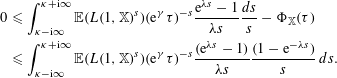 $$\begin{eqnarray}\displaystyle 0 & {\leqslant} & \displaystyle \int _{\unicode[STIX]{x1D705}-\text{i}\infty }^{\unicode[STIX]{x1D705}+\text{i}\infty }\mathbb{E}(L(1,\mathbb{X})^{s})(\text{e}^{\unicode[STIX]{x1D6FE}}\unicode[STIX]{x1D70F})^{-s}\frac{\text{e}^{\unicode[STIX]{x1D706}s}-1}{\unicode[STIX]{x1D706}s}\frac{ds}{s}-\unicode[STIX]{x1D6F7}_{\mathbb{X}}(\unicode[STIX]{x1D70F})\nonumber\\ \displaystyle & {\leqslant} & \displaystyle \int _{\unicode[STIX]{x1D705}-\text{i}\infty }^{\unicode[STIX]{x1D705}+\text{i}\infty }\mathbb{E}(L(1,\mathbb{X})^{s})(\text{e}^{\unicode[STIX]{x1D6FE}}\unicode[STIX]{x1D70F})^{-s}\frac{(\text{e}^{\unicode[STIX]{x1D706}s}-1)}{\unicode[STIX]{x1D706}s}\frac{(1-\text{e}^{-\unicode[STIX]{x1D706}s})}{s}\,ds.\end{eqnarray}$$
Since
 $\unicode[STIX]{x1D706}\unicode[STIX]{x1D705}<1/2$
we have
$\unicode[STIX]{x1D706}\unicode[STIX]{x1D705}<1/2$
we have
 $|\text{e}^{\unicode[STIX]{x1D706}s}-1|\leqslant 3$
and
$|\text{e}^{\unicode[STIX]{x1D706}s}-1|\leqslant 3$
and
 $|\text{e}^{-\unicode[STIX]{x1D706}s}-1|\leqslant 2$
. Hence, using Lemma 4.6 along with the fact that
$|\text{e}^{-\unicode[STIX]{x1D706}s}-1|\leqslant 2$
. Hence, using Lemma 4.6 along with the fact that
 $|\mathbb{E}(L(1,\mathbb{X})^{s})|\leqslant \mathbb{E}(L(1,\mathbb{X})^{\unicode[STIX]{x1D705}})$
we obtain, for some constant
$|\mathbb{E}(L(1,\mathbb{X})^{s})|\leqslant \mathbb{E}(L(1,\mathbb{X})^{\unicode[STIX]{x1D705}})$
we obtain, for some constant
 $b_{3}>0$
that
$b_{3}>0$
that
 $$\begin{eqnarray}\displaystyle & & \displaystyle \int _{\unicode[STIX]{x1D705}-\text{i}\infty }^{\unicode[STIX]{x1D705}-\text{i}\unicode[STIX]{x1D705}^{3/5}}+\int _{\unicode[STIX]{x1D705}+\text{i}\unicode[STIX]{x1D705}^{3/5}}^{\unicode[STIX]{x1D705}+\text{i}\infty }\mathbb{E}(L(1,\mathbb{X})^{s})(\text{e}^{\unicode[STIX]{x1D6FE}}\unicode[STIX]{x1D70F})^{-s}\frac{\text{e}^{\unicode[STIX]{x1D706}s}-1}{\unicode[STIX]{x1D706}s}\frac{ds}{s}\nonumber\\ \displaystyle & & \displaystyle \quad \ll \,\frac{\text{e}^{-b_{3}\unicode[STIX]{x1D705}^{1/6}}}{\unicode[STIX]{x1D706}\unicode[STIX]{x1D705}^{3/5}}\mathbb{E}(L(1,\mathbb{X})^{\unicode[STIX]{x1D705}})(\text{e}^{\unicode[STIX]{x1D6FE}}\unicode[STIX]{x1D70F})^{-\unicode[STIX]{x1D705}},\end{eqnarray}$$
and similarly,
 $$\begin{eqnarray}\displaystyle & & \displaystyle \int _{\unicode[STIX]{x1D705}-\text{i}\infty }^{\unicode[STIX]{x1D705}-\text{i}\unicode[STIX]{x1D705}^{3/5}}+\int _{\unicode[STIX]{x1D705}+\text{i}\unicode[STIX]{x1D705}^{3/5}}^{\unicode[STIX]{x1D705}+\text{i}\infty }\mathbb{E}(L(1,\mathbb{X})^{s})(\text{e}^{\unicode[STIX]{x1D6FE}}\unicode[STIX]{x1D70F})^{-s}\frac{(\text{e}^{\unicode[STIX]{x1D706}s}-1)}{\unicode[STIX]{x1D706}s}\frac{(1-\text{e}^{-\unicode[STIX]{x1D706}s})}{s}\,ds\nonumber\\ \displaystyle & & \displaystyle \quad \ll \,\frac{\text{e}^{-b_{3}\unicode[STIX]{x1D705}^{1/6}}}{\unicode[STIX]{x1D706}\unicode[STIX]{x1D705}^{3/5}}\mathbb{E}(L(1,\mathbb{X})^{\unicode[STIX]{x1D705}})(\text{e}^{\unicode[STIX]{x1D6FE}}\unicode[STIX]{x1D70F})^{-\unicode[STIX]{x1D705}}.\end{eqnarray}$$
Let
 $s=\unicode[STIX]{x1D705}+\text{i}t$
. If
$s=\unicode[STIX]{x1D705}+\text{i}t$
. If
 $|t|\leqslant \unicode[STIX]{x1D705}^{3/5}$
then
$|t|\leqslant \unicode[STIX]{x1D705}^{3/5}$
then
 $|(\text{e}^{\unicode[STIX]{x1D706}s}-1)(1-\text{e}^{-\unicode[STIX]{x1D706}s})|\ll \unicode[STIX]{x1D706}^{2}|s|^{2}$
, and hence the remaining part of the integral is bounded as follows:
$|(\text{e}^{\unicode[STIX]{x1D706}s}-1)(1-\text{e}^{-\unicode[STIX]{x1D706}s})|\ll \unicode[STIX]{x1D706}^{2}|s|^{2}$
, and hence the remaining part of the integral is bounded as follows:
 $$\begin{eqnarray}\displaystyle & & \displaystyle \int _{\unicode[STIX]{x1D705}-\text{i}\unicode[STIX]{x1D705}^{3/5}}^{\unicode[STIX]{x1D705}+\text{i}\unicode[STIX]{x1D705}^{3/5}}\mathbb{E}(L(1,\mathbb{X})^{s})(\text{e}^{\unicode[STIX]{x1D6FE}}\unicode[STIX]{x1D70F})^{-s}\frac{(\text{e}^{\unicode[STIX]{x1D706}s}-1)}{\unicode[STIX]{x1D706}s}\frac{(1-\text{e}^{-\unicode[STIX]{x1D706}s})}{s}\,ds\nonumber\\ \displaystyle & & \displaystyle \quad \ll \,\unicode[STIX]{x1D706}\unicode[STIX]{x1D705}^{3/5}\mathbb{E}(L(1,\mathbb{X})^{\unicode[STIX]{x1D705}})(\text{e}^{\unicode[STIX]{x1D6FE}}\unicode[STIX]{x1D70F})^{-\unicode[STIX]{x1D705}}.\nonumber\end{eqnarray}$$
Combining this estimate with (4.21), (4.22) and (4.23) we obtain
 $$\begin{eqnarray}\displaystyle & & \displaystyle \unicode[STIX]{x1D6F7}_{\mathbb{X}}(\unicode[STIX]{x1D70F})-\frac{1}{2\unicode[STIX]{x1D70B}\text{i}}\int _{\unicode[STIX]{x1D705}-\text{i}\unicode[STIX]{x1D705}^{3/5}}^{\unicode[STIX]{x1D705}+\text{i}\unicode[STIX]{x1D705}^{3/5}}\mathbb{E}(L(1,\mathbb{X})^{s})(\text{e}^{\unicode[STIX]{x1D6FE}}\unicode[STIX]{x1D70F})^{-s}\frac{(\text{e}^{\unicode[STIX]{x1D706}s}-1)}{\unicode[STIX]{x1D706}s^{2}}\,ds\nonumber\\ \displaystyle & & \displaystyle \quad \ll \,\biggl(\unicode[STIX]{x1D706}\unicode[STIX]{x1D705}^{3/5}+\frac{\text{e}^{-b_{3}\unicode[STIX]{x1D705}^{1/6}}}{\unicode[STIX]{x1D706}\unicode[STIX]{x1D705}^{3/5}}\biggr)\mathbb{E}(L(1,\mathbb{X})^{\unicode[STIX]{x1D705}})(\text{e}^{\unicode[STIX]{x1D6FE}}\unicode[STIX]{x1D70F})^{-\unicode[STIX]{x1D705}}.\end{eqnarray}$$
On the other hand, we have from (4.10) when
 $|t|\leqslant \unicode[STIX]{x1D705}^{3/5}$
then
$|t|\leqslant \unicode[STIX]{x1D705}^{3/5}$
then
 $$\begin{eqnarray}{\mathcal{L}}(\unicode[STIX]{x1D705}+\text{i}t)={\mathcal{L}}(\unicode[STIX]{x1D705})+\text{i}t{\mathcal{L}}^{\prime }(\unicode[STIX]{x1D705})-\frac{t^{2}}{2}{\mathcal{L}}^{\prime \prime }(\unicode[STIX]{x1D705})+O\biggl(\frac{|t|^{3}}{\unicode[STIX]{x1D705}^{2}\ln \unicode[STIX]{x1D705}}\biggr).\end{eqnarray}$$
We also note that
 $$\begin{eqnarray}\frac{\text{e}^{\unicode[STIX]{x1D706}s}-1}{\unicode[STIX]{x1D706}s^{2}}=\frac{1}{s}(1+O(\unicode[STIX]{x1D705}))=\frac{1}{\unicode[STIX]{x1D705}}\biggl(1-\text{i}\frac{t}{\unicode[STIX]{x1D705}}+O\biggl(\unicode[STIX]{x1D706}\unicode[STIX]{x1D705}+\frac{t^{2}}{\unicode[STIX]{x1D705}^{2}}\biggr)\biggr).\end{eqnarray}$$
Hence, using the fact that
 $\mathbb{E}(L(1,\mathbb{X})^{s})=\exp ({\mathcal{L}}(s))$
and
$\mathbb{E}(L(1,\mathbb{X})^{s})=\exp ({\mathcal{L}}(s))$
and
 ${\mathcal{L}}^{\prime }(\unicode[STIX]{x1D705})=\ln \unicode[STIX]{x1D70F}+\unicode[STIX]{x1D6FE}$
we find
${\mathcal{L}}^{\prime }(\unicode[STIX]{x1D705})=\ln \unicode[STIX]{x1D70F}+\unicode[STIX]{x1D6FE}$
we find
 $$\begin{eqnarray}\displaystyle \mathbb{E}(L(1,\mathbb{X})^{s})(\text{e}^{\unicode[STIX]{x1D6FE}}\unicode[STIX]{x1D70F})^{-s}\frac{(\text{e}^{\unicode[STIX]{x1D706}s}-1)}{\unicode[STIX]{x1D706}s^{2}} & = & \displaystyle \frac{1}{\unicode[STIX]{x1D705}}\mathbb{E}(L(1,\mathbb{X})^{\unicode[STIX]{x1D705}})(\text{e}^{\unicode[STIX]{x1D6FE}}\unicode[STIX]{x1D70F})^{-\unicode[STIX]{x1D705}}\exp \biggl(-\frac{t^{2}}{2}{\mathcal{L}}^{\prime \prime }(\unicode[STIX]{x1D705})\biggr)\nonumber\\ \displaystyle & & \displaystyle \times \,\biggl(1-\text{i}\frac{t}{\unicode[STIX]{x1D705}}+O\biggl(\unicode[STIX]{x1D706}\unicode[STIX]{x1D705}+\frac{t^{2}}{\unicode[STIX]{x1D705}^{2}}+\frac{|t|^{3}}{\unicode[STIX]{x1D705}^{2}\ln \unicode[STIX]{x1D705}}\biggr)\biggr).\nonumber\end{eqnarray}$$
Thus, since we have chosen
 $\unicode[STIX]{x1D705}$
such that the integral involving
$\unicode[STIX]{x1D705}$
such that the integral involving
 $\text{i}t/\unicode[STIX]{x1D705}$
vanishes we have
$\text{i}t/\unicode[STIX]{x1D705}$
vanishes we have
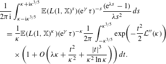 $$\begin{eqnarray}\displaystyle & & \displaystyle \frac{1}{2\unicode[STIX]{x1D70B}\text{i}}\int _{\unicode[STIX]{x1D705}-\text{i}\unicode[STIX]{x1D705}^{3/5}}^{\unicode[STIX]{x1D705}+\text{i}\unicode[STIX]{x1D705}^{3/5}}\mathbb{E}(L(1,\mathbb{X})^{s})(\text{e}^{\unicode[STIX]{x1D6FE}}\unicode[STIX]{x1D70F})^{-s}\frac{(\text{e}^{\unicode[STIX]{x1D706}s}-1)}{\unicode[STIX]{x1D706}s^{2}}\,ds\nonumber\\ \displaystyle & & \displaystyle \quad =\frac{1}{\unicode[STIX]{x1D705}}\mathbb{E}(L(1,\mathbb{X})^{\unicode[STIX]{x1D705}})(\text{e}^{\unicode[STIX]{x1D6FE}}\unicode[STIX]{x1D70F})^{-\unicode[STIX]{x1D705}}\frac{1}{2\unicode[STIX]{x1D70B}}\int _{-\unicode[STIX]{x1D705}^{3/5}}^{\unicode[STIX]{x1D705}^{3/5}}\exp \biggl(-\frac{t^{2}}{2}{\mathcal{L}}^{\prime \prime }(\unicode[STIX]{x1D705})\biggr)\nonumber\\ \displaystyle & & \displaystyle \qquad \times \,\biggl(1+O\biggl(\unicode[STIX]{x1D706}\unicode[STIX]{x1D705}+\frac{t^{2}}{\unicode[STIX]{x1D705}^{2}}+\frac{|t|^{3}}{\unicode[STIX]{x1D705}^{2}\ln \unicode[STIX]{x1D705}}\biggr)\biggr)\,dt.\end{eqnarray}$$
Further, from (4.10) we have
 ${\mathcal{L}}^{\prime \prime }(\unicode[STIX]{x1D705})\asymp 1/(\unicode[STIX]{x1D705}\ln \unicode[STIX]{x1D705})$
, so there exists a positive constant
${\mathcal{L}}^{\prime \prime }(\unicode[STIX]{x1D705})\asymp 1/(\unicode[STIX]{x1D705}\ln \unicode[STIX]{x1D705})$
, so there exists a positive constant
 $b_{4}$
such that
$b_{4}$
such that
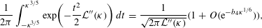 $$\begin{eqnarray}\frac{1}{2\unicode[STIX]{x1D70B}}\int _{-\unicode[STIX]{x1D705}^{3/5}}^{\unicode[STIX]{x1D705}^{3/5}}\exp \biggl(-\frac{t^{2}}{2}{\mathcal{L}}^{\prime \prime }(\unicode[STIX]{x1D705})\biggr)\,dt=\frac{1}{\sqrt{2\unicode[STIX]{x1D70B}{\mathcal{L}}^{\prime \prime }(\unicode[STIX]{x1D705})}}(1+O(\text{e}^{-b_{4}\unicode[STIX]{x1D705}^{1/6}})),\end{eqnarray}$$
and
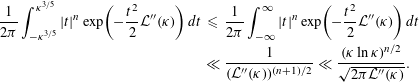 $$\begin{eqnarray}\displaystyle \frac{1}{2\unicode[STIX]{x1D70B}}\int _{-\unicode[STIX]{x1D705}^{3/5}}^{\unicode[STIX]{x1D705}^{3/5}}|t|^{n}\exp \biggl(-\frac{t^{2}}{2}{\mathcal{L}}^{\prime \prime }(\unicode[STIX]{x1D705})\biggr)\,dt & {\leqslant} & \displaystyle \frac{1}{2\unicode[STIX]{x1D70B}}\int _{-\infty }^{\infty }|t|^{n}\exp \biggl(-\frac{t^{2}}{2}{\mathcal{L}}^{\prime \prime }(\unicode[STIX]{x1D705})\biggr)\,dt\nonumber\\ \displaystyle & \ll & \displaystyle \frac{1}{({\mathcal{L}}^{\prime \prime }(\unicode[STIX]{x1D705}))^{(n+1)/2}}\ll \frac{(\unicode[STIX]{x1D705}\ln \unicode[STIX]{x1D705})^{n/2}}{\sqrt{2\unicode[STIX]{x1D70B}{\mathcal{L}}^{\prime \prime }(\unicode[STIX]{x1D705})}}.\nonumber\end{eqnarray}$$
Inserting these estimates into (4.25) we get
 $$\begin{eqnarray}\displaystyle & & \displaystyle \frac{1}{2\unicode[STIX]{x1D70B}\text{i}}\int _{\unicode[STIX]{x1D705}-\text{i}\unicode[STIX]{x1D705}^{3/5}}^{\unicode[STIX]{x1D705}+\text{i}\unicode[STIX]{x1D705}^{3/5}}\mathbb{E}(L(1,\mathbb{X})^{s})(\text{e}^{\unicode[STIX]{x1D6FE}}\unicode[STIX]{x1D70F})^{-s}\frac{(\text{e}^{\unicode[STIX]{x1D706}s}-1)}{\unicode[STIX]{x1D706}s^{2}}\,ds\nonumber\\ \displaystyle & & \displaystyle \quad =\frac{\mathbb{E}(L(1,\mathbb{X})^{\unicode[STIX]{x1D705}})(\text{e}^{\unicode[STIX]{x1D6FE}}\unicode[STIX]{x1D70F})^{-\unicode[STIX]{x1D705}}}{\unicode[STIX]{x1D705}\sqrt{2\unicode[STIX]{x1D70B}{\mathcal{L}}^{\prime \prime }(\unicode[STIX]{x1D705})}}\biggl(1+O\biggl(\unicode[STIX]{x1D706}\unicode[STIX]{x1D705}+\sqrt{\frac{\ln \unicode[STIX]{x1D705}}{\unicode[STIX]{x1D705}}}\biggr)\biggr).\end{eqnarray}$$
Finally, combining the estimates (4.24), (4.26) and choosing
 $\unicode[STIX]{x1D706}=\unicode[STIX]{x1D705}^{-2}$
we obtain the desired result.
$\unicode[STIX]{x1D706}=\unicode[STIX]{x1D705}^{-2}$
we obtain the desired result.
Next we prove (4.5). To do this let
 $0\leqslant \unicode[STIX]{x1D706}\leqslant 1/\unicode[STIX]{x1D705}$
. Using (4.20) from Lemma 4.7, we have
$0\leqslant \unicode[STIX]{x1D706}\leqslant 1/\unicode[STIX]{x1D705}$
. Using (4.20) from Lemma 4.7, we have
 $$\begin{eqnarray}\unicode[STIX]{x1D711}(\text{e}^{-\unicode[STIX]{x1D706}}\unicode[STIX]{x1D70F})-\unicode[STIX]{x1D711}(\unicode[STIX]{x1D70F})\leqslant \frac{1}{2\unicode[STIX]{x1D70B}\text{i}}\int _{\unicode[STIX]{x1D705}-\text{i}\infty }^{\unicode[STIX]{x1D705}+\text{i}\infty }\mathbb{E}(L(1,\mathbb{X})^{s})(\text{e}^{\unicode[STIX]{x1D6FE}}\unicode[STIX]{x1D70F})^{-s}\frac{(\text{e}^{\unicode[STIX]{x1D706}s}-1)}{\unicode[STIX]{x1D706}s}\frac{\text{e}^{\unicode[STIX]{x1D706}s}-\text{e}^{-\unicode[STIX]{x1D706}s}}{s}\,ds.\end{eqnarray}$$
We write
 $s=\unicode[STIX]{x1D705}+\text{i}t$
and split this integral into two pieces:
$s=\unicode[STIX]{x1D705}+\text{i}t$
and split this integral into two pieces:
 $|t|\leqslant \unicode[STIX]{x1D706}\sqrt{\unicode[STIX]{x1D705}\ln \unicode[STIX]{x1D705}}$
and
$|t|\leqslant \unicode[STIX]{x1D706}\sqrt{\unicode[STIX]{x1D705}\ln \unicode[STIX]{x1D705}}$
and
 $|t|>\unicode[STIX]{x1D706}\sqrt{\unicode[STIX]{x1D705}\ln \unicode[STIX]{x1D705}}$
.
$|t|>\unicode[STIX]{x1D706}\sqrt{\unicode[STIX]{x1D705}\ln \unicode[STIX]{x1D705}}$
.
We note that both
 $|(\text{e}^{\unicode[STIX]{x1D706}s}-1)/\unicode[STIX]{x1D706}s|$
and
$|(\text{e}^{\unicode[STIX]{x1D706}s}-1)/\unicode[STIX]{x1D706}s|$
and
 $|(\text{e}^{\unicode[STIX]{x1D706}s}-\text{e}^{-\unicode[STIX]{x1D706}s})/\unicode[STIX]{x1D706}s|$
are less than
$|(\text{e}^{\unicode[STIX]{x1D706}s}-\text{e}^{-\unicode[STIX]{x1D706}s})/\unicode[STIX]{x1D706}s|$
are less than
 $4$
. Therefore, it follows that the first part of the integral contributes
$4$
. Therefore, it follows that the first part of the integral contributes
 $$\begin{eqnarray}\ll \unicode[STIX]{x1D706}\sqrt{\unicode[STIX]{x1D705}\ln \unicode[STIX]{x1D705}}\mathbb{E}(L(1,\mathbb{X})^{\unicode[STIX]{x1D705}})(\text{e}^{\unicode[STIX]{x1D706}}\unicode[STIX]{x1D70F})^{-\unicode[STIX]{x1D705}}.\end{eqnarray}$$
Then, from Lemma 4.6 the second portion contributes
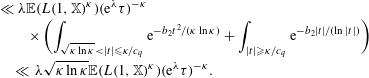 $$\begin{eqnarray}\displaystyle & & \displaystyle \ll \unicode[STIX]{x1D706}\mathbb{E}(L(1,\mathbb{X})^{\unicode[STIX]{x1D705}})(\text{e}^{\unicode[STIX]{x1D706}}\unicode[STIX]{x1D70F})^{-\unicode[STIX]{x1D705}}\nonumber\\ \displaystyle & & \displaystyle \qquad \times \,\biggl(\int _{\sqrt{\unicode[STIX]{x1D705}\ln \unicode[STIX]{x1D705}}<|t|\leqslant \unicode[STIX]{x1D705}/c_{q}}\text{e}^{-b_{2}t^{2}/(\unicode[STIX]{x1D705}\ln \unicode[STIX]{x1D705})}+\int _{|t|\geqslant \unicode[STIX]{x1D705}/c_{q}}\text{e}^{-b_{2}|t|/(\ln |t|)}\biggr)\nonumber\\ \displaystyle & & \displaystyle \quad \ll \,\unicode[STIX]{x1D706}\sqrt{\unicode[STIX]{x1D705}\ln \unicode[STIX]{x1D705}}\mathbb{E}(L(1,\mathbb{X})^{\unicode[STIX]{x1D705}})(\text{e}^{\unicode[STIX]{x1D706}}\unicode[STIX]{x1D70F})^{-\unicode[STIX]{x1D705}}.\nonumber\end{eqnarray}$$
The final result follows from (4.4) and (4.10), specifically they prove:
 $$\begin{eqnarray}\unicode[STIX]{x1D6F7}_{\mathbb{X}}(\unicode[STIX]{x1D70F})\asymp \frac{\mathbb{E}(L(1,\mathbb{X})^{\unicode[STIX]{x1D705}})(\text{e}^{\unicode[STIX]{x1D6FE}}\unicode[STIX]{x1D70F})^{-\unicode[STIX]{x1D705}}}{\unicode[STIX]{x1D705}\sqrt{{\mathcal{L}}^{\prime \prime }(\unicode[STIX]{x1D705})}}\asymp \sqrt{\frac{\ln \unicode[STIX]{x1D705}}{\unicode[STIX]{x1D705}}}\mathbb{E}(L(1,\mathbb{X})^{\unicode[STIX]{x1D705}})(\text{e}^{\unicode[STIX]{x1D6FE}}\unicode[STIX]{x1D70F})^{-\unicode[STIX]{x1D705}}.\end{eqnarray}$$
◻
5 Proofs of Theorem 1.2 and Corollary 1.8
We begin with some notation: let
 $$\begin{eqnarray}\mathbb{P}(L(1,\unicode[STIX]{x1D712}_{D})>\text{e}^{\unicode[STIX]{x1D6FE}}\unicode[STIX]{x1D70F}):=\frac{1}{|{\mathcal{H}}_{n}|}|\{D\in {\mathcal{H}}_{n}:L(1,\unicode[STIX]{x1D712}_{D})>\text{e}^{\unicode[STIX]{x1D6FE}}\unicode[STIX]{x1D70F}\}|\end{eqnarray}$$
and
 $$\begin{eqnarray}M(z):=\frac{1}{|{\mathcal{H}}_{n}|}\mathop{\sum }_{D\in {\mathcal{H}}_{n}}L(1,\unicode[STIX]{x1D712}_{D})^{z}.\end{eqnarray}$$
Proof of Theorem 1.2.
As in § 4.1 let
 $\unicode[STIX]{x1D705}=\unicode[STIX]{x1D705}(\unicode[STIX]{x1D70F})$
be the unique solution to (4.2). Let
$\unicode[STIX]{x1D705}=\unicode[STIX]{x1D705}(\unicode[STIX]{x1D70F})$
be the unique solution to (4.2). Let
 $N$
be a positive integer and
$N$
be a positive integer and
 $0<\unicode[STIX]{x1D706}<\min \{1/(2\unicode[STIX]{x1D705}),1/N\}$
be a real value, which we choose later. Finally, let
$0<\unicode[STIX]{x1D706}<\min \{1/(2\unicode[STIX]{x1D705}),1/N\}$
be a real value, which we choose later. Finally, let
 $Y=b\log |D|/(\log _{2}|D|\log _{3}|D|)$
for some
$Y=b\log |D|/(\log _{2}|D|\log _{3}|D|)$
for some
 $b>0$
small enough.
$b>0$
small enough.
If
 $\log |D|$
is large enough, then for our range of
$\log |D|$
is large enough, then for our range of
 $\unicode[STIX]{x1D70F}$
we have
$\unicode[STIX]{x1D70F}$
we have
 $\unicode[STIX]{x1D705}\leqslant Y$
, which follows from (4.11). Additionally, this means Lemma 3.5 holds for all
$\unicode[STIX]{x1D705}\leqslant Y$
, which follows from (4.11). Additionally, this means Lemma 3.5 holds for all
 $s=\unicode[STIX]{x1D705}+\text{i}t$
as long as
$s=\unicode[STIX]{x1D705}+\text{i}t$
as long as
 $|t|\leqslant Y$
so we consider the following integrals:
$|t|\leqslant Y$
so we consider the following integrals:
 $$\begin{eqnarray}J(\unicode[STIX]{x1D70F})=\frac{1}{2\unicode[STIX]{x1D70B}\text{i}}\int _{\unicode[STIX]{x1D705}-\text{i}\infty }^{\unicode[STIX]{x1D705}+\text{i}\infty }\mathbb{E}(L(1,\mathbb{X})^{s})(\text{e}^{\unicode[STIX]{x1D6FE}}\unicode[STIX]{x1D70F})^{-s}\biggl(\frac{\text{e}^{\unicode[STIX]{x1D706}s}-1}{\unicode[STIX]{x1D706}s}\biggr)^{N}\frac{ds}{s},\end{eqnarray}$$
and
 $$\begin{eqnarray}J_{M}(\unicode[STIX]{x1D70F})=\frac{1}{2\unicode[STIX]{x1D70B}\text{i}}\int _{\unicode[STIX]{x1D705}-\text{i}\infty }^{\unicode[STIX]{x1D705}+\text{i}\infty }M(s)(\text{e}^{\unicode[STIX]{x1D6FE}}\unicode[STIX]{x1D70F})^{-s}\biggl(\frac{\text{e}^{\unicode[STIX]{x1D706}s}-1}{\unicode[STIX]{x1D706}s}\biggr)^{N}\frac{ds}{s}.\end{eqnarray}$$
By Lemma 4.7 we see that
 $$\begin{eqnarray}\unicode[STIX]{x1D6F7}_{\mathbb{X}}(\unicode[STIX]{x1D70F})\leqslant J(\unicode[STIX]{x1D70F})\leqslant \unicode[STIX]{x1D6F7}_{\mathbb{X}}(\text{e}^{-\unicode[STIX]{x1D706}N}\unicode[STIX]{x1D70F})\end{eqnarray}$$
and
 $$\begin{eqnarray}\mathbb{P}(L(1,\unicode[STIX]{x1D712}_{D})>\text{e}^{\unicode[STIX]{x1D6FE}}\unicode[STIX]{x1D70F})\leqslant J_{M}(\unicode[STIX]{x1D70F})\leqslant \mathbb{P}(L(1,\unicode[STIX]{x1D712}_{D})>\text{e}^{\unicode[STIX]{x1D6FE}-\unicode[STIX]{x1D706}N}\unicode[STIX]{x1D70F}).\end{eqnarray}$$
Using that
 $|\text{e}^{\unicode[STIX]{x1D706}s}-1|\leqslant 3$
we have
$|\text{e}^{\unicode[STIX]{x1D706}s}-1|\leqslant 3$
we have
 $$\begin{eqnarray}\displaystyle & & \displaystyle \int _{\unicode[STIX]{x1D705}-\text{i}\infty }^{\unicode[STIX]{x1D705}-\text{i}Y}+\int _{\unicode[STIX]{x1D705}+\text{i}Y}^{\unicode[STIX]{x1D705}+\text{i}\infty }\mathbb{E}(L(1,\mathbb{X})^{s})(\text{e}^{\unicode[STIX]{x1D6FE}}\unicode[STIX]{x1D70F})^{-s}\biggl(\frac{\text{e}^{\unicode[STIX]{x1D706}s}-1}{\unicode[STIX]{x1D706}s}\biggr)^{N}\frac{ds}{s}\nonumber\\ \displaystyle & & \displaystyle \quad \ll \,\frac{1}{N}\biggl(\frac{3}{\unicode[STIX]{x1D706}Y}\biggr)^{N}\mathbb{E}(L(1,\mathbb{X})^{\unicode[STIX]{x1D705}})(\text{e}^{\unicode[STIX]{x1D6FE}}\unicode[STIX]{x1D70F})^{-\unicode[STIX]{x1D705}},\nonumber\end{eqnarray}$$
and similarly, together with Lemma 3.5 we obtain
 $$\begin{eqnarray}\displaystyle & & \displaystyle \int _{\unicode[STIX]{x1D705}-\text{i}\infty }^{\unicode[STIX]{x1D705}-\text{i}Y}+\int _{\unicode[STIX]{x1D705}+\text{i}Y}^{\unicode[STIX]{x1D705}+\text{i}\infty }M(s)(\text{e}^{\unicode[STIX]{x1D6FE}}\unicode[STIX]{x1D70F})^{-s}\biggl(\frac{\text{e}^{\unicode[STIX]{x1D706}s}-1}{\unicode[STIX]{x1D706}s}\biggr)^{N}\frac{ds}{s}\ll \frac{1}{N}\biggl(\frac{3}{\unicode[STIX]{x1D706}Y}\biggr)^{N}M(\unicode[STIX]{x1D705})(\text{e}^{\unicode[STIX]{x1D6FE}}\unicode[STIX]{x1D70F})^{-\unicode[STIX]{x1D705}}\nonumber\\ \displaystyle & & \displaystyle \quad \ll \,\frac{1}{N}\biggl(\frac{3}{\unicode[STIX]{x1D706}Y}\biggr)^{N}\mathbb{E}(L(1,\mathbb{X})^{\unicode[STIX]{x1D705}})(\text{e}^{\unicode[STIX]{x1D6FE}}\unicode[STIX]{x1D70F})^{-\unicode[STIX]{x1D705}}.\nonumber\end{eqnarray}$$
For the remaining parts of the integral we have that
 $|t|\leqslant Y$
so we apply Lemma 3.5, which states that
$|t|\leqslant Y$
so we apply Lemma 3.5, which states that
 $M(s)-\mathbb{E}(L(1,\mathbb{X}))^{s}\ll \mathbb{E}(L(1,\mathbb{X})^{\Re s})/(\log |D|)^{11}$
. Then we use the inequality
$M(s)-\mathbb{E}(L(1,\mathbb{X}))^{s}\ll \mathbb{E}(L(1,\mathbb{X})^{\Re s})/(\log |D|)^{11}$
. Then we use the inequality
 $|(\text{e}^{\unicode[STIX]{x1D706}s}-1)/\unicode[STIX]{x1D706}s|\leqslant 4$
to obtain
$|(\text{e}^{\unicode[STIX]{x1D706}s}-1)/\unicode[STIX]{x1D706}s|\leqslant 4$
to obtain
 $$\begin{eqnarray}J_{M}(\unicode[STIX]{x1D70F})-J(\unicode[STIX]{x1D70F})\ll \frac{1}{N}\biggl(\frac{3}{\unicode[STIX]{x1D706}Y}\biggr)^{N}\mathbb{E}(L(1,\mathbb{X})^{\unicode[STIX]{x1D705}})(\text{e}^{\unicode[STIX]{x1D6FE}}\unicode[STIX]{x1D70F})^{-\unicode[STIX]{x1D705}}+\frac{Y}{\unicode[STIX]{x1D705}}4^{N}\frac{\mathbb{E}(L(1,\mathbb{X})^{\unicode[STIX]{x1D705}})}{(\text{e}^{\unicode[STIX]{x1D6FE}}\unicode[STIX]{x1D70F})^{\unicode[STIX]{x1D705}}(\log |D|)^{11}}.\end{eqnarray}$$
Choosing
 $N=[\log _{2}|D|]$
and
$N=[\log _{2}|D|]$
and
 $\unicode[STIX]{x1D706}=\text{e}^{10}/Y$
then (4.27) gives us that
$\unicode[STIX]{x1D706}=\text{e}^{10}/Y$
then (4.27) gives us that
 $$\begin{eqnarray}J_{M}(\unicode[STIX]{x1D70F})-J(\unicode[STIX]{x1D70F})\ll \frac{\unicode[STIX]{x1D6F7}_{\mathbb{X}}(\unicode[STIX]{x1D70F})}{(\log |D|)^{8}}.\end{eqnarray}$$
On the other hand, by Theorem 1.3 in combination with our choice for
 $\unicode[STIX]{x1D706}$
,
$\unicode[STIX]{x1D706}$
,
 $N$
and
$N$
and
 $Y$
we have
$Y$
we have
 $$\begin{eqnarray}\unicode[STIX]{x1D6F7}_{\mathbb{X}}(\text{e}^{\pm \unicode[STIX]{x1D706}N}\unicode[STIX]{x1D70F})=\unicode[STIX]{x1D6F7}_{\mathbb{ X}}(\unicode[STIX]{x1D70F})\biggl(1+O\biggl(\frac{\text{e}^{\unicode[STIX]{x1D70F}}(\log _{2}|D|)^{2}\log _{3}|D|}{\log |D|}\biggr)\biggr).\end{eqnarray}$$
Hence, combining (5.1), (5.2) and (5.3)
 $$\begin{eqnarray}\displaystyle \mathbb{P}(L(1,\unicode[STIX]{x1D712}_{D})>\text{e}^{\unicode[STIX]{x1D6FE}}\unicode[STIX]{x1D70F}) & {\leqslant} & \displaystyle J_{M}(\unicode[STIX]{x1D70F})\nonumber\\ \displaystyle & {\leqslant} & \displaystyle J(\unicode[STIX]{x1D70F})+O\biggl(\frac{\unicode[STIX]{x1D6F7}_{\mathbb{X}}(\unicode[STIX]{x1D70F})}{(\log |D|)^{8}}\biggr)\nonumber\\ \displaystyle & {\leqslant} & \displaystyle \unicode[STIX]{x1D6F7}_{\mathbb{X}}(\unicode[STIX]{x1D70F})\biggl(1+O\biggl(\frac{\text{e}^{\unicode[STIX]{x1D70F}}\log _{2}|D|\log _{3}|D|}{\log |D|}\biggr)\biggr),\nonumber\end{eqnarray}$$
and
 $$\begin{eqnarray}\displaystyle \mathbb{P}(L(1,\unicode[STIX]{x1D712}_{D})>\text{e}^{\unicode[STIX]{x1D6FE}}\unicode[STIX]{x1D70F}) & {\geqslant} & \displaystyle J_{M}(\text{e}^{\unicode[STIX]{x1D706}N}\unicode[STIX]{x1D70F})\nonumber\\ \displaystyle & {\geqslant} & \displaystyle J(\text{e}^{\unicode[STIX]{x1D706}N}\unicode[STIX]{x1D70F})+O\biggl(\frac{\unicode[STIX]{x1D6F7}_{\mathbb{X}}(\unicode[STIX]{x1D70F})}{(\log |D|)^{8}}\biggr)\nonumber\\ \displaystyle & {\geqslant} & \displaystyle \unicode[STIX]{x1D6F7}_{\mathbb{X}}(\unicode[STIX]{x1D70F})\biggl(1+O\biggl(\frac{\text{e}^{\unicode[STIX]{x1D70F}}(\log _{2}|D|)^{2}\log _{3}|D|}{\log |D|}\biggr)\biggr).\nonumber\end{eqnarray}$$
The final step is done by recalling for
 $D\in {\mathcal{H}}_{n}$
we have
$D\in {\mathcal{H}}_{n}$
we have
 $|D|=q^{n}$
.◻
$|D|=q^{n}$
.◻
And now how to make use of Theorem 1.2 to prove the corollaries of §1.1.
Proof of Corollary 1.8.
We note by Artin’s class number formula given by (1.3) that
 $h_{D}\geqslant \text{e}^{\unicode[STIX]{x1D6FE}}\unicode[STIX]{x1D70F}(\sqrt{|D|}/\sqrt{q})$
if and only if for
$h_{D}\geqslant \text{e}^{\unicode[STIX]{x1D6FE}}\unicode[STIX]{x1D70F}(\sqrt{|D|}/\sqrt{q})$
if and only if for
 $D\in {\mathcal{H}}_{2g+1}$
we have
$D\in {\mathcal{H}}_{2g+1}$
we have
 $L(1,\unicode[STIX]{x1D712}_{D})\geqslant \text{e}^{\unicode[STIX]{x1D6FE}}\unicode[STIX]{x1D70F}$
. Specializing to
$L(1,\unicode[STIX]{x1D712}_{D})\geqslant \text{e}^{\unicode[STIX]{x1D6FE}}\unicode[STIX]{x1D70F}$
. Specializing to
 $n=2g+1$
we see Theorem 1.2 proved that the number of
$n=2g+1$
we see Theorem 1.2 proved that the number of
 $D$
such that
$D$
such that
 $L(1,\unicode[STIX]{x1D712}_{D})>\text{e}^{\unicode[STIX]{x1D6FE}}\unicode[STIX]{x1D70F}$
is given by
$L(1,\unicode[STIX]{x1D712}_{D})>\text{e}^{\unicode[STIX]{x1D6FE}}\unicode[STIX]{x1D70F}$
is given by
 $$\begin{eqnarray}|{\mathcal{H}}_{2g+1}|\unicode[STIX]{x1D6F7}_{\mathbb{X}}(\unicode[STIX]{x1D70F})\biggl(1+O\biggl(\frac{\text{e}^{\unicode[STIX]{x1D70F}}(\log _{2}|D|)^{2}\log _{3}|D|}{\log |D|}\biggr)\biggr).\end{eqnarray}$$
Finally, we use Theorem 1.3 to conclude that the number of
 $D$
such that
$D$
such that
 $h_{D}\geqslant \text{e}^{\unicode[STIX]{x1D6FE}}\unicode[STIX]{x1D70F}(\sqrt{|D|}/\sqrt{q})$
is given by
$h_{D}\geqslant \text{e}^{\unicode[STIX]{x1D6FE}}\unicode[STIX]{x1D70F}(\sqrt{|D|}/\sqrt{q})$
is given by
 $$\begin{eqnarray}\displaystyle & & \displaystyle |{\mathcal{H}}_{2g+1}|\exp \biggl(-C_{1}(q^{\{\log \unicode[STIX]{x1D705}\}})\frac{q^{\unicode[STIX]{x1D70F}-C_{0}(q^{\{\log \unicode[STIX]{x1D705}\}})}}{\unicode[STIX]{x1D70F}}\biggl(1+O\biggl(\frac{\log \unicode[STIX]{x1D70F}}{\unicode[STIX]{x1D70F}}\biggr)\biggr)\biggr)\nonumber\\ \displaystyle & & \displaystyle \qquad \times \,\biggl(1+O\biggl(\frac{\text{e}^{\unicode[STIX]{x1D70F}}(\log _{2}|D|)^{2}\log _{3}|D|}{\log |D|}\biggr)\biggr)\nonumber\\ \displaystyle & & \displaystyle \quad =|{\mathcal{H}}_{2g+1}|\exp \biggl(-C_{1}(q^{\{\log \unicode[STIX]{x1D705}\}})\frac{q^{\unicode[STIX]{x1D70F}-C_{0}(q^{\{\log \unicode[STIX]{x1D705}\}})}}{\unicode[STIX]{x1D70F}}\biggl(1+O\biggl(\frac{\log \unicode[STIX]{x1D70F}}{\unicode[STIX]{x1D70F}}\biggr)\biggr)\biggr),\nonumber\end{eqnarray}$$
where the final estimate follows from the range of
 $\unicode[STIX]{x1D70F}$
. The analogous estimate for small values of
$\unicode[STIX]{x1D70F}$
. The analogous estimate for small values of
 $h_{D}$
follows along the same lines.◻
$h_{D}$
follows along the same lines.◻
6 Optimal
$\unicode[STIX]{x1D6FA}$
-results: proof of Theorem 1.6

For each irreducible polynomial
 $P\in \mathbb{F}_{q}[x]$
, let
$P\in \mathbb{F}_{q}[x]$
, let
 $\unicode[STIX]{x1D6FF}_{P}\in \{-1,1\}.$
Define
$\unicode[STIX]{x1D6FF}_{P}\in \{-1,1\}.$
Define
 ${\mathcal{S}}_{N}(n,\{\unicode[STIX]{x1D6FF}_{P}\})$
to be the set of all monic irreducibles
${\mathcal{S}}_{N}(n,\{\unicode[STIX]{x1D6FF}_{P}\})$
to be the set of all monic irreducibles
 $Q\in \mathbb{F}_{q}[x]$
such that
$Q\in \mathbb{F}_{q}[x]$
such that
 $\deg Q=N$
and
$\deg Q=N$
and
 $$\begin{eqnarray}\biggl(\frac{P}{Q}\biggr)=\unicode[STIX]{x1D6FF}_{P},\end{eqnarray}$$
for all irreducibles
 $P$
with
$P$
with
 $\deg P\leqslant n$
. We also let
$\deg P\leqslant n$
. We also let
 ${\mathcal{P}}(n)$
denote the product of all irreducible polynomials
${\mathcal{P}}(n)$
denote the product of all irreducible polynomials
 $P$
with
$P$
with
 $\deg P\leqslant n$
.
$\deg P\leqslant n$
.
Lemma 6.1. Let
 $N$
be large, and
$N$
be large, and
 $1\leqslant n\leqslant (\log _{q}(N))^{2}$
be a real number. Then, we have
$1\leqslant n\leqslant (\log _{q}(N))^{2}$
be a real number. Then, we have
 $$\begin{eqnarray}|{\mathcal{S}}_{N}(n,\{\unicode[STIX]{x1D6FF}_{P}\})|=\frac{q^{N}}{2^{\unicode[STIX]{x1D6F1}_{q}(n)}N}+O(q^{N/2+n}).\end{eqnarray}$$
Proof. For each monic polynomial
 $f\in \mathbb{F}_{q}[x]$
, define
$f\in \mathbb{F}_{q}[x]$
, define
 $\unicode[STIX]{x1D6FF}_{f}=\prod _{P\mid f}\unicode[STIX]{x1D6FF}_{P}$
. Let
$\unicode[STIX]{x1D6FF}_{f}=\prod _{P\mid f}\unicode[STIX]{x1D6FF}_{P}$
. Let
 $Q$
be an irreducible polynomial of degree
$Q$
be an irreducible polynomial of degree
 $N$
. Then, observe that
$N$
. Then, observe that
 $$\begin{eqnarray}\mathop{\sum }_{f\mid {\mathcal{P}}(n)}\unicode[STIX]{x1D6FF}_{f}\biggl(\frac{f}{Q}\biggr)=\mathop{\prod }_{\deg P\leqslant n}\biggl(1+\unicode[STIX]{x1D6FF}_{P}\biggl(\frac{P}{Q}\biggr)\biggr)=\left\{\begin{array}{@{}ll@{}}2^{\unicode[STIX]{x1D6F1}_{q}(n)}\quad & \text{if }Q\in {\mathcal{S}}_{N}(n,\{\unicode[STIX]{x1D6FF}_{P}\}),\\ 0\quad & \text{otherwise}.\end{array}\right.\end{eqnarray}$$
Therefore, we deduce that
 $$\begin{eqnarray}|{\mathcal{S}}_{N}(n,\{\unicode[STIX]{x1D6FF}_{P}\})|=\frac{1}{2^{\unicode[STIX]{x1D6F1}_{q}(n)}}\mathop{\sum }_{f\mid {\mathcal{P}}(n)}\unicode[STIX]{x1D6FF}_{f}\mathop{\sum }_{\substack{ Q\text{ irreducible } \\ \deg Q=N}}\biggl(\frac{f}{Q}\biggr).\end{eqnarray}$$
Since all the divisors of
 ${\mathcal{P}}(n)$
are square-free, we obtain from (2.5) that for all
${\mathcal{P}}(n)$
are square-free, we obtain from (2.5) that for all
 $f\neq 1$
such that
$f\neq 1$
such that
 $f\mid {\mathcal{P}}(n)$
, we have
$f\mid {\mathcal{P}}(n)$
, we have
 $$\begin{eqnarray}\mathop{\sum }_{\substack{ Q\text{ irreducible } \\ \deg Q=N}}\biggl(\frac{f}{Q}\biggr)\ll \deg (f)q^{N/2}\ll q^{N/2+n},\end{eqnarray}$$
since
 $$\begin{eqnarray}\deg f\leqslant \deg {\mathcal{P}}(n)=\mathop{\sum }_{j=1}^{n}j\unicode[STIX]{x1D70B}_{q}(j)\asymp q^{n},\end{eqnarray}$$
by the prime number theorem. Finally, since the number of divisors of
 ${\mathcal{P}}(n)$
is
${\mathcal{P}}(n)$
is
 $2^{\unicode[STIX]{x1D6F1}_{q}(n)}$
we deduce that
$2^{\unicode[STIX]{x1D6F1}_{q}(n)}$
we deduce that
 $$\begin{eqnarray}|{\mathcal{S}}_{N}(n,\{\unicode[STIX]{x1D6FF}_{P}\})|=\frac{\unicode[STIX]{x1D70B}_{q}(N)}{2^{\unicode[STIX]{x1D6F1}_{q}(n)}}+O(q^{N/2+n}),\end{eqnarray}$$
which completes the proof. ◻
We shall deduce Theorem 1.6 from the following proposition.
Proposition 6.2. We have
 $$\begin{eqnarray}\mathop{\sum }_{Q\in {\mathcal{S}}_{N}(n,\{\unicode[STIX]{x1D6FF}_{P}\})}L(1,\unicode[STIX]{x1D712}_{Q})=\unicode[STIX]{x1D701}_{\mathbb{A}}(2)\frac{\unicode[STIX]{x1D70B}_{q}(N)}{2^{\unicode[STIX]{x1D6F1}_{q}(n)}}\mathop{\prod }_{\deg P\leqslant n}\biggl(1+\frac{\unicode[STIX]{x1D6FF}_{P}}{|P|}\biggr)+O(N^{2}q^{N/2+2n}).\end{eqnarray}$$
Proof. First, it follows from (2.3) that for all
 $m\geqslant N$
we have
$m\geqslant N$
we have
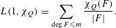 $$\begin{eqnarray}L(1,\unicode[STIX]{x1D712}_{Q})=\mathop{\sum }_{\deg F\leqslant m}\frac{\unicode[STIX]{x1D712}_{Q}(F)}{|F|}.\end{eqnarray}$$
Let
 $A=2N\deg {\mathcal{P}}(n)\ll Nq^{n}$
by (6.2). Then, from (6.1) we obtain
$A=2N\deg {\mathcal{P}}(n)\ll Nq^{n}$
by (6.2). Then, from (6.1) we obtain
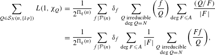 $$\begin{eqnarray}\displaystyle \mathop{\sum }_{Q\in {\mathcal{S}}_{N}(n,\{\unicode[STIX]{x1D6FF}_{P}\})}L(1,\unicode[STIX]{x1D712}_{Q}) & = & \displaystyle \frac{1}{2^{\unicode[STIX]{x1D6F1}_{q}(n)}}\mathop{\sum }_{f\mid {\mathcal{P}}(n)}\unicode[STIX]{x1D6FF}_{f}\mathop{\sum }_{\substack{ Q\text{ irreducible } \\ \deg Q=N}}\biggl(\frac{f}{Q}\biggr)\mathop{\sum }_{\deg F\leqslant A}\frac{(Q/F)}{|F|}\nonumber\\ \displaystyle & = & \displaystyle \frac{1}{2^{\unicode[STIX]{x1D6F1}_{q}(n)}}\mathop{\sum }_{f\mid {\mathcal{P}}(n)}\unicode[STIX]{x1D6FF}_{f}\mathop{\sum }_{\deg F\leqslant A}\frac{1}{|F|}\mathop{\sum }_{\substack{ Q\text{ irreducible } \\ \deg Q=N}}\biggl(\frac{Ff}{Q}\biggr),\nonumber\\ \displaystyle & & \displaystyle\end{eqnarray}$$
by quadratic reciprocity (2.6). Since any divisor
 $f$
of
$f$
of
 ${\mathcal{P}}(n)$
is square-free, it follows that
${\mathcal{P}}(n)$
is square-free, it follows that
 $Ff$
is a square only when
$Ff$
is a square only when
 $F=fh^{2}$
, for some monic polynomial
$F=fh^{2}$
, for some monic polynomial
 $h$
. In this case, we have
$h$
. In this case, we have
 $$\begin{eqnarray}\mathop{\sum }_{\substack{ Q\text{ irreducible } \\ \deg Q=N}}\biggl(\frac{Ff}{Q}\biggr)=\unicode[STIX]{x1D70B}_{q}(N)+O(\unicode[STIX]{x1D714}(F))=\unicode[STIX]{x1D70B}_{q}(N)+O(A),\end{eqnarray}$$
where
 $\unicode[STIX]{x1D714}(F)$
is the number of irreducible divisors of
$\unicode[STIX]{x1D714}(F)$
is the number of irreducible divisors of
 $F$
, and
$F$
, and
 $\unicode[STIX]{x1D714}(F)\leqslant \deg F\leqslant A$
.
$\unicode[STIX]{x1D714}(F)\leqslant \deg F\leqslant A$
.
Furthermore, if
 $Ff$
is not a square, then by (2.5) we get
$Ff$
is not a square, then by (2.5) we get
 $$\begin{eqnarray}\mathop{\sum }_{\substack{ Q\text{ irreducible } \\ \deg Q=N}}\biggl(\frac{Ff}{Q}\biggr)\ll \deg (Ff)q^{N/2}\ll Aq^{N/2},\end{eqnarray}$$
by (6.2). Inserting these estimates in (6.4), we deduce
 $$\begin{eqnarray}\mathop{\sum }_{Q\in {\mathcal{S}}_{N}(n,\{\unicode[STIX]{x1D6FF}_{P}\})}L(1,\unicode[STIX]{x1D712}_{Q})=\frac{\unicode[STIX]{x1D70B}_{q}(N)}{2^{\unicode[STIX]{x1D6F1}_{q}(n)}}\mathop{\sum }_{f\mid {\mathcal{P}}(n)}\frac{\unicode[STIX]{x1D6FF}_{f}}{|f|}\mathop{\sum }_{\deg h\leqslant (A-\deg f)/2}\frac{1}{|h|^{2}}+O(A^{2}q^{N/2}),\end{eqnarray}$$
since
 $$\begin{eqnarray}\mathop{\sum }_{\deg F\leqslant A}\frac{1}{|F|}=\mathop{\sum }_{k=1}^{A}\mathop{\sum }_{\deg F=k}\frac{1}{q^{k}}=A.\end{eqnarray}$$
Finally, since
 $\deg f\leqslant \deg {\mathcal{P}}(n)\leqslant A/2$
, then for all
$\deg f\leqslant \deg {\mathcal{P}}(n)\leqslant A/2$
, then for all
 $f\mid {\mathcal{P}}(n)$
we have that the tail of the inner sum is very small:
$f\mid {\mathcal{P}}(n)$
we have that the tail of the inner sum is very small:
 $$\begin{eqnarray}\mathop{\sum }_{\deg h>(A-\deg f)/2}\frac{1}{|h|^{2}}\leqslant \mathop{\sum }_{\deg h>A/2}\frac{1}{|h|^{2}}\leqslant \mathop{\sum }_{k>A/2}\frac{1}{q^{2k}}\ll q^{-N}.\end{eqnarray}$$
Inserting this estimate in (6.5) completes the proof. ◻
We finish this section by proving Theorem 1.6.
Proof of Theorem 1.6.
We choose
 $n$
such that
$n$
such that
 $$\begin{eqnarray}\frac{N\log N}{10\unicode[STIX]{x1D701}_{\mathbb{A}}(2)q}\leqslant q^{n}<\frac{N\log N}{10\unicode[STIX]{x1D701}_{\mathbb{A}}(2)}.\end{eqnarray}$$
We choose
 $\unicode[STIX]{x1D6FF}_{P}=1$
for all monic irreducibles
$\unicode[STIX]{x1D6FF}_{P}=1$
for all monic irreducibles
 $P$
with
$P$
with
 $\deg P\leqslant n$
. Then, it follows from Lemma 6.1 and Proposition 6.2 that
$\deg P\leqslant n$
. Then, it follows from Lemma 6.1 and Proposition 6.2 that
 $$\begin{eqnarray}\frac{1}{|{\mathcal{S}}_{N}(n,\{\unicode[STIX]{x1D6FF}_{P}\})|}\mathop{\sum }_{Q\in {\mathcal{S}}_{N}(n,\{\unicode[STIX]{x1D6FF}_{P}\})}L(1,\unicode[STIX]{x1D712}_{Q})=\unicode[STIX]{x1D701}_{\mathbb{A}}(2)\mathop{\prod }_{\deg P\leqslant n}\biggl(1+\frac{1}{|P|}\biggr)(1+O(q^{-N/6})).\end{eqnarray}$$
Furthermore, by Lemma 2.3 we have
 $$\begin{eqnarray}\unicode[STIX]{x1D701}_{\mathbb{A}}(2)\mathop{\prod }_{\deg P\leqslant n}\biggl(1+\frac{1}{|P|}\biggr)=\mathop{\prod }_{\deg P\leqslant n}\biggl(1-\frac{1}{|P|}\biggr)^{-1}\biggl(1+O\biggl(\frac{q^{-n}}{n}\biggr)\biggr)=\text{e}^{\unicode[STIX]{x1D6FE}}n+O(1).\end{eqnarray}$$
Combining this estimate with (6.6) and (6.7) yields the existence of a monic irreducible
 $Q$
of degree
$Q$
of degree
 $N$
, such that
$N$
, such that
 $$\begin{eqnarray}L(1,\unicode[STIX]{x1D712}_{Q})\geqslant \text{e}^{\unicode[STIX]{x1D6FE}}\log (N\log N)+O(1)=\text{e}^{\unicode[STIX]{x1D6FE}}(\log _{2}|Q|+\log _{3}|Q|)+O(1),\end{eqnarray}$$
as desired. Finally, one can deduce (1.14) along the same lines by taking
 $\unicode[STIX]{x1D6FF}_{P}=-1$
for all monic irreducibles
$\unicode[STIX]{x1D6FF}_{P}=-1$
for all monic irreducibles
 $P$
with
$P$
with
 $\deg P\leqslant n$
.◻
$\deg P\leqslant n$
.◻


