


NOMENCLATURE
- a
simplified dynamics acceleration
-
 $${\mib{{\hskip 3.5pt \vskip -6pt\tilde}{\hskip -3.5pt A}}}$$
state matrix of the linear discrete dynamics
- b
linear constraint vector
-
$${\mib{{\hskip 3.5pt \vskip -6pt\tilde}{\hskip -3.5pt B}}}$$
input matrix of the linear discrete dynamics
- c
QP problem cost vector
-
${\mib{{\hskip 3.5pt \vskip -6pt\tilde}{\hskip -3.5pt C}}} $
output matrix of the linear discrete dynamics
- C D
drag coefficient
- C L
lift coefficient
- D
drag force
-
${\mib{{\hskip 3.5pt \vskip -6pt\tilde}{\hskip -3.5pt D}}}$
feedthrough matrix of the linear discrete dynamics
- DOF
degree–of–freedom
- e
total specific energy
- EOM
equations of motion
-
$$\dot{e}_{{scan}} $$
total specific energy rate value when in scan mode for latching the climb mode
-
$$\dot{e}_{{src}} $$
total specific energy rate value when in search mode for latching the scan mode
- f
EOM right-hand side vector
- f fr
system free response vector
- f fr ,0
system free response vector–linearisation point offset correction
- g
acceleration due to gravity
- G
control variation influence matrix
- GNSS
Global Navigation Satellite System
- GR
glide ratio
-
$${\scr H}$$
QP problem Hessian matrix
- IMU
inertial measurement unit
- j
sampling step
- J
cost/objective function
- k
prediction step
- L
lift force
-
$${L \over D}$$
lift-to-drag ratio
- m
aircraft mass
- M
number of steps in the control horizon
- MPC
model-based predictive control
- N
number of steps in the prediction horizon
- NLP
non-linear programming
- N te
maximum number of data points used for thermal estimation
- N wpt
maximum number of data points used for waypoint calculation
- Q
base weighting matrix associated to the output deviation
-
$${\cal Q}$$
weighting matrix associated to the output deviation
- QP
quadratic programming
- r
polar co-ordinate
- R
base weighting matrix associated to the input action
-
$${\scr R}$$
weighting matrix associated to the input action
- RoC
rate of climb
- R t,x
thermal reference radius in x direction
- R t,y
thermal reference radius in y direction
- s
MacCready’s speed to fly function
- S
wing area
- S
linear constraint matrix
- t
time
- u
control vector
- UAV
unmanned aerial vehicle
- V
airspeed
- V t,max
thermal maximum intensity
- V t,z
air mass vertical velocity derived from a thermal model
- V t,z
vector of stored V t,z values
- V w,z
air mass vertical velocity
- V w , z
vector of stored V w,z values
- V z
aircraft sink rate
- w
simplified dynamics integration function
- x
Cartesian co-ordinate
- x
state vector
- XY
vector of stored (x,y) coordinate values
- y
Cartesian co-ordinate
- y
output vector
-
$${\mib{{\hskip 3.5pt \vskip -4pt\hat}{\hskip -3.5pt Y}}}$$
output vector history throughout the prediction horizon
- Y r
set-point vector throughout the prediction horizon
-
$${\mib{{\hskip 3.5pt \vskip -4pt\hat}{\hskip -3.5pt Y}}}_{\mib{{traj}}} $$
vector of trajectory history throughout the prediction horizon
- z
Cartesian co-ordinate
-
$$\dot{z}_{{mcrd}} $$
expected climb rate within the next thermal


Greek symbols
- α scan
scan mode time factor for latching the climb mode
-
$${\rm \bibeta }_{\mib{{te}}} $$
vector of decision variables of the thermal estimation problem
- γ
flight path angle
- Γ
stage cost function
- Δh clb
minimum height gain needed to keep climb mode latched
- Δr wpt
waypoint tolerance radius
- ΔT
sampling time for prediction & dynamics discretisation
- ΔT clb
time interval for height gain evaluation in climb mode
- ΔT ref
time interval for reference trajectory update by the high level controller
- ΔT scan
total scan mode operation time
- ΔT src
minimum search mode operation time before latching the scan mode
- ΔT te
sampling time for storing thermal estimation data
- ΔT wpt
sampling time for storing waypoint calculation data
- Δ u
control vector variation
- Δ U
control vector variation throughout the control horizon
- η
thermal orientation angle
- θ
polar co-ordinate
-
$${\rm \bixi }$$
augmented state vector
- φ
bank angle
-
$$\biphi $$
system free response state matrix
-
$$\biphi _{\bf {0}}} $$
system free response state derivative matrix
- ψ
heading angle
- ω
simplified dynamics angular velocity
- Ω
terminal cost function


Subscripts
- cart
Cartesian coordinate system
- f
final
- I
aircraft position in an earth-fixed Cartesian co-ordinate system
- lo
lower bound
- max
maximum
- min
minimum
- pol
polar co-ordinate system
- r
reference (set-point) value
- scan
scan mode
- ss
steady-state
- t
position with respect to the thermal centre
- te
thermal estimation
- up
upper bound
- wpt
waypoint
- 0
initial/origin/linearisation point
Superscripts
- T
transpose
- ~
variation from the linearisation reference point
- ^
predicted value
- '
acquired data
- *
solution of the optimal control problem
1.0 INTRODUCTION
For a long time, the atmospheric energy potential in the form of rising air currents (thermals) has been explored by glider pilots and soaring birds, allowing them to remain aloft for long periods of time, eventually covering considerable distances. However, such availability of “clean” energy still seems to be underestimated outside the sportive and recreational fields. Only recently the subject has started to receive serious attention from the aeronautical engineering community as a way of enhancing the performance of powered fixed-wing aircraft during ordinary missions, resulting, at the same time, in more efficient and environment-friendly operations. A number of studies have been conducted, mainly during the past 12 years, which proposed and even flight tested guidance and control algorithms for autonomous soaring flights. They have focused not only on the thermaling approach but also on the exploration of different atmospheric/geographical phenomena, such as wind gradients and slope lift. The widespread usage of unmanned aerial vehicles (UAV), that are frequently equipped with customisable digital flight control hardware, makes them the most natural candidates to incorporate such autonomous capabilities, providing gains in terms of endurance and range.
Small-scale convective air currents are the most common source of lift used by glider pilots. Having as basic requirement the ground exposition to the solar radiation, thermals occur over different areas, from flatlands to mountains. Obviously their characteristics depend on the atmospheric conditions, insolation level and terrain features. Nevertheless, sufficiently strong updrafts are known to be available throughout all the seasons of the year( 1 ). Given its major importance, only the thermal phenomenon is treated herein.
A typical thermal soaring flight can be split into two different and alternate phases: climbing and searching. The climbing stage occurs when the pilot already knows he is flying close to a usable source of lift and manoeuvres to harvest the maximum amount of energy, normally trying to establish a circular path around the core of the rising air column (“thermal centring”). After the updraft is abandoned (normally because it is vanishing) the searching phase begins, when a new lift zone has to be located in time to avoid outlanding. The sort of actions to be taken during this stage is governed by the mission objective. It is essential that an autonomous soaring controller incorporates specific algorithms for dealing with both flying phases, switching between them when appropriate.
Obviously, locating rising air zones is a key aspect of unpowered flight. Pilots normally rely on instrument readings (e.g. variometre) for taking immediate actions and on visual clues for longer-term navigation, such as clouds, terrain characteristics and soaring birds. A database fed with landscape information and past thermal observations could also be used to enhance the search. However, for working autonomously, most of those recognition methods would require complex hardware to be onboard, like infrared cameras or computers with high storage requirements and image processing capability. An alternative and simpler approach is to use only basic instrument data which is more or less what a human pilot does when gliding at reasonable height in clear blue sky days. Therefore, with the objective of allowing wider and less expensive applications, the guidance and control algorithms presented herein assume the UAV is equipped only with a minimal set of hardware, namely, a Pitot-static system, a Global Navigation Satellite System (GNSS) receiver and an Inertial Measurement Unit (IMU).
Most soaring controllers that have been proposed and tested (both numerically and in flight) are based on classical control schemes (see Section 1.1). Despite the fact that they may be robust, optimisation is generally not a design driver. On the other hand, the thermal flight is actually a constant pursuit of maximum climb rate in an uncertain atmospheric environment. Rising air columns of different shapes and intensities can be found in a single mission and those parametres may rapidly change with respect to time and altitude( 1 ). A better performance could be expected if the guidance and control algorithm had the capability to somehow identify and adapt to those variations in real-time. Another important aspect is that optimal climb rates typically result in the airplane flying close to its operational limitations with large amplitude of commands to manoeuvre accordingly.
The above-listed aspects, inherent to soaring, may impose certain limitations to the application of classical control techniques. Nevertheless, the MPC approach seems to be an adequate tool for dealing with them( Reference Maciejowsky 2 ), since
∙ It relies on an internal dynamic model responsible for predicting the time history of the states under the action of a command sequence. This model can incorporate a proper thermal representation and its parametres can be iteratively changed to describe different atmospheric scenarios.
∙ The commands to be applied at a certain instant of time result from the solution of an optimal control problem which can be written to mathematically express the energy gain goal.
∙ MPC algorithms can naturally incorporate constraints in such a way that they are respected by the controller during the predictions.
As explained in Section 1.2, given the nature of the governing atmospheric phenomena and the kind of manoeuvres typically performed, in principle, for acceptable autonomous soaring performance, a non-linear MPC scheme must be adopted. In fact, full non-linear control algorithms have already been reported and numerical studies demonstrated their feasibility for thermal flight. In this scenario, the main objective of the present work is to describe an alternative MPC approach for solving the autonomous soaring problem. Instead of using the non-linear 3 degree-of-freedom (DOF) equations of motion, the proposed methodology is based on predictions computed with the help of simpler linear models that may receive quasi-steady non-linear corrections only to the extent necessary for capturing the dominant effects. Once converted to discrete time domain, the problem is transcribed to a minimum order non-linear programming (NLP) problem with linear inequalities only, which tends to be simpler to solve, potentially requiring less computational resources.
The paper is divided as follows: Section 1.1 presents some of the most relevant recent works related to the emerging area of autonomous atmospheric energy harvesting by fixed-wing aircraft flying within thermals, while Section 1.2 gives more details on the contributions of the proposed research to the field. Section 2 shows how the soaring goals are mathematically translated to an optimal control problem and how MPC-based methodologies can be implemented to solve it. Furthermore, the main atmospheric and flight dynamics phenomena involved in thermaling are also exposed. A thorough description of the developed algorithms, covering controller design, prediction scheme, NLP solution, thermal estimation, reference trajectories and set-points derivation is given in Section 3. Section 4 covers the simulation framework description and corresponding numerical results. The autonomous soaring controller is tested in a randomly generated thermal scenario with relatively fast time-varying characteristics, demonstrating the feasibility of the methodology. Finally, Section 5 summarises the main conclusions derived from this study.
1.1 Previous works
Allen( Reference Allen 3 ) presented a quantitative study of the performance improvements a small electric-powered UAV with a 2h nominal endurance could obtain using updrafts. Simplified flight simulations fed with a large database of meteorological measurements predicted significant benefits achievable year-round, with endurance increase of up to 6h in winter and 12h in summer. Following those positive perspectives, Allen( Reference Allen 4 ) proposed and successfully flight tested the first practical autonomous soaring system on a 4.27m span motor-glider equipped with a commercial autopilot package modified to include the developed outer-loop codes. Total energy rate and acceleration, derived from measurements, are the basic inputs to the algorithm, which is able to estimate the thermal centre and also to calculate its radius by fitting an assumed axisymmetric vertical velocity profile. A simple procedure for estimating and taking into account the thermal drift due to the wind is included. For thermaling, a reference radius and corresponding steady-state turn rate are defined heuristically. Turn rate commands aiming to drive the position and velocity errors to zero are generated by the algorithm and sent to the inner-loop controller. Additionally, through a simple proportional gain term, those commands are also modified in order to respond to changes in total energy acceleration, emulating a technique typically adopted by glider pilots for centring an updraft.
The work by Allen( Reference Allen 4 ) was extended by a series of studies( Reference Edwards 5 , Reference Edwards and Silverberg 6 , Reference Andersson, Kaminer, Dobrokhodov and Cichella 7 , Reference Daugherty and Langelaan 8 , Reference Edwards 9 , Reference Kahn 10 ) that proposed algorithm updates or the inclusion and validation of new features. Moreover, additional numerical and flight testing was pursued. Some of the aspects covered by those works are the following: vehicle total energy and vertical air mass velocity calculation; estimation of thermal parametres (e.g. centre, radius, strength); filtering and lag treatment of measured signals; improvement of the thermal centring process; horizontal wind speed estimation and treatment of corresponding updraft drift; inter-thermal flight strategies; stability and convergence properties of the thermal centring controller. Robust and reliable designs were obtained, as well illustrated by Edwards and Silverberg( Reference Edwards and Silverberg 6 ), who implemented an autonomous soaring controller on a 5 kg, 4.3m span platform which placed third in a cross-country competition against remotely controlled gliders. Furthermore, autonomous flights with range and endurance on the order of 100 km and 5h respectively have been reported( Reference Edwards 9 ) .
While the previously cited works employed classical control techniques, the studies by Lee et al( Reference Lee, Longo and Kerrigan 11 ) and Liu et al( Reference Liu, Schijndel, Longo and Kerrigan 12 ) investigated the autonomous thermal soaring problem in a more formal way, writing it as an optimal control problem to be solved using a non-linear MPC-based scheme applied to the non-linear 3 DOF equations of motion (the potential advantages of using a MPC approach are previously listed in Section 1). State and control constraints were present and different cost functions were tested for the search mode, while in climb mode, the maximisation of the total specific energy was the goal. For the updraft estimation, no predefined thermal shape was assumed. The methodology was evaluated through several numerical simulations where an unpowered UAV was restricted to fly within a 4 km wide square airspace subjected to a thermal environment with non-homogeneous distributed updraft and downdraft areas. The results indicated that the controller was able to avoid sinking zones, explore the area, identify and exploit thermal cores with overall performance depending on the algorithm parametres and on the search method adopted. Therefore, the conceptual feasibility of a MPC controller for extending the loiter time was demonstrated.
The numerical and flight test results reported in the aforementioned references not only demonstrate the feasibility of autonomous thermal soaring techniques but also indicate they are becoming mature and promising strategies to improve the performance of fixed-wing aircraft. However, except when special weather conditions are found, a UAV could hardly rely on soaring only to accomplish typical missions on a daily basis. Hence, one of the upcoming challenges is to integrate those emerging technologies on current powered aircraft in a straightforward and reliable way. Such a scenario was analysed by Edwards( Reference Edwards 13 ), who studied the application of an autonomous thermal controller on an existing hydrogen fuel-cell powered UAV aiming to increase the vehicle’s endurance when flying a communications relay task with altitude band and area overfly constraints. In a similar effort, Bird and Langelaan( Reference Bird and Langelaan 14 ) explored the usage of convective atmospheric energy by hybrid solar/soaring aircraft to overcome limitations of conventional pure solar designs (e.g. low power density and limited wing loading range) and achieve performance maximisation. Those works suggest that soaring algorithms may progressively become a standard tool to be incorporated into the autonomous flight systems of different airplanes. Certainly, this transition process can be accelerated by the development of alternative methodologies like the one proposed herein.
1.2 Present work contribution
A potential drawback of the methodology introduced by Lee et al( Reference Lee, Longo and Kerrigan 11 ) and Liu et al( Reference Liu, Schijndel, Longo and Kerrigan 12 ) is the relatively high computational costs that could hamper the implementation on flight hardware, since solution times of the order of the sampling interval were reported during workstation simulations. For that reason, possible code optimisations, alternative implementations and faster methods are suggested as future developments( Reference Lee, Longo and Kerrigan 11 ). In addition to that, due to the non-linear prediction scheme adopted, the process of converting the optimisation problem to the NLP format becomes more complex. Bearing that in mind, the present work aims to contribute by proposing a simpler yet practical MPC controller which could potentially lead to faster computations and a more straightforward implementation. Three main aspects make the present methodology innovative:
1. The optimal control problem related to soaring is inherently non-linear because the updraft intensity distribution is itself non-linear (in space and time) and significant variations on the aircraft states usually take place when climb or search manoeuvres are executed. Moreover, the usually long prediction horizons necessary for proper thermal centring tend to aggravate that behaviour. Therefore, under those circumstances, the direct use of a linear model (airplane and thermal) for prediction will lead to poor results with significant discrepancies after few seconds. Knowing that, Lee et al( Reference Lee, Longo and Kerrigan 11 ) and Liu et al( Reference Liu, Schijndel, Longo and Kerrigan 12 ) have used fully non-linear 3 DOF point-mass equations for prediction. In order to implement the NLP solution in this framework, normally the differential constraints have to be translated to algebraic non-linear constraints and consequently more variables (associated to the states) need to be introduced, leading to a larger problem. Furthermore, regular bound constraints become non-linear restrictions too. The proposed work provides a simpler yet functional alternative, preserving the main advantages that a linear MPC scheme offers. Its focus relies on using linear prediction models as much as possible, while applying pertinent corrections to take into account some of the leading phenomena governing soaring flight. A key aspect is that the differential constraints are imposed as straightforward matrix operations, therefore all the restrictions remain linear and the order of the problem is reduced, because only the controls are treated as variables. Besides the potential to faster and more efficient computation, those features facilitate the translation to a smaller and less complex NLP problem, allowing simpler numerical algorithms to be used for its solution. Consequently, easier integration on flight hardware is also expected.
2. Different search mode algorithms have been proposed and tested by Lee et al( Reference Lee, Longo and Kerrigan 11 ) and Liu et al( Reference Liu, Schijndel, Longo and Kerrigan 12 ). Some of them are devoted to make the aircraft perform a systematic scan of the airspace, while others aim to avoid previously visited areas. Although all the strategies yielded satisfactory results during the simulations, a difficulty is the need to deal with a non-linear optimisation problem at each time step (as when the climb mode is active), whose solution, depending on some of the involved parametres, may become too costly( Reference Liu, Schijndel, Longo and Kerrigan 12 ). In order to bypass heavy online calculations, a simpler search method is introduced herein. It works by calculating a target waypoint from a least squares problem solution, aiming to maximise the distance from recently scanned zones and to avoid the airspace boundaries. Once the desired location is reached, a new waypoint is assigned. Moreover, the reference airspeed is constantly derived from MacCready’s speed to fly rule. The approach resembles the PVH method employed by Liu et al( Reference Liu, Schijndel, Longo and Kerrigan 12 ), since it has the combined ability to make the UAV stay away from recently searched areas and accelerate to quickly leave downdrafts. The fundamental advantage is that a fully linear prediction model can be applied for the heading and airspeed tracking, resulting in a simpler quadratic optimisation problem to be solved at each time step. Furthermore, the UAV is allowed to cross previously used flight paths, thus avoiding the risk of ‘getting trapped’ as may occur with the PVH method( Reference Liu, Schijndel, Longo and Kerrigan 12 ).
3. Lee et al( Reference Lee, Longo and Kerrigan 11 ) and Liu et al( Reference Liu, Schijndel, Longo and Kerrigan 12 ) have implemented a global thermal mapping algorithm that keeps a record of measured updraft intensities throughout the entire flying zone and adopts no predefined thermal shape. Instead, a Generalised Regression Neural Network (GRNN) is used for obtaining an estimation of the vertical wind velocity field. That approach allows the aircraft to ignore or abandon a weak thermal, latch the search mode for exploring the surroundings and, if the quest is unsuccessful, return to a previously visited area where the stronger lift was detected. The methodology works perfectly in a static or slow time varying environment where, in principle, areas already scanned need not to be searched again. However, thermal life cycles may be short, on the order of few minutes, their intensity generally depends on the height and they drift in response to strong horizontal winds( 1 ). Therefore, in fast time varying atmospheric scenarios, the usefulness of a global mapping is questionable. In other words, there may be no advantage at all in leaving a current weak but sufficiently strong thermal for searching a relatively distant area expecting to come back if no better thermal is found, since the original updraft may have already vanished. For that reason, the present work proposes an online estimation of the environment to be applied only when the climb mode is active and the aircraft is manoeuvring for centring its flight path around the thermal core. Since there is no need for a generic mapping tool that could accommodate several updraft and downdraft zones in a wide area, a predefined local ellipsoidal model suitable for typical thermal shapes is used. As new data are acquired, the model’s parametres are subsequently tuned to fit updraft intensity measurements. Although estimation fidelity may be lost, there is no need to keep a long record of measurements and shorter prediction horizons may be adopted too, since the controller is not ‘concerned’ with the more distant zones.
2.0 PROBLEM FORMULATION
2.1 Equations of motion
The simulations are based on the rigid body 3 DOF point-mass equations (1). The controls are bank angle (φ) and lift coefficient (C L ), which governs the aircraft lift (L), while V is the velocity of the vehicle with respect to the air and V w,z is the air mass vertical velocity representing the environmental effects. No horizontal wind effects were taken into account:
 $$\matrix{ {} \hfill & {\dot{V}{\equals}{1 \over m}\left( {V\left( {m{\rm sin}({\rm \psi }){{\partial V_{{w,z}} } \over {\partial y}}{\rm cos}({\rm \gamma }){\rm sin}({\rm \gamma }){\plus}m{\rm cos}({\rm \psi }){{\partial V_{{w,z}} } \over {\partial x}}{\rm cos}({\rm \gamma }){\rm sin}({\rm \gamma })} \right){\minus}mg{\rm sin}({\rm \gamma }){\minus}D} \right)} \hfill \cr {} \hfill & {{\dot{\rm \gamma }}{\equals}{1 \over {mV}}\left( {V\left( {m{\rm sin}({\rm \psi }){{\partial V_{{w,z}} } \over {\partial y}}{\rm cos}({\rm \gamma })^{2} {\plus}m{\rm cos}({\rm \psi }){{\partial V_{{w,z}} } \over {\partial x}}{\rm cos}({\rm \gamma })^{2} } \right){\minus}mg{\rm cos}({\rm \gamma }){\plus}{\rm cos}(\phi )L} \right)} \hfill \cr {} \hfill & {{\dot{\rm \psi }}{\equals}{{L{\rm sin}(\phi )} \over {\left( {mV{\rm cos}({\rm \gamma })} \right)}}} \hfill \cr {} \hfill & {\dot{x}_{I} {\equals}V{\rm cos}({\rm \gamma }){\rm cos}({\rm \psi })} \hfill \cr {} \hfill & {\dot{y}_{I} {\equals}V{\rm cos}({\rm \gamma }){\rm sin}({\rm \psi })} \hfill \cr {} \hfill & {\dot{z}_{I} {\equals}V_{{w,z}} {\minus}V{\rm sin}({\rm \gamma })} \hfill \cr {} \hfill & {} \hfill \cr } $$
In summarised form, the equations of motion (EOM) can be written as Equation (2), being u the control vector and x cart the state vector, with vehicle’s kinematics written in Cartesian coordinates:
 $$\eqalignno{ & {\bf x}_{{cart}} {\equals}\left[ {\matrix{ V & {\rm \gamma } & {\rm \psi } & {x_{I} } & {y_{I} } & {z_{I} } \cr } } \right]^{T} \cr & {\bf u}{\equals}\left[ {\matrix{ {C_{L} } & \phi \cr } } \right]^{T} \cr & {\dot{\bf x}}_{{cart}} {\equals}{\bf f}_{{cart}} \left( {{\bf x}_{{cart}} ,{\bf u}} \right) $$
When the climb or scan modes are latched a polar co-ordinate system is more appropriate for describing the aircraft motion. The x I and y I state variables are then replaced by r and θ (Equation (3)) with corresponding kinematic equations of motion given by Equation (4):
 $$\eqalignno{ & {\bf x}_{{pol}} {\equals}\left[ {\matrix{ V & {\rm \gamma } & {\rm \psi } & r & {\rm \theta } & {z_{I} } \cr } } \right]^{T} \cr & {\bf u}{\equals}\left[ {\matrix{ {C_{L} } & \phi \cr } } \right]^{T} \cr & {\dot{\bf x}}_{{pol}} {\equals}{\bf f}_{{pol}} \left( {{\bf x}_{{pol}} ,{\bf u}} \right) $$
 $$\eqalignno{ & \dot{r}{\equals}{V \over 2}{\rm sin}({\rm \gamma }{\plus}{\rm \theta }{\minus}{\rm \psi }){\minus}{V \over 2}{\rm cos}({\rm \gamma }{\minus}{\rm \theta }{\plus}{\rm \psi }) \cr & {\dot{\rm \theta }}{\equals}{V \over {2r}}{\rm sin}({\rm \gamma }{\minus}{\rm \theta }{\plus}{\rm \psi }){\minus}{V \over {2r}}{\rm cos}({\rm \gamma }{\plus}{\rm \theta }{\minus}{\rm \psi }) $$
Aircraft performance during soaring flight is essentially governed by its mass and drag polar. The latter is originally available as a selection of discrete (C L ,C D ) pairs and a spline function with an adjustable scalar tension factor is then used to derive the drag coefficient corresponding to any given lift coefficient value, i.e. C D =C D (C L ). This is accomplished with the help of the curv1dp and curv2dp subroutines from Fortran-based Fitgrid interpolation package.Footnote *1 Aerodynamical, geometrical and inertial characteristics of a typical manned 15m span club class glider (summarised in Table 1) are employed in the simulations.
Table 1 Parametres of the aircraft model

a At 81 km/h.
b At 71 km/h.
2.2 Atmospheric effects
The aircraft is subjected to the vertical motion of the air mass, whose velocity V w,z is assumed to be a scalar field function of the Cartesian co-ordinates and time (Equation (5)). In principle, this field does not have restrictions on shape or intensity and may represent any arbitrary atmospheric condition. It is well known that updrafts’ strength and size may vary considerably with the height( Reference Allen 3 ). However, this is not considered in the present work, since the objective is to focus on the challenges imposed by the non-homogeneous shape and time-varying characteristics of the thermal fields.
 $$V_{{w,z}} {\equals}V_{{w,z}} \left( {x_{I} ,y_{I} ,t} \right)$$
Giving the controller the ability to take into account atmospheric perturbations requires the inclusion of a vertical wind mathematical model in the prediction scheme. Different thermal representations can be found in the literature( Reference Thomas 15 ) and, for the present study, a modified model based on the one proposed by Gedeon( Reference Gedeon 16 ) is adopted. It was selected for reflecting two fundamental characteristics which are believed to adequately represent the reality: the intensity decaying as a function of the square of the distance from the core and the consideration of a downdraft zone surrounding the thermal. However, Gedeon’s model( Reference Gedeon 16 ) is axisymmetric, limiting the wind fields it can represent. For this reason, an adjustment is made: two different reference radii are introduced, one for each Cartesian axis, R t,x and R t,y . By doing so the thermal can assume an elliptical format with maximum intensity V t,max, according to Equation (6). Once the basic parametres (R t,x , R t,y and V t,max) are chosen, the estimated updraft vertical speed (V t,z ) at any location (x I ,y I ) can be obtained. Note that the thermal centre position is given by (x t,0,y t,0) and that a rotation angle (η) is also defined. Those terms are adjustable parametres too.
 $$\matrix{ {} \hfill & {V_{{t,z}} {\equals}V_{{t,{\rm max}}} e^{{{\minus}\left[ {\left( {{{x_{t} } \over {R_{{t,x}} }}} \right)^{2} {\plus}\left( {{{y_{t} } \over {R_{{t,y}} }}} \right)^{2} } \right]}} \left[ {1{\minus}\left( {{{x_{t} } \over {R_{{t,x}} }}} \right)^{2} {\minus}\left( {{{y_{t} } \over {R_{{t,y}} }}} \right)^{2} } \right]} \hfill \cr {} \hfill & {x_{t} {\equals}\left( {x_{I} {\minus}x_{{t,0}} } \right){\rm cos}({\rm \eta }){\plus}\left( {y_{I} {\minus}y_{{t,0}} } \right){\rm sin}({\rm \eta })} \hfill \cr {} \hfill & {y_{t} {\equals}{\minus}\left( {x_{I} {\minus}x_{{t,0}} } \right){\rm sin}({\rm \eta }){\plus}\left( {y_{I} {\minus}y_{{t,0}} } \right){\rm cos}({\rm \eta })} \hfill \cr {} \hfill & {} \hfill \cr } $$
2.3 Steady Thermal Flight Optimisation
If one considers a perfectly axisymmetric updraft (e.g., making R
t,x
=R
t,y
in Equation (6)) and a steady atmosphere, then it is possible for a sailplane to remain in an equilibrium condition with constant velocity (V
ss
) and bank angle (φ
ss
), circling at a certain turn rate (
 $$\dot{\psi }_{{ss}} $$
) and radius (r
ss
) relative to the thermal core. Given a specified turn rate and velocity, the permanent flight conditions can be substituted in Equation (1), yielding
$$\dot{\psi }_{{ss}} $$
) and radius (r
ss
) relative to the thermal core. Given a specified turn rate and velocity, the permanent flight conditions can be substituted in Equation (1), yielding
 $$\left\{ {\matrix{ {} \hfill & {\dot{V}{\equals}0} \hfill \cr {} \hfill & {{\dot{\rm \gamma }}{\equals}0} \hfill \cr {} \hfill & {{\dot{\rm \psi }}_{{ss}} {\equals}{{L{\rm sin}(\phi _{{ss}} )} \over {\left( {mV_{{ss}} {\rm cos}({\rm \gamma }_{{ss}} )} \right)}}} \hfill \cr {} \hfill & {\left| {{\dot{\rm \psi }}_{{ss}} r_{{ss}} } \right|{\minus}\left| {V_{{ss}} {\rm cos}({\rm \gamma }_{{ss}} )} \right|{\equals}0} \hfill \cr {} \hfill & {} \hfill \cr } } \right.$$
which is numerically solved for C L,ss , φ ss , r ss and γ ss using Scilab fsolve subroutine. The resulting aircraft sink rate (in calm atmosphere) is then computed as
 $$V_{{ss,z}} {\equals}V_{{ss}} {\rm sin}({\rm \gamma }_{{ss}} )$$
Since the UAV is supposed to be within a thermal, the updraft velocity (function of the radius r ss ) must be added, yielding the final climb/sink rate:
 $${\dot z}_{{I,ss}} {\equals}V_{{ss,z}} {\plus}V_{{t,z}} (r_{{ss}} )$$
Here, two important aspects have to be emphasised( Reference Thomas 15 ): (1) the tighter the curve, the greater the sink rate, V ss,z (for a constant airspeed); (2) the closer to the thermal core the aircraft circles, the greater the vertical wind velocity it encounters. Those two opposed effects represent the essence of thermal flight and are intuitively known by glider pilots. Mathematically, the situation can be described as a static optimisation problem, i.e. for a certain aircraft and updraft shape, it is necessary to find the combination of velocity and turn rate which maximises the climb rate.
As detailed in Section 3.1.1, the above-described behaviour plays a major role in the proposed autonomous soaring algorithm and, in order to consider it, a database is computed offline. Initially, the permanent flight equations (7) are solved for a rectangular grid of (V
ss
,
 $${\dot{\rm \psi }}_{{ss}} $$
) pairs, yielding corresponding V
ss,z
values. Those discrete data feed a bi–spline surface interpolation function with an adjustable scalar tension factor, allowing the sink rate to be obtained for any arbitrary airspeed and turn rate combination. Again, dedicated Fitgrid package subroutines are employed for the numerical implementation, namely surf1dp and surf2dp. Thus, the aircraft vertical velocity in calm atmosphere can be expressed as a function (with the spline based regression procedures embedded) of airspeed and turn rate as indicated by Equation (10).
$${\dot{\rm \psi }}_{{ss}} $$
) pairs, yielding corresponding V
ss,z
values. Those discrete data feed a bi–spline surface interpolation function with an adjustable scalar tension factor, allowing the sink rate to be obtained for any arbitrary airspeed and turn rate combination. Again, dedicated Fitgrid package subroutines are employed for the numerical implementation, namely surf1dp and surf2dp. Thus, the aircraft vertical velocity in calm atmosphere can be expressed as a function (with the spline based regression procedures embedded) of airspeed and turn rate as indicated by Equation (10).
 $$V_{{ss,z}} {\equals}V_{{ss,z}} \left( {V_{{ss}} ,\dot{\psi }_{{ss}} } \right)$$
2.4 Optimal Control Problem
Soaring flight is essentially an optimisation process where the decisions to be taken by the pilot or controller at each instant of time aim to maximise a performance index, normally associated to energy gain or saving. This situation is transcribed to the following optimal control problem:
 $$\matrix{ {} \hfill & {\mathop {\min }\limits_{{\bf u}(t)} J{\equals}\Omega \left( {{\bf x}(t_{f} )} \right){\plus}{\int}_{t_{0} }^{t_{f} } \Gamma \left( {{\bf x}(t),{\bf u}(t),t} \right){\rm d}t} \hfill \cr {{\rm s}{\rm .t}{\rm .}} \hfill & {} \hfill \cr {} \hfill & {{\dot{\bf x}}(t){\equals}{\bf f}\left( {{\bf x}(t),{\bf u}(t),t} \right),\quad t\in\left[ {t_{0} ,t_{f} } \right],} \hfill \cr {} \hfill & {{\bf u}_{{lo}} \leq {\bf u}(t)\leq {\bf u}_{{up}} ,\quad t\in\left[ {t_{0} ,t_{f} } \right],} \hfill \cr {} \hfill & {{\bf x}_{{lo}} \leq {\bf x}(t)\leq {\bf x}_{{up}} ,\quad t\in\left[ {t_{0} ,t_{f} } \right],} \hfill \cr {} \hfill & {} \hfill \cr } $$
whose interpretation is: suppose the aircraft at a given instant of time t
0 and corresponding state
x
(t
0). The objective is to obtain the control and state trajectories (
u
(t),
x
(t)), from t
0 to a fixed t
f
, that minimise the performance index J and, at the same time, respect differential restrictions
 $$\left( {{{\dot{\mib x}}} \left( t \right){\equals}{\mib {f}} \left(\bf{x} } \left( t \right),{\bf{u}} \left( t \right),t} \right)} \right)$$
and lower and upper bounds (
u
lo
,
x
lo
,
u
up
,
x
up
).
$$\left( {{{\dot{\mib x}}} \left( t \right){\equals}{\mib {f}} \left(\bf{x} } \left( t \right),{\bf{u}} \left( t \right),t} \right)} \right)$$
and lower and upper bounds (
u
lo
,
x
lo
,
u
up
,
x
up
).
The differential restrictions are the equations of motion (1), while the control and state bounds represent the aircraft inherent physical limitations (e.g. stall speed), control system restrictions (e.g. actuator saturation) or mission related constraints (e.g. geo-fencing). A certain freedom is allowed in the selection of the performance index, composed by terminal (Ω) and stage (Γ) cost terms. They can be considerably different depending on the active flight mode and their choice is essential for defining the controller behaviour.
2.5 MPC-based solutions
A typical approach for solving Equation (11) involves the discretisation of the state and control trajectories along time so that they are parametrised by a certain number of scalar coefficients. For example, one can split the time interval into small steps (ΔT) and assume that x (t) and u (t) are constant within each time step. Another possibility is to use a functional (e.g. polynomial) basis to approximate the trajectories. In the first case, the state and control values at specific ‘nodes’ themselves are the scalar parametres, while in the second scenario, this role is played by the functions’ coefficients. Once the discretisation is performed, it is possible to rewrite the continuous time problem (Equation (11)) as a NLP problem to be solved for a set of scalar variables. During that process, the differential and bound constraints must be translated accordingly. Many algorithms and softwares which are suitable to numerically solve NLP problems (with different performance levels) are available.Footnote †
The described solution process is a fundamental element of the MPC scheme. At a certain instant of time (t 0), the current state vector ( x (t 0)) is estimated from sensor readings and the discretised version of the optimisation problem (Equation (11)) is numerically solved within a predefined prediction horizon length (t f −t 0). The obtained controls ( u (t)) are then applied to the vehicle during a sampling time interval (ΔT) while the entire calculation process is repeated, so that at the next instant of time (t=t 0+ΔT), a new optimal control sequence is available. This procedure is successively repeated, always with a constant prediction horizon length, which is coherent with the receding horizon strategy.
3.0 ALGORITHM DESCRIPTION
The proposed algorithm operates in three different modes, namely, climb, search and scan, as detailed in Sections 3.1, 3.2 and 3.3, respectively. Section 3.4, on the other hand, describes the overall logic of operation and mode switching rationale.
3.1 Climb mode
When the climb mode is engaged, the controller works in two levels. Initially, a higher level strategy is responsible for generating the reference trajectory and airspeed signals using a simplified dynamics for prediction, whose objective is to maximise the energy gain over the prediction horizon. At this stage, the thermal estimation procedure is also carried out. The produced set-points are then sent to the lower level controller that performs predictions based on a linearised version of the 3 DOF equations of motion. Its goal is to assure that the specified optimal trajectory is tracked accordingly.
3.1.1 High-level controller
Simplified dynamics
We suppose the aircraft dynamics can be transcribed to the following set of equations:
 $$\matrix{ {} \hfill & {\dot{V}{\equals}a} \hfill \cr {} \hfill & {{\dot{\rm \psi }}{\equals}{\rm \omega }} \hfill \cr {} \hfill & {\dot{x}_{I} {\equals}V{\rm cos}({\rm \psi })} \hfill \cr {} \hfill & {\dot{y}_{I} {\equals}V{\rm sin}({\rm \psi })} \hfill \cr {} \hfill & {\dot{z}_{I} {\equals}V_{{t,z}} (x_{I} ,y_{I} ){\plus}V_{{ss,z}} (V,{\rm \omega })} \hfill \cr } $$
They result from Equation (1) after a few simplifications are imposed. One assumes that the effect of the atmospheric perturbation terms
 $${{\partial V_{{w,z}} } \over {\partial x}}$$
and
$${{\partial V_{{w,z}} } \over {\partial x}}$$
and
 $${{\partial V_{{w,z}} } \over {\partial y}}$$
is small and can be ignored. The dynamics of the path angle (
$${{\partial V_{{w,z}} } \over {\partial y}}$$
is small and can be ignored. The dynamics of the path angle (
 $${\dot{\rm \gamma }}$$
) is also neglected and its contribution is assumed to be indirectly contained within a and ω variations. Those two variables, acceleration (a) and angular velocity (ω), are treated as controls, which are actually supposed to be imposed through specific φ and C
L
changes. Moreover, the path angle is assumed to remain small and, therefore, the airspeed (V) and its in-plane component (Vcos(γ)) are presumed to be indistinguishable. V
t,z
, on the other hand, is the updraft velocity estimation given by the elliptical thermal model (Equation (6)), while V
ss,z
is the aircraft sink rate in calm atmosphere and permanent flight condition (Equation (10)).
$${\dot{\rm \gamma }}$$
) is also neglected and its contribution is assumed to be indirectly contained within a and ω variations. Those two variables, acceleration (a) and angular velocity (ω), are treated as controls, which are actually supposed to be imposed through specific φ and C
L
changes. Moreover, the path angle is assumed to remain small and, therefore, the airspeed (V) and its in-plane component (Vcos(γ)) are presumed to be indistinguishable. V
t,z
, on the other hand, is the updraft velocity estimation given by the elliptical thermal model (Equation (6)), while V
ss,z
is the aircraft sink rate in calm atmosphere and permanent flight condition (Equation (10)).
In fact, the system of equations (12) describes the kinematics of the airplane motion to which a quasi-steady correction is applied in order to incorporate the essential effects governing thermal flight (see Section 2.3), i.e. the sink rate versus curve radius relationship and the contribution of the air mass vertical velocity. The fidelity between the two sets of equations (simplified and 3 DOF point-mass) is assured by proper selection of control (a and ω) and control rate (
 $$\dot{a}$$
and
$$\dot{a}$$
and
 $${\dot{\rm \omega }}$$
) bound constraints.
$${\dot{\rm \omega }}$$
) bound constraints.
Cost function
The performance index (Equation (13)), composed by the terminal cost contribution only, is analogous to the one adopted by Lee et al( Reference Lee, Longo and Kerrigan 11 ) and Liu et al( Reference Liu, Schijndel, Longo and Kerrigan 12 ). It denotes the objective of reaching the maximum energy state (kinetic plus potential) at the end of the prediction horizon and is written in terms of the total specific energy. The minus signal is included because in reality a minimisation problem is numerically solved
 $$J{\equals}\Omega \left( {{\bf x}(t_{f} )} \right){\equals}{\minus}\left( {{{V^{2} (t_{f} )} \over {2g}}{\minus}z_{I} (t_{f} )} \right)$$
Prediction
First, the sampling time ΔT and the number of prediction steps N are selected, yielding the prediction horizon NΔT. The control values
 $$({{\hat{\mib u}{\equals}}} \left[ {{\hat{\rm a }}\;{\hat{\rm \omega }}} \right]^{T} )$$
are allowed to change only at each sample time interval and during the first M steps, hence, the control horizon is MΔT. Throughout the remaining steps (up to N)
u
remains constant. The predictions are initially performed using only the first two (linear) equations of the system (12), being
$$({{\hat{\mib u}{\equals}}} \left[ {{\hat{\rm a }}\;{\hat{\rm \omega }}} \right]^{T} )$$
are allowed to change only at each sample time interval and during the first M steps, hence, the control horizon is MΔT. Throughout the remaining steps (up to N)
u
remains constant. The predictions are initially performed using only the first two (linear) equations of the system (12), being
 $$\hat{\mib x}{\equals}\left[ {\hat{V}\;{\hat{\rm \psi }}} \;\right]^T$$
the predicted state vector. Following the translation to discrete time domain, using a zero-order-hold scheme(
Reference Maciejowsky
2
), the system of linear discrete state equations (14) can be obtained:
$$\hat{\mib x}{\equals}\left[ {\hat{V}\;{\hat{\rm \psi }}} \;\right]^T$$
the predicted state vector. Following the translation to discrete time domain, using a zero-order-hold scheme(
Reference Maciejowsky
2
), the system of linear discrete state equations (14) can be obtained:
 $$\eqalignno{ & {\tilde{\rm \bixi }}(k{\plus}1){\equals}{\dot{\rm \bixi }}_{0} \Delta T{\plus}{\tilde{\bf A}}{\rm \bixi }(k){\plus}{\tilde{\bf B}}\Delta {\tilde{\bf u}}(k) \cr & {\tilde{\bf y}}(k{\plus}1){\equals}{\tilde{\bf C}}{\tilde{\rm \bixi }}(k{\plus}1){\plus}{\tilde{\bf D}}\Delta {\tilde{\bf u}}(k{\plus}1) \cr & \Delta {\tilde{\bf u}}(k{\plus}1){\equals}{\tilde{\bf u}}(k{\plus}1){\minus}{\tilde{\bf u}}(k) \cr & {\tilde{\rm \bixi }}(k){\equals}\left\Big[{ {{\tilde{\bf x}}(k)^{T} } & {{\tilde{\bf u}}(k{\minus}1)^{T} } \cr {} & {} \cr } } \right\Big]^{T} $$
They provide the state and output predictions at the step (k+1) from the state and control values at the previous step (k). Note that control variations (
 $$\Delta {{\tilde{\mib u}}} $$
) are used as decision variables, so that an augmented state
$$\Delta {{\tilde{\mib u}}} $$
) are used as decision variables, so that an augmented state
 $${\tilde{\rm \bixi }}$$
has to be employed in order to integrate them, keeping a record of the control amplitudes. Furthermore, the (~) notation indicates variation from the linearisation point (
x
0,
u
0) and, in the current case, the output vector is identical to the state vector, i.e.
$${\tilde{\rm \bixi }}$$
has to be employed in order to integrate them, keeping a record of the control amplitudes. Furthermore, the (~) notation indicates variation from the linearisation point (
x
0,
u
0) and, in the current case, the output vector is identical to the state vector, i.e.
 $${{\tilde{\mib y}}} {\equals}{{\tilde{\mib x}}} {\equals}\tilde[{V}\;{\tilde{\rm \psi }}]^{T} $$
.
$${{\tilde{\mib y}}} {\equals}{{\tilde{\mib x}}} {\equals}\tilde[{V}\;{\tilde{\rm \psi }}]^{T} $$
.
The consecutive application of Equation (14) throughout a prediction horizon of N steps enables one to evaluate the effect of a sequence of control actions
 $$(\Delta {{\hat{\mib U}}} )$$
on the output predicted history
$$(\Delta {{\hat{\mib U}}} )$$
on the output predicted history
 $$\left( {{{\hat{ \mib Y}}} } \right)$$
. By doing so, the system of equations (15) results, where the matrices
$$\left( {{{\hat{ \mib Y}}} } \right)$$
. By doing so, the system of equations (15) results, where the matrices
 $${\bf \Phi } $$
,
$${\bf \Phi } $$
,
 $${\bf \Phi } _{0} $$
and
G
are composed of real and constant elements, while
f
fr
is the system free response vector and
f
fr
,0
stands for the linearisation point offset correction:
$${\bf \Phi } _{0} $$
and
G
are composed of real and constant elements, while
f
fr
is the system free response vector and
f
fr
,0
stands for the linearisation point offset correction:
 $$\eqalignno{ & {\hat{\bf Y}{\equals} {\mib G}}{\bf \Delta } {\hat{\bf U}}{\plus}{\bf f}_{{{\bf fr}}} \cr & {\bf f}_{{{\bf fr}}} {\equals}{\bf \Phi } {\tilde{\rm \bixi }}(k){\plus}{\bf \Phi } _{{\bf 0}} {\rm \bixi }_{0} {\plus}{\bf f}_{{{\bf fr,0}}} \cr & {\hat{\bf Y}}{\equals}[\matrix{ {{\hat{\bf y}}(k{\plus}1\,\mid\,k)^{T} } & {{\hat{\bf y}}(k{\plus}2\,\mid\,k)^{T} } & \,\ldots\, & {{\hat{\bf y}}(k{\plus}N\,\mid\,k)^{T} } \cr } ]^{T} \cr & {\bf \Delta } {\hat{\bf U}}{\equals}[\matrix{ {\Delta {\hat{\bf u}}(k\,\mid\,k)^{T} } & {\Delta {\hat{\bf u}}(k{\plus}1\,\mid\,k)^{T} } & \,\ldots\, & {\Delta {\hat{\bf u}}(k{\plus}M{\minus}1\,\mid\,k)^{T} } \cr } ]^{T} $$
Equations (15) reveal that, as long as the system’s dynamics is linear, the predictions of airspeed and heading angle (contained in vector
 $${{\hat{\mib Y}}} $$
) are obtained by means of straightforward matrix operations. Thereafter, once
$${{\hat{\mib Y}}} $$
) are obtained by means of straightforward matrix operations. Thereafter, once
 $${{\hat{\mib Y}}} $$
and
$${{\hat{\mib Y}}} $$
and
 $$\Delta \hat{\mib U}$$
are known, the last three equations of the system (12) can be integrated via a trapezoidal rule, leading to the aircraft position at each prediction step:
$$\Delta \hat{\mib U}$$
are known, the last three equations of the system (12) can be integrated via a trapezoidal rule, leading to the aircraft position at each prediction step:
 $${\hat{\bf Y}}_{{{\bf traj}}} {\equals}[\matrix{ {\hat{x}_{I} (k{\plus}1\,\mid\,k)} & {\hat{y}_{I} (k{\plus}1\,\mid\,k)} & {\hat{z}_{I} (k{\plus}1\,\mid\,k)} & \,\ldots\, & {\hat{y}_{I} (k{\plus}N\,\mid\,k)} & {\hat{z}_{I} (k{\plus}N\,\mid\,k)} } ]^{T} $$
Two important aspects must be pointed out: (1) given a sequence of control actions, represented by vector
 $$\Delta \hat{\mib U}$$
, the entire predicted output history is obtained explicitly, via simple mathematical operations and, in particular, no implicit integral scheme is necessary; (2) bounds are imposed in the following variables only: airspeed, acceleration, angular speed, acceleration rate and angular speed rate. The system of equations (15) assures that all those constraints remain linear in the entire prediction horizon, hence, they can be put together and written as indicated in Equation (17), where
S
and
b
are a constant real matrix and vector respectively. No bounds are applied to the aircraft position states (x
I
,y
I
,z
I
), because that would need non-linear restrictions to be employed. However, this is not considered critical, since the most important constraints are by far the ones related to the airspeed and controls, given that they reflect actual vehicle performance limitations. Nevertheless, alternative procedures for dealing with airspace boundaries are implemented (see Section 3.2.1):
$$\Delta \hat{\mib U}$$
, the entire predicted output history is obtained explicitly, via simple mathematical operations and, in particular, no implicit integral scheme is necessary; (2) bounds are imposed in the following variables only: airspeed, acceleration, angular speed, acceleration rate and angular speed rate. The system of equations (15) assures that all those constraints remain linear in the entire prediction horizon, hence, they can be put together and written as indicated in Equation (17), where
S
and
b
are a constant real matrix and vector respectively. No bounds are applied to the aircraft position states (x
I
,y
I
,z
I
), because that would need non-linear restrictions to be employed. However, this is not considered critical, since the most important constraints are by far the ones related to the airspeed and controls, given that they reflect actual vehicle performance limitations. Nevertheless, alternative procedures for dealing with airspace boundaries are implemented (see Section 3.2.1):
 $${\bf S}\Delta {\hat{\bf U}}\leq {\bf b}$$
Regarding the cost function (Equation (13)), one can readily infer that its discrete form is
 $$J{\equals}{\minus}\left( {{{{\hat{\bf Y}}^{2} (2N{\minus}1)} \over {2g}}{\minus}{\hat{\bf Y}}_{{traj}} (3N)} \right)$$
Transcription to a NLP problem
After the discretisation and prediction procedures are implemented, the optimisation problem is ready to be posed in NLP format, according to the following equation:
 $$\matrix{ {} \hfill & {\mathop {\min }\limits_{{\bf \Delta } {\hat{\bf U}}} J{\equals}{\minus}\left( {{{{\hat{\bf Y}}^{2} (2N{\minus}1)} \over {2g}}{\minus}{\hat{\bf Y}}_{{{\bf traj}}} (3N)} \right)} \hfill \cr {{\rm where,}} \hfill & {} \hfill \cr {} \hfill & {{\hat{\bf Y}{\equals}{\mib G}}{\bf \Delta } {\hat{\bf U}}{\plus}{\bf f}_{{{\bf fr}}} } \hfill \cr {} \hfill & {{\hat{\bf Y}}_{{{\bf traj}}} {\equals}{\bf w}(\Delta T,{\hat{\bf Y}},{\bf \Delta } {\hat{\bf U}})} \hfill \cr {{\rm s}{\rm .t}{\rm .}} \hfill & {} \hfill \cr {} \hfill & {{\bf S}\Delta {\hat{\bf U}}\leq {\bf b}} \hfill \cr {} \hfill & {} \hfill \cr } $$
The function
w
in Equation (19) represents the previously described explicit integration procedure applied to the last three equations of the system (12). Here, one of the advantages of using the present methodology is clearly seen. Since the differential restrictions are already contained into the prediction scheme, no extra variables nor non-linear constraints are introduced and the size of the NLP problem is dictated by the control vector size only, which depends directly on the number of steps used to discretise the control horizon, i.e. the size of
 $$\Delta \hat{\mib U}$$
(2M).
$$\Delta \hat{\mib U}$$
(2M).
For solving the NLP problem, LINCOA optimisation algorithm( Reference Powell 17 ) Footnote ‡ is employed. It is able to minimise a non-linear objective function subjected to linear inequality constraints and was selected because only the objective function values need to be supplied, while most codes, like IPOPTFootnote § , that is used by Lee et al( Reference Lee, Longo and Kerrigan 11 ) and Liu et al( Reference Liu, Schijndel, Longo and Kerrigan 12 ), require the derivatives of the differential equations right-hand side, cost and constraint functions as inputs as well. Therefore, the adoption of LINCOA is coherent with the proposal of the present work that aims to provide a simple algorithm demanding minimal input and implementation efforts.
Thermal estimation
Another responsibility of the high-level controller is to calculate the thermal model (Equation (6)) parametres from data gathered along the vehicle trajectory. In particular, the vertical wind speed values (V′ w,z ) must be recorded. There are different ways to derive the instantaneous V′ w,z , typically using a combination of measured signals (e.g. from inertial and air data systems) and aircraft known parametres (e.g. drag polar) to feed specific internal models. Kahn( Reference Kahn 10 ) and Edwards and Silverberg( Reference Edwards and Silverberg 6 ), for example, present two distinct approaches. On the other hand, a simpler alternative is to take signals directly from compensated total energy or netto variometres that nowadays equip most of the sailplanes. Of course, the implementation of any of those methods requires attention to practical aspects, like noise suppression and lag corrections; however, they are beyond the scope of this work. Thus, for the simulations presented in Section 4, perfect measurement/estimation is assumed. Hence, Equation (20) is used for computing the vertical velocity of the atmosphere (V′ w,z ) at each sampling time step (j):
 $$V'_{{w,z}} (j){\equals}\dot{z}'_{I} (j){\plus}V'(j){\rm sin}({\rm \gamma '}(j))$$
When the climb mode is activated the data acquisition system starts working, performing the readings at a certain rate (every ΔT te seconds). The current spatial position and wind vertical speed value are then stored in vectors (Equation (21)), whose sizes are allowed to increase up to a predefined value (N te ). After that threshold is reached, new measurements are registered; however, at the same time, the oldest ones are removed from the vectors. That queue procedure not only saves computational resources but also permits the algorithm to adapt itself when environmental conditions change with time:
 $$\eqalignno{ & {\bf XY'}_{{te}} {\equals}\left[ {x'_{I} (j)\;y'_{I} (j)\;x'_{I} (j{\minus}1)\;y'_{I} (j{\minus}1)\,\,\ldots\,\,y'_{I} (j{\minus}(N_{{te}} {\minus}1))} \right]^{T} \cr & {\bf V'}_{{w,z}} {\equals}\left[ {V'_{{w,z}} (j)\;V'_{{w,z}} (j{\minus}1)\,\,\ldots\,\,V'_{{w,z}} (j{\minus}(N_{{te}} {\minus}1))} \right]^{T} $$
The thermal model (Equation (6)) is able to provide estimations of the vertical wind velocity at each of the stored co-ordinates, yielding the vector
 $${\bf V}_{{t,z}} {\equals}\left[ {V_{{t,z}} (x'_{I} (j),y'_{I} (j))\,\,\ldots\,\,V_{{t,z}} (x'_{I} (j{\minus}(N_{{te}} {\minus}1)),y'_{I} (j{\minus}(N_{{te}} {\minus}1)))} \right]^{T} $$
A non-linear least squares problem for fitting the model parametres ( β te ) is then written as
 $$\matrix{ {} \hfill & {\mathop {\min }\limits_{{\mib \bibeta } _{{{\bf te}}} } J_{{te}} {\equals}\left( {{\bf V}_{{t,z}} {\minus}{\bf V'}_{{w,z}} } \right)^{T} \left( {{\bf V}_{{t,z}} {\minus}{\bf V'}_{{w,z}} } \right)} \hfill \cr {{\rm where,}} \hfill & {} \hfill \cr {} \hfill & {{\mib \bibeta } _{{{\bf te}}} {\equals}[\matrix{ {V_{{t,max}} } & {R_{{t,x}} } & {R_{{t,y}} } & {x_{{t,0}} } & {y_{{t,0}} } & \eta \cr } ]^{T} } \hfill \cr {{\rm s}{\rm .t}{\rm .}} \hfill & {} \hfill \cr {} \hfill & {{\bf S}_{{{\bf te}}} {\mib \bibeta } _{{{\bf te}}} \leq {\bf b}_{{{\bf te}}} } \hfill \cr {} \hfill & {} \hfill \cr } $$
where S te and b te impose bound constraints on β te .
For solving the data fitting problem above, the Scilab leastsq subroutine is employed. That numerical procedure is performed whenever the high-level controller is called, providing an updated set of thermal parametres to be used on its predictions.
3.1.2 Low-level controller
Set-points
The optimal solution of the problem given by Equation (19), i.e. the high-level controller outputs, are converted to set-points to be used by the low-level controller through the following procedure:
1. The last iteration of the NLP algorithm produces the in-plane reference trajectory (x I ,y I ) and airspeed (V) vectors discretised according to the sampling time (ΔT) used by the high-level controller.
2. The reference trajectory is rewritten in a polar co-ordinate system whose origin is chosen by a least squares procedure that fits a circumference arc to the sampled points.
3. By means of linear interpolation, the data are rediscretised using a sampling time compatible with the low-level controller, yielding the set-point vector in Equation (24) (composed by reference airspeed and radius values only). Its size equals twice the number of steps in the low level prediction horizon (N):
 $${\bf Y}_{r} {\equals}[\matrix{ {V_{r} (k{\plus}1)} & {r_{r} (k{\plus}1)} & \,\ldots\, & {V_{r} (k{\plus}N)} & {r_{r} (k{\plus}N)} & {} \cr } ]^{T} $$
Prediction
The internal model adopted by the low-level controller is a linearised version of the EOM (Equation (1)), but with the kinematics written in polar co-ordinates (Equation (4)) and disregarding atmospheric perturbations effects. The linearisation is performed numerically using a finite difference approach and basic parametres must be set, namely the sample time (ΔT), number of prediction (N) and control (M) steps. Again, assuming a zero-order-hold scheme, the conversion to discrete time domain is performed, leading to equations of motion and prediction equations similar to Equations (14) and (15), respectively. This time, however, the state, control and output vectors are
 $$\eqalignno{ & {\mib{x}} {\equals}[\matrix{ V & {\rm \gamma } & {\rm \psi } & r & {\rm \theta } & {z_{I} } \cr } ]^{T} \cr & {\mib{u}} {\equals}[\matrix{ {C_{L} } & \phi \cr } ]^{T} \cr & {\mib{y}} {\equals}[\matrix{ V & r \cr } ]^{T} $$
As a result of the full linear prediction scheme, bound constraints on airspeed (V), controls (C
L
, φ) and control rates
 $$(\dot{C}_{L} ,\dot{\phi })$$
can also be put in linear format, yielding a vector inequality analogous to Equation (17).
$$(\dot{C}_{L} ,\dot{\phi })$$
can also be put in linear format, yielding a vector inequality analogous to Equation (17).
Cost function
The cost function, composed by the stage cost part only, expresses the objective of tracking predefined reference signals, while the control energy is also penalised. In the discrete format, it is written as
 $$J{\equals}\left( {{\hat{\bf Y}}{\minus}{\bf Y}_{r} } \right)^{T} {\cal Q}\left( {{\hat{\bf Y}}{\minus}{\bf Y}_{r} } \right){\plus}\Delta {\hat{\bf U}}^{T} {\scr R}\Delta {\hat{\bf U}}$$
 $${\cal Q}$$
and
$${\cal Q}$$
and
 $${\scr R}$$
are weighting matrices given by
$${\scr R}$$
are weighting matrices given by
 $${\cal Q}{\equals}\left[ {\matrix{ {{\bf Q}(1)} & 0 & \,\ldots\, & 0 \cr 0 & {{\bf Q}(2)} & \,\ldots\, & 0 \cr \vdots & \vdots & \ddots & \vdots \cr 0 & 0 & \,\ldots\, & {{\bf Q}(N)} \cr {} & {} & {} & {} \cr } } \right],\quad {\scr R}{\equals}\left[ {\matrix{ {{\bf R}(1)} & 0 & \,\ldots\, & 0 \cr 0 & {{\bf R}(2)} & \,\ldots\, & 0 \cr \vdots & \vdots & \ddots & \vdots \cr 0 & 0 & \,\ldots\, & {{\bf R}(M)} \cr {} & {} & {} & {} \cr } } \right]$$
where the base weighting matrices Q and R can be chosen to vary along the prediction and control horizons, although they are kept constant for the present study.
Transcription to a quadratic-programming problem
If one substitutes
 $$\hat{\mib Y}$$
by the prediction Equation (15), Equation (26) can be rewritten as function of the vector of input changes only(
Reference Maciejowsky
2
). The resulting optimisation problem has the form
$$\hat{\mib Y}$$
by the prediction Equation (15), Equation (26) can be rewritten as function of the vector of input changes only(
Reference Maciejowsky
2
). The resulting optimisation problem has the form
 $$\matrix{ {} \hfill & {\mathop {\min }\limits_{{\bf \Delta } {\hat{\bf U}}} J{\equals}{1 \over 2}\Delta {\hat{\bf U}}^{T} {\scr H}\Delta {\hat{\bf U}}{\plus}{\bf c}^{T} \Delta {\hat{\bf U}}} \hfill \cr {{\rm s}{\rm .t}{\rm .}} \hfill & {} \hfill \cr {} \hfill & {{\bf S}\Delta {\hat{\bf U}}\leq {\bf b}} \hfill \cr {} \hfill & {} \hfill \cr } $$
where
 $${\scr H}$$
and
c
are a real constant matrix and vector, respectively.
$${\scr H}$$
and
c
are a real constant matrix and vector, respectively.
Equation (28) describes a standard linear quadratic-programming (QP) problem and several algorithms are available for solving it. In our case, the Scilab qpsolve subroutine is used. By selecting positive semi-definite (
Q
(k)≥0) and positive definite (
R
(k)>0) base weighting matrices, one guarantees that the Hessian matrix
 $${\scr H}$$
is itself positive definite. Therefore, the QP problem is convex and the convergence to the global minimum is assured.
$${\scr H}$$
is itself positive definite. Therefore, the QP problem is convex and the convergence to the global minimum is assured.
Relinearisation and realignment
At the kth time step, the problem given by Equation (28) is solved and the control moves to be applied to the plant are extracted from the solution vector, i.e.
 $$\Delta {\bf{u}} \left( k \right){\equals}[\Delta {\bf{\hat{U}}} ^{{\asterisk}} \left( 1 \right)\;\Delta {\bf{\hat{U}}} ^{{\asterisk}} \left( 2 \right)]^{T} $$
. One step later, after ΔT seconds, the plant response (that obviously may differ from the predicted one) to those controls is read and used to derive the updated state vector, which is adopted as the new reference for the linearisation and prediction processes associated to the following time step (k+1). In other words, the internal model is relinearised and also realigned (model states are made equal to the plant states) at each time step. Both procedures aim to increase the fidelity of the prediction scheme.
$$\Delta {\bf{u}} \left( k \right){\equals}[\Delta {\bf{\hat{U}}} ^{{\asterisk}} \left( 1 \right)\;\Delta {\bf{\hat{U}}} ^{{\asterisk}} \left( 2 \right)]^{T} $$
. One step later, after ΔT seconds, the plant response (that obviously may differ from the predicted one) to those controls is read and used to derive the updated state vector, which is adopted as the new reference for the linearisation and prediction processes associated to the following time step (k+1). In other words, the internal model is relinearised and also realigned (model states are made equal to the plant states) at each time step. Both procedures aim to increase the fidelity of the prediction scheme.
It is worthwhile mentioning that an analogous relinearisation and realignment approach is adopted not only by the climb mode low-level controller, but whenever predictions are performed. That includes the search mode, scan mode and the climb mode high-level controllers.
3.2 Search mode
The search mode is used for cruising after leaving a vanishing or weak thermal and intends to explore the environment in order to find new updraft regions. During this phase, the first task is to define a target waypoint to be reached according to the idea of always driving the UAV away from recently visited zones. A linear MPC controller is then used for the guidance, being the reference heading and airspeed constantly updated. The first according to a line of sight approach and the latter following the MacCready’s speed to fly rule.
3.2.1 Waypoints and reference signals
The reference for the heading angle
We assume that a record of the vehicle’s inertial position is kept at a certain predefined rate (once each ΔT wpt seconds) during the entire mission. The data are stored in the XY ′ wpt vector with maximum size restricted to 2N wpt in order to save computational resources. A queue procedure is used to save new values while disregarding the oldest ones. Equation (29) shows the vector at the jth acquisition step:
 $${\bf XY'}_{{{\bf wpt}}} {\equals}[\matrix{ {x'_{I} (j)} & {y'_{I} (j)} & {x'_{I} (j{\minus}1)} & {y'_{I} (j{\minus}1)} & \,\ldots\, & {y'_{I} (j{\minus}(N_{{wpt}} {\minus}1))} & {} \cr } ]^{T} $$
When the search mode is latched a reference waypoint (x I,wpt ,y I,wpt ) is readily derived from the solution of a non-linear least squares problem, which is posed as follows:
 $$\matrix{ {} \hfill & {\mathop {\min }\limits_{x_{{I,wpt}} ,y_{{I,wpt}} } J_{{wpt}} {\equals}\mathop{\sum}\limits_{i{\equals}1}^{N_{{wpt}} } \left[ {\left( {x_{{I,wpt}} {\minus}{\bf XY'}_{{{\bf wpt}}} (2i{\minus}1)} \right)^{2} {\plus}\left( {y_{{I,wpt}} {\minus}{\bf XY'}_{{{\bf wpt}}} (2i)} \right)^{2} } \right]^{{{\minus}{1 \over 2}}} } \hfill \cr {{\rm s}{\rm .t}{\rm .}} \hfill & {} \hfill \cr {} \hfill & {x_{{I,lo}} \leq x_{{I,wpt}} \leq x_{{I,up}} } \hfill \cr {} \hfill & {y_{{I,lo}} \leq y_{{I,wpt}} \leq y_{{I,up}} } \hfill \cr {} \hfill & {} \hfill \cr } $$
The minimisation of the J wpt cost function corresponds to the selection of a target waypoint that is located far from zones already overflew by the airplane. However, the search is restricted to a quadrilateral area whose bounds are x I,lo , x I,up , y I,lo and y I,up . As an extra measure for avoiding the airplane to approach the airspace limits, the vector XY ′ wpt is doubled in size before the solution process is carried out. The additional places are filled with co-ordinates of points equally distributed along the boundary perimetre. Again, the Scilab leastsq subroutine is the numerical tool selected for solving the least squares problem.
Once the waypoint is known, the heading angle set-point is updated at each time step through a direct line of sight calculation using the UAV current position, as indicated by the following equation:
 $${\rm \psi }_{r} (k){\equals}{\rm tan}^{{{\minus}1}} \left( {{{y_{{I,wpt}} {\minus}y_{I} (k)} \over {x_{{I,wpt}} {\minus}x_{I} (k)}}} \right)$$
When the waypoint is reached (assuming the scan mode is not engaged before), a new one is calculated according to the same process.
The reference for airspeed
The search mode reference airspeed is constantly corrected according to MacCready’s speed to fly rule(
Reference Reichmann
18
). The only input needed is the aircraft mass, drag polar and the current sink rate
 $$(\dot{z}'_{I} )$$
, that can be derived from sensor measurements (GNSS or Pitot-static system). Function s in Equation (32) is the mathematical representation of the MacCready calculations which are performed online at each prediction step
$$(\dot{z}'_{I} )$$
, that can be derived from sensor measurements (GNSS or Pitot-static system). Function s in Equation (32) is the mathematical representation of the MacCready calculations which are performed online at each prediction step
 $$V_{r} {\equals}s(\dot{z}'_{I} (k),\dot{z}_{{mcrd}} )$$
 $$\dot{z}_{{mcrd}} $$
is an adjustable parametre representing the expected climb ratio in the next thermal. It corresponds to the typical ‘MacCready Ring’ setting, well known by glider pilots. For the autonomous soaring algorithm, a fixed value
$$\dot{z}_{{mcrd}} $$
is an adjustable parametre representing the expected climb ratio in the next thermal. It corresponds to the typical ‘MacCready Ring’ setting, well known by glider pilots. For the autonomous soaring algorithm, a fixed value
 $$\dot{z}_{{mcrd}} $$
=0 is adopted.
$$\dot{z}_{{mcrd}} $$
=0 is adopted.
It is clear that the proposed methodology for calculating the reference airspeed is based on a simplified optimisation procedure that assumes quasi-steady conditions and immediate transition from level glide to centred thermal flight. Even though, it gives the autopilot, the heuristic ability to speed up when flying into downdraft regions and slow down if updrafts are found. Note that in both cases, reference heading and reference speed derivation, there is no need for online solution of costly optimal control problems at each prediction step.
3.2.2 Controller details
The controller design, based on an entirely linear prediction model, is analogous to the one described in Section 3.1.2, except that now the kinematic equations are written in Cartesian co-ordinates (Equation (2)). In addition to that, the tracked outputs are now the airspeed and the heading angle, computed according to Equations (32) and (31), respectively. At the kth time step, they compose a set-point vector (Equation (33)) whose size is 2N. Note that the reference values remain constant throughout the prediction horizon:
 $${\bf Y}_{r} {\equals}[\matrix{ {V_{r} (k)} & {{\rm \psi }_{r} (k)} & \,\ldots\, & {V_{r} (k)} & {{\rm \psi }_{r} (k)} \cr } ]^{T} $$
From the QP problem solution (Equation (28)), optimal control moves are calculated and applied to the plant. After ΔT seconds, i.e. at the (k+1)th time step, its response is read again, the references are updated and the entire process is repeated.
3.3 Scan mode
Intended to run immediately before the climb mode, the objective of the scan mode is to perform a preliminary survey of the potential updraft zone, acquiring data for the initial thermal estimation procedure. It works specifying a ‘8-shaped’ path as reference trajectory to be followed by a linear MPC controller. The goal is to allow the four quadrants to be explored, giving the algorithm a first signal of the thermal core direction with respect to the location where the scan mode was latched.
Initially, a circular trajectory with preset values of radius (r r =r scan ) and airspeed (V r =V scan ) is taken as set-point. A position at the left of the aircraft current path is selected as the centre of the circumference, thus enforcing a curve to the left. Once the first turn is completed, a second turn is requested, but this time to the right. That is accomplished by simply changing the circumference centre co-ordinates to a point at the right side of the UAV original path.
A system design identical to the climb mode low-level controller (Section 3.1.2) is employed for tracking the trajectory, though the set-point vector (Equation (24)) is now constant instead of being provided by a higher order controller. In the same way, the data acquisition process described in Section 3.1.1 is active, storing the vehicle current position and estimated wind vertical speed into corresponding vectors (Equation (21)). However, the thermal estimation procedure using that information is only executed if the climb mode is subsequently activated.
3.4 Logic of operation
Figure 1 presents a block diagram that illustrates the logic of operation of the proposed autonomous soaring algorithm, covering all the three autopilot modes. While the processing steps have already been discussed in the previous sections, it is important to clarify the decision steps, given that their settings play a major role in dictating the system overall behaviour:
∙ Evaluate Path: responsible for deciding whether a new thermal estimation followed by a run of the high level MPC controller has to be executed. If ΔT ref seconds have elapsed from the previous run, then those procedures are performed, otherwise the last calculated reference trajectory is kept as set-point to the low-level MPC controller.
∙ Leave Thermal: the thermal is abandoned if the height gain during the last ΔT clb seconds is smaller than Δh clb . In that case, the operation mode is immediately switched to search.
∙ Waypoint Reached: if the aircraft is close to the current active waypoint within a predefined tolerance (Δr wpt ), the procedure for the next waypoint calculation is called.
∙ New Thermal: performs a continuous check for evidences indicating that the aircraft may be crossing a thermal. In order to accomplish that, the total specific energy history is observed. Again, the airspeed and height data acquired by basic sensors is assumed to be subjected to perfect measurement and differentiation processes. Therefore, for the simulations of Section 4, the instantaneous energy rate is obtained from Equation (34). If at a given time step
$$\dot{e}'\left( k \right)$$
is greater than a predefined threshold
$$(\dot{e}_{{src}} )$$
and, at the same time, it is less than its previous value,
$$\dot{e}'(k{\minus}1)$$
, the algorithm understands that a potentially usable updraft area was reached. This tries to reproduce a typical strategy adopted by glider pilots for deciding when to start circling. Initiating the manoeuvre just before the compensated climb rate begins to deteriorate usually assures a proper positioning with respect to the thermal centre. Nevertheless, for the scan mode to be engaged, a further condition has to be met: the search mode needs to have been latched for at least ΔT
src
seconds, avoiding the aircraft to try to fly into a thermal it has just decided to abandon.


 $$\dot{e}'(k){\equals}{{V'(k)\dot{V}'(k)} \over g}{\minus}\dot{z}'_{I} (k)$$
∙ 1st Turn Just Completed: evaluates if a 360° variation (since the scan mode was engaged) in the θ polar co-ordinate was reached. If that condition is met, the centre of the reference trajectory is switched to enforce the symmetrical circular path to be flown, now in the opposite direction.
∙ 2nd Turn Completed: evaluates if a 360° variation (since the first turn completion) in the θ polar co-ordinate was reached. If that condition is met, the scan mode is disengaged.
∙ Strong Thermal: immediately before the scan mode is unlatched, a decision on the next action is taken. The climb mode is engaged if the just performed area scan indicates good lift potential, otherwise the search mode is activated. A sufficiently strong thermal is assumed to exist if the recorded total specific energy rate (Equation (34)) has remained above a specified threshold
$$(\dot{e}_{{scan}} )$$
for at least α
scan
ΔT
scan
seconds, where ΔT
scan
is the time spent for completing the two turns.


Figure 1. Autonomous soaring algorithm flowchart.
4.0 SIMULATION RESULTS
Numerical simulations were executed in a ScilabFootnote ¶ framework into which dedicated Fortran subroutines were integrated in order to optimise certain critical calculation steps. Notably, the NLP solution is entirely performed by Fortran codes. Even though several cases have been run, only results related to a single baseline scenario are presented herein for concision and clarity. They are believed to illustrate the main features of the proposed algorithm.
The unpowered UAV, whose main properties are described in Table 1, is allowed to fly over a 36 km2 quadrilateral area without altitude limitations, relying on the autonomous soaring algorithm to find thermals and climb in order to remain aloft and maximise its endurance. Such a condition is representative of typical UAV missions that require the aircraft to persistently overfly a predefined zone, like surveillance, reconnaissance or data relay. Clusters of thermals that can merge with each other and have different sizes, shapes and intensities compose the atmospheric environment. They are randomly generated and distributed within the airspace to simulate a realistic condition. Moreover, thermals are surrounded by downdraft zones, as typically observed in soaring flights, and each cluster is assumed to have a finite lifespan during which its intensity varies according to a sinusoidal law around the peak value. Once a cluster vanishes, a new one is assigned at a random location. Figures 2–5 illustrate how the produced environment changes during the 1-h simulation interval. Following values reported in the literature( 1 ), lifespans that range from 10 to 20 min are assigned to the clusters, explaining why the medium at the end is completely different from the one found at the beginning of the run. Note also how the scenario changes considerably during the last 300 s (Figs 4 vs 5), mainly due to the weakening of several clusters. Concerning the density of thermals, it is important to point out that a relatively high value was selected aiming to enable the algorithms to be tested in a variety of updraft and downdraft zones of distinct characteristics within a limited simulation time window.
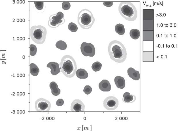
Figure 2. Atmospheric environment at the beginning of simulation.
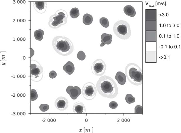
Figure 3. Atmospheric environment after 300 s.
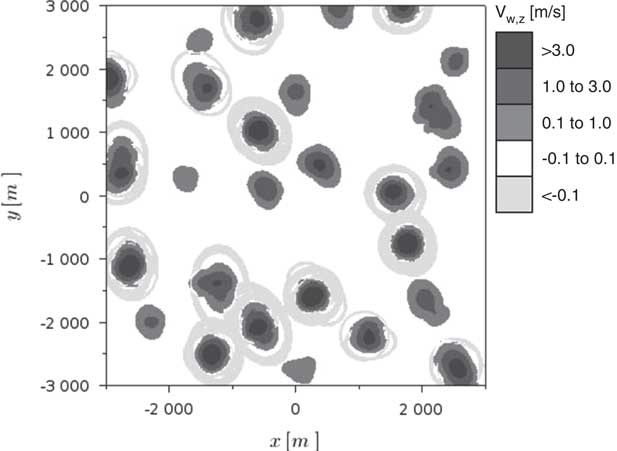
Figure 4. Atmospheric environment after 3300 s.
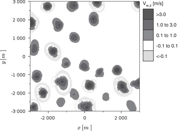
Figure 5. Atmospheric environment at the end of simulation.
The adopted controller parametres are summarised in Table 2. Some of them reflect airframe limitations (e.g. stall speed and control bounds), while others were selected according to practical considerations, like the 45 s (ΔT te N te ) sliding time window for retaining the estimated air vertical velocity data, which is analogous to the one used by Allen( Reference Allen 4 ) and Edwards( Reference Edwards 5 ) in test flights. In addition to that, several parametres were tuned during the simulations to obtain the desired closed loop behaviour (e.g. the weighting matrices). Note that the climb mode high-level controller works with a ΔT=2 s sampling time, updating the reference signals every ΔT ref =10 s. The related prediction horizon of 50 s (NΔT) has been found to be a good trade-off. Small values make the controller avoid crossing short downdraft zones to eventually reach the updraft core, or even prevent more aggressive manoeuvres (with associated instantaneous sink rate increment) that are sometimes necessary to centre a thermal. On the other hand, longer horizons imply proper centring performance, but also more computational effort. Regarding the lower level controllers, all of them adopt a ΔT=0.2 s sampling time and relatively short horizons, which has proven to yield accurate tracking of the set-points.
Table 2 Controller parametres used in the simulation

a Q and R are diagonal matrices.
b Used by all modes.
c Used by scan and climb modes.
The simulation started with the aircraft at a height of 1000m over co-ordinates (−2100 m, −2100 m) heading to the waypoint (2100 m, 2100 m). Figures 6 and 7 present the resultant trajectory in 2D and 3D format, respectively. A great part of the airspace was scanned in accordance with the waypoint calculation strategy used by the search mode. At the end of the simulation window, the UAV had just detected a thermal in a still unexplored area, around position (−1600 m, 250 m). It was able to keep safe altitudes during the entire flight (a minimum of 887m at 387 s), as indicated in Fig. 8.
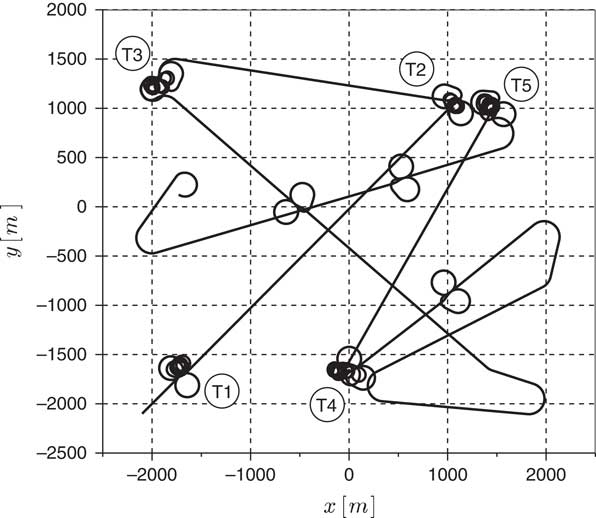
Figure 6. Flight path after 1 h – 2D view.
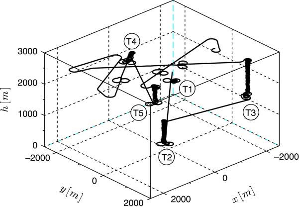
Figure 7. Flight path after 1 h – 3D view.
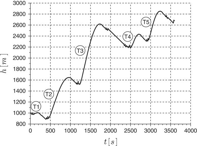
Figure 8. Height variation.
Figure 9 shows the operation mode status at each instant of time, where 1, 2 and 3 stand for search, scan and climb, respectively. It was switched 22 times and the climb mode engaged in five occasions (labels T1–T5 in Figs 6–9), with considerable atmospheric energy harvesting in the last four attempts. Further, in three opportunities (around 1875, 2330 and 3365 s), a thermal was encountered but the algorithm understood it was too weak and no circling was attempted. Table 3 summarises the controller overall and per stage (climb and scan legs only) performance. Notice that the flight terminated at a substantially higher altitude (a total gain of 1684 m), while the mean rate of climb during successful climbs varied from 0.8 m/s to 1.8 m/s, values that fall well within the typical range attained by manned sailplanes.
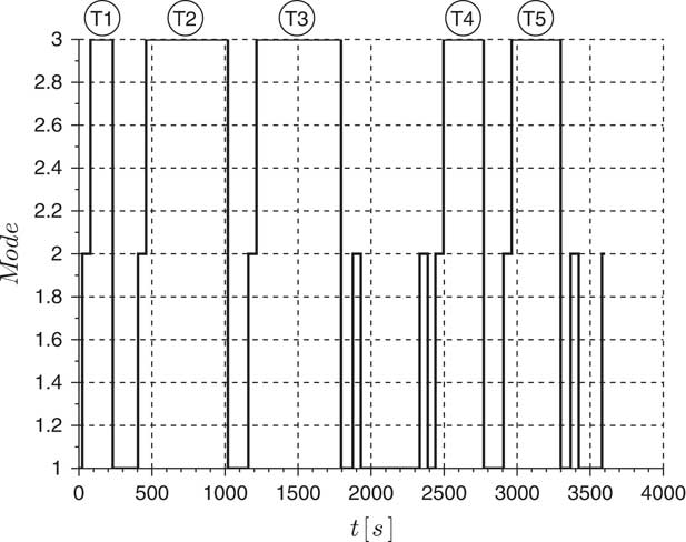
Figure 9. Active controller operation mode.
Table 3 Summary of soaring flight performance
a Thermal T1.
b Thermal T2.
c Thermal T3.
d Thermal T4.
e Thermal T5.
A detailed view of the flight path immediately before the climb mode latching as result of the encounter with the second thermal is presented in Fig. 10. The ‘8-shaped’ exploratory orbit imposed by the previously engaged scan mode adequately covered the updraft area, providing reasonable data to the first thermal estimate. Thereafter, the flight path converged to a circular trajectory around the core, as indicated in Fig. 11. It is worth mentioning that, about 6.5 min after the climb mode engagement (the instant of time shown in Fig. 11), the updraft intensity was considerably lower, indicating that it would soon be abandoned. Indeed, this trend is confirmed by Figs 12 and 13, which show the height and the total energy rate variation, respectively, from updraft encounter to the time when it was abandoned. After having reached the maximum value around 550 s, the mean energy rate is clearly decreasing with time as a result of the thermal weakening. The observed fluctuation in
 $$\dot{e}\left( t \right)$$
is mainly due to the fact that the environment is composed of non-circular updraft zones. For that reason, the optimal path is generally not a permanent flight condition, so the UAV crosses areas of different lift availability during each turn (Andersson et al(
Reference Andersson, Kaminer, Dobrokhodov and Cichella
7
) reported an analogous behaviour during flight test). Moreover, the constant control actions, required to track the reference trajectory, cause the vehicle drag to change, modifying the total energy rate, therefore, contributing to the phenomenon.
$$\dot{e}\left( t \right)$$
is mainly due to the fact that the environment is composed of non-circular updraft zones. For that reason, the optimal path is generally not a permanent flight condition, so the UAV crosses areas of different lift availability during each turn (Andersson et al(
Reference Andersson, Kaminer, Dobrokhodov and Cichella
7
) reported an analogous behaviour during flight test). Moreover, the constant control actions, required to track the reference trajectory, cause the vehicle drag to change, modifying the total energy rate, therefore, contributing to the phenomenon.
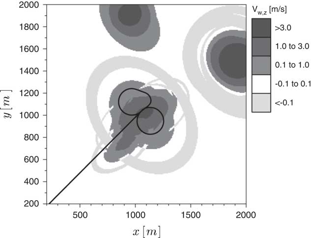
Figure 10. Flight path 55 s after the encounter with the second thermal.
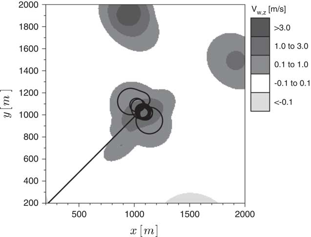
Figure 11. Flight path 445 s after the encounter with the second thermal.
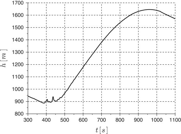
Figure 12. Height response during the encounter with the second thermal.
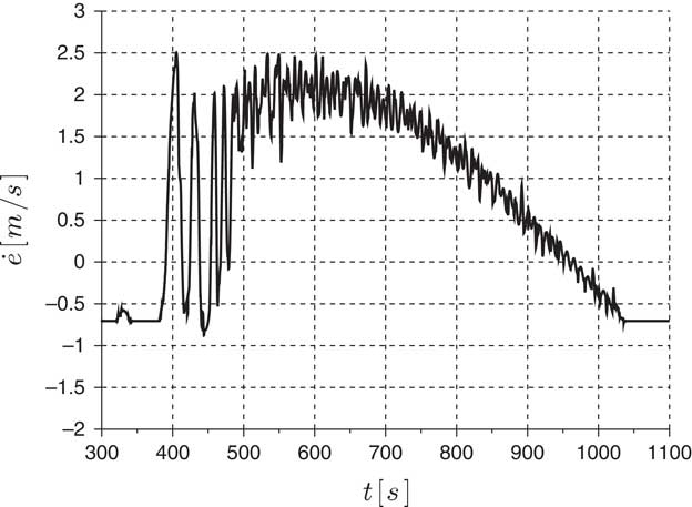
Figure 13. Total energy rate response during the encounter with the second thermal.
Figures 14 and 15 reveal how the airspeed and radius behaved during the exploration of the second thermal. The corresponding reference signals are also indicated, even though the two sets of curves are almost indistinguishable on the scale of the figures, except for a restricted zone around 435 s, which corresponds to the instant when the scan mode controller commanded the curve direction change. The set-point values remained constant at V scan = 110 km/h and r scan =120 m, while the plant response indicated a temporary deviation. Apart from that short interval, the low-level controllers were able to closely track the references. At approximately t=460 s, the climb mode was latched and from that moment on, the set-points were updated by the high-level MPC controller every 10 s, explaining the small steps seen in the responses. This feature is more noticeable in the case of Fig. 15, because the reference point for measuring the radius is also re-evaluated accordingly.
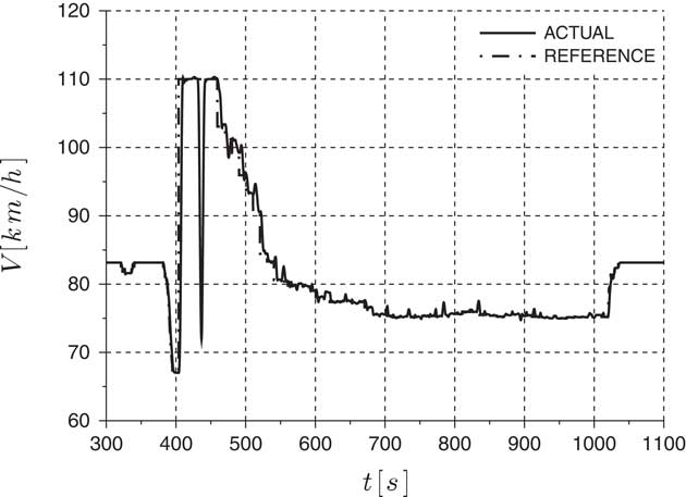
Figure 14. Airspeed response and set-point during the encounter with the second thermal.
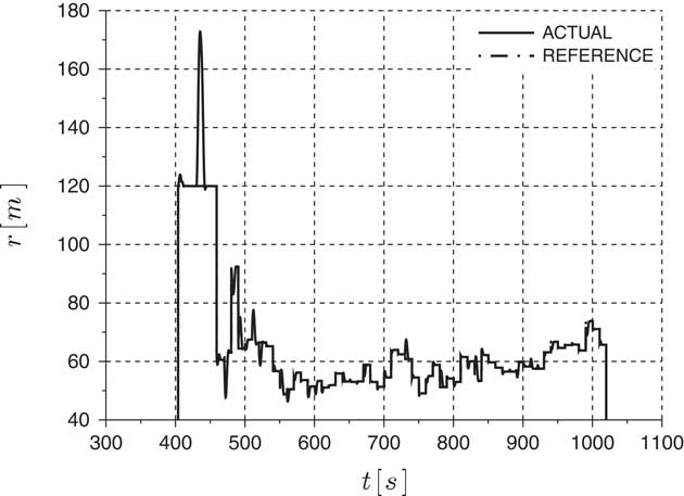
Figure 15. Radius response and set-point during the encounter with the second thermal.
As seen in Fig. 14, as soon as the climb mode was engaged, the guidance and control algorithm started to reduce the airspeed until a value slightly superior to the aircraft minimum sink velocity (see Table 1) was reached and maintained. At the same time, the radius decreased to values between 45 and 65m approximately. Possibly, flying faster at the beginning was preferred because reaching the updraft central region was more important than saving height. Moreover, the initial thermal environment evaluations tend to be less accurate, forcing the aircraft to seek every new estimated thermal core. It is important to point out that the imposed airspeed lower constraint (67 km/h, see Table 2) was activated at nearly 400s. This is due to MacCready’s rule implemented on the search mode controller, that commanded an airspeed decrease immediately after the UAV entered the positive climb zone of the thermal. Nevertheless, the stall speed limit was not crossed, clearly illustrating the natural way the constraints are treated by MPC schemes and its utility to autonomous soaring applications.
Figure 16 shows that the height response compares well to the high-level controller predictions throughout the initial climb phase within the second thermal. This validates both the internal model based on the simplified dynamics and the thermal estimation scheme. Note that even during the first seconds, when the radius and airspeed vary considerably and the aircraft is clearly flying in a non-permanent regime, the applied quasi-steady corrections to the sink rate lead to a relatively accurate prediction. As centring is progressively achieved, the discrepancies become smaller. However, a different situation is seen towards the end of the updraft life cycle, when the lift intensity is decreasing fast, according to the imposed sinusoidal rule. Since the thermal estimation procedure uses data related to the last 45 s, the predicted updraft strength and consequently the height gains are overestimated, exactly as indicated in Fig. 17. Possibly, the usage of time varying thermal models could minimise the disparities and improve the climbing predictions. Nevertheless, as noticeable in the figure, every 10 s, the high-level controller internal model is realigned. That operation, applied to the entire set of state variables, is fundamental to keep the predictor’s accuracy.
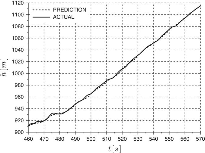
Figure 16. Comparison between actual and predicted height responses – second thermal centring.
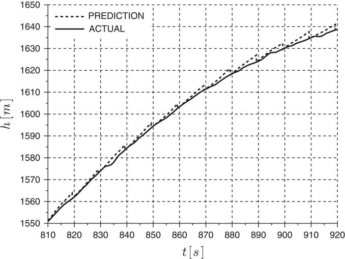
Figure 17. Comparison between actual and predicted height responses – end of second thermal life cycle.
A missed thermal situation is illustrated in Figs 18 and 19. The results of the total specific energy evaluation made during the preliminary scan manoeuvre were not enough to cross the imposed threshold, defined by the parametres
 $$\dot{e}_{{scan}} $$
and α
scan
(Table 2), as explained in Section 3.4. Thus, the updraft was considered unsuitable for climbing and the aircraft proceeded to the next calculated waypoint. It is important to add that the thermal was not vanishing, but still growing, a scenario normally considered ideal by glider pilots. Indeed, possibly one more turn would be sufficient for the climb mode to be latched. Therefore, it could be advantageous to somehow modify the scan algorithm in order to recognise the current thermal stage, allowing recently formed ones to be exploited.
$$\dot{e}_{{scan}} $$
and α
scan
(Table 2), as explained in Section 3.4. Thus, the updraft was considered unsuitable for climbing and the aircraft proceeded to the next calculated waypoint. It is important to add that the thermal was not vanishing, but still growing, a scenario normally considered ideal by glider pilots. Indeed, possibly one more turn would be sufficient for the climb mode to be latched. Therefore, it could be advantageous to somehow modify the scan algorithm in order to recognise the current thermal stage, allowing recently formed ones to be exploited.
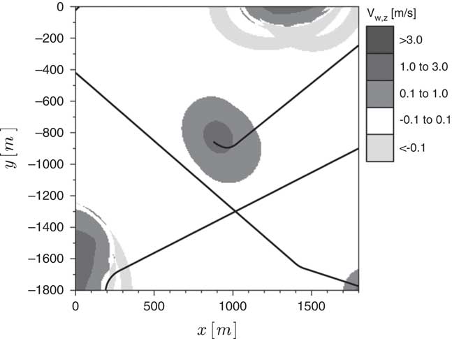
Figure 18. Flight path 5 s after the encounter with the second missed thermal.
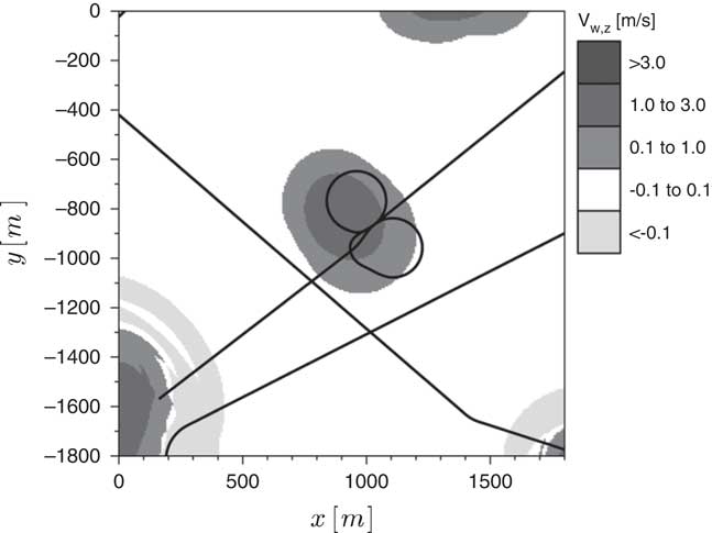
Figure 19. Flight path 100 s after the encounter with the second missed thermal.
Table 4 presents a summary of the algorithm computational performance. It refers to the proposed test case run on a 1.80 GHz quad-core CPU, 16 GB RAM personal computer executing Scilab version 5.5.0 under Ubuntu Linux 64 bits. The displayed time intervals encompass the entire set of operations needed for a single step, from the plant output measurements to the control signal generation.
Table 4 Required computation time
a Includes the thermal estimation and the high-level MPC run (see Fig. 1).
Thanks to the simplicity of the involved operations, the maximum recorded computation time when only the low-level control actions are carried out is roughly half the sampling time (ΔT=0.2 s). This is a promising result for a future real-time usage on flight hardware. However, possible complications arise when the full computations have to be performed, i.e. when the optimal reference trajectory has to be recalculated by the high-level MPC controller and the thermal parametres updated. According to the ΔT ref value in Table 2, this action is taken every 10 s when the climb mode is latched, having being repeated 194 times during the 1-h simulation. For those cases, Table 4 states that calculation times greater than the elementary 0.2 s sampling time were recorded (up to 1.04 s). Fortunately, there is a straightforward way to deal with that problem which requires only slight modifications on the algorithm. It consists in keeping the previously computed reference path until the current calculation is completed. In order to emulate that, the simulation whose results were presented throughout this section has been run with a fixed 1.2s lag in the high-level controller response. Comparisons with analogous runs without any lag have shown that the main impact is more aggressive control actions, once the set-points are suddenly updated and the controller ‘realises’ there is an error. Nevertheless, no significant closed-loop performance discrepancies could be noted. Furthermore, the same approach can also serve as a tool for handling infeasibility problems (so critical to MPC applications), since the previous reference solution can be used at least until the high-level controller prediction horizon elapses.
It is important to point out that the thermal identification process, i.e. the least squares fitting of the ellipsoid model, is responsible for approximately 30% of the calculation time per step. Thus, alternative regression algorithms for estimating the updraft field could be tested in the future to speed up the computations. In the same way, the NLP problem solution takes about 60% of the time. Although the LINCOA code worked successfully, it is not indicated for very large numbers of variables. Hence, the adoption of codes which are more suitable to high-dimensional NLP problems could further improve the performance.
5.0 CONCLUSION
The performed numerical simulations employing a 3 DOF model are the first step to demonstrate the feasibility of the proposed guidance and control strategy. According to the obtained results, a UAV running the developed algorithm, subsequently switching between the three different operation modes, would be able to explore a non-homogeneous time varying environment, identify, map, centre and climb in thermals without violating the aircraft performance limitations. In other words, energy from the convective phenomena which take place on the lower atmosphere could be successfully harvested without the help of complex onboard equipment for lift detection, resulting in endurance increase.
Some critical aspects of the proposed methodology have been tested and verified. Most notably, the simplified kinematic relations with quasi-steady sink corrections (the algorithm’s core) have proven to yield sufficiently accurate predictions. Therefore, the present MPC approach for autonomous soaring can serve as an alternative to existing schemes. Its main advantage is certainly the capability of producing simpler and smaller non-linear optimisation problems, thanks to the usage of explicit linear prediction schemes to the maximum extent possible. For instance, the climb mode high-level controller used in the test case of Section 4 requires a NLP problem with only 50 variables and 150 linear inequalities to be solved at each calculation step, covering a 50 s prediction horizon. If the differential constraints had to be explicitly imposed, for example by directly using the 3 DOF non-linear EOM for prediction, the number of variables would be much larger (by a factor of four approximately) and extra non-linear constraints would have to be considered. Hence, one concludes that the present methodology has the potential to facilitate the implementation of less complex, faster and more efficient codes, ultimately leading to straightforward integration on flight hardware. Indeed, the obtained computation times and adopted implementation strategies point to viable real-time operation.
Following this preliminary study, additional developments are currently in progress before moving towards flight testing.


