


Introduction
It was the Bronze Age; the revolutionary invention was the wheel that begot a chariot. Through the passage of time and advancement of technology, the chariot entered into the Industrial Age. Now it has many varieties in terms of brand, the source of energy, body style, and features like safety, comfortability, and entertainment. As a whole, a wide range of multi-attributed alternatives are generated according to the customer requirements. In the engineering point of view, it is termed as product design and development (Otto and Wood, Reference Otto and Wood2001; Zha et al., Reference Zha, Sriram and Lu2004). A successful product has to fulfill all the functional requirements and to be economical where the right choice of constituent material of a product from the wide range of materials takes the vital role (Pfeifer, Reference Pfeifer2009). The design is a sequential decision-making process that requires data where some degree of uncertainty always exists. The existence of a designer depends on the satisfaction of a customer. A designer and customer both are in the same situation of “which alternative” is to choose under uncertainty.
The aim of this paper is to investigate the “which” under uncertainty by implementing the Manhattan distance (Taxicab geometry) (Krause, Reference Krause1986) as a choice parameter in multi-attributed decision-making (MADM) framework to select the preeminent material (Fig. 1).
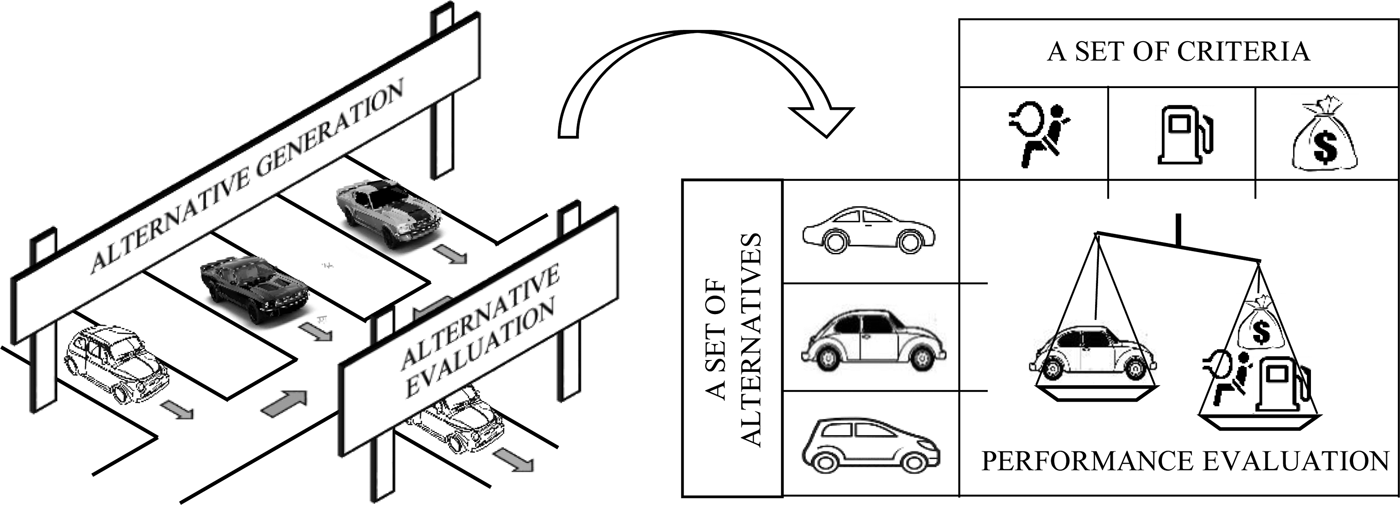
Fig. 1. Graphical multi-attributed decision-making framework.
Material selection
Material selection in machine design perspective can be delineated as the outcomes of the alternatives generation followed by the alternatives evaluation.
Alternatives generation
There is no one-way method to generate the alternatives. Significantly, from the Suh's design axioms (Suh, Reference Suh1990), alternatives can be generated by mapping the functional requirements with the design parameters (Dieter, Reference Dieter1983). Ashby (Reference Ashby1999) formalized the Suh's design axioms in a noetic way and proposed a chart known as Ashby's Chart to generate the potential materials under a specific condition. It can be regarded as a satisficing (Simon, Reference Simon, Bell, Raiffa and Taversky1988) model in the field of material selection in engineering design where he showed the performance of the machine elements is the function of the material properties. The chart is a log-log plot whose abscissa and ordinate are the material properties, but we are left in this chart with many alternatives or a set of potential alternatives. Due to the lack of information, uncertainty takes place in the design formulation and thereby alternative generation in material selection. Hazelrigg (Reference Hazelrigg2003) proposed an axiomatic framework based on Neuman–Morgenstern utility axioms to evaluate the alternatives under uncertainty. It is known as decision-based design framework where the alternatives are evaluated by their expected utility values to ensure a rational choice (Wassenaar and Chen, Reference Wassenaar and Chen2003; Das et al., Reference Das, Bhattacharya and Sarkar2016). However, a structured method is required, which is germane to the material selection under uncertainty to evaluate the alternatives and thereby to raise the preeminent one.
Alternatives evaluation
Alternatives are generally evaluated in the domain of multiple-criteria decision analysis (MCDA) where the alternatives are described in terms of evaluative criteria. MCDA methods are further categorized as:
• MADM where the decision space is explicitly known and discrete.
• Multi-objective decision-making (MODM) where the decision space is continuous.
The sole attention of this paper is about the MADM framework. MADM approaches are already well demonstrated that addresses the uncertainty by considering a set of alternatives with uncertain values for the attributes or criteria of the alternatives (Wallenius et al., Reference Wallenius, Dyer, Fishburn, Steuer, Zionts and Deb2008; Shahinur et al., Reference Shahinur, Sharif Ullah, Noor-E-Alam, Haniu and Kubo2017). The basic steps in all MADM approaches are generally considered as:
• Decision matrix is the discrete decision space where a finite set of alternatives is expressed by its performance ratings in multiple attribute or criteria.
• Weightage or priority is assigned to each criterion according to the design requirements to satisfy the customer's demands and desires. Analytical hierarchy process (AHP) (Mujgan et al., Reference Mujgan, Ozdemir and Gasimov2004; Hu et al., Reference Hu, Wang, Wang, Wang and Zhang2014), fuzzy AHP (Chan et al., Reference Chan, Kumar, Tiwari, Lau and Choy2008), digital logic (DL), modified DL (Dehghan-Manshadi et al., Reference Dehghan-Manshadi, Mahmudi and Abedian2007), and entropy are some popular methods for priority distribution (Jahan et al., Reference Jahan, Mustafa, Sapuan, Ismail and Bahraminasab2012b).
• Normalization is the process by which the performance ratings measured in the different unit are converted into a common unit. Vector normalization based on Euclidean distance, standardization based on standard deviation, and feature scaling based on the difference between the best and worst values are widely used (Hatush and Skitmore, Reference Hatush and Skitmore1998; Opricovic and Gwo-Hshiung, Reference Opricovic and Gwo-Hshiung2004; Rao and Patel, Reference Rao and Patel2010; Girubha and Vinodh, Reference Girubha and Vinodh2012).
• Overall performance analysis that assigns the overall performance rating to each alternative and the alternatives are ranked accordingly. According to the nature of the mathematical models used in the analysis, the MADA methods are named (Shanian et al., Reference Shanian, Milani, Carson and Abeyaratne2008; Peng and Xiao, Reference Peng and Xiao2013; Mousavi-Nasab and Sotoudeh-Anvari, Reference Mousavi-Nasab and Sotoudeh-Anvari2017).
Compiling the above-mentioned four steps, various MADM models are formed. There is an ample literature where varieties of MADM methods are discussed, modified, and applied in the field of material selection. Shahinur et al. (Reference Shahinur, Sharif Ullah, Noor-E-Alam, Haniu and Kubo2017) judiciously introduced the fuzzy logic to select the material for vehicle body and the aluminum alloys are chosen as the best materials. Cryogenic storage tank materials are analyzed by WPM (Dehghan-Manshadi et al., Reference Dehghan-Manshadi, Mahmudi and Abedian2007), TOPSIS (Jahan et al., Reference Jahan, Bahraminasab and Edwards2012a), MOORA (Karande and Chakraborty, Reference Karande and Chakraborty2012), Fuzzy logic (Khabbaz et al., Reference Khabbaz, Manshadi, Abedian and Mahmudi2009), and the preeminent material is considered as Austenitic steel (SS 301-FH). Flywheel materials are evaluated by TOPSIS (Jee and Kang, Reference Jee and Kang2000), VIKOR, ELECTRE (Chatterjee et al., Reference Chatterjee, Athawale and Chakraborty2009), and TOPSIS (Jahan et al., Reference Jahan, Bahraminasab and Edwards2012a) and the analyses show the best material is Kevler 49-epoxy FRP. Gear materials are divisioned by Extended PROMETHEE II (Chatterjee and Chakraborty, Reference Chatterjee and Chakraborty2012), TOPSIS (Milani et al., Reference Milani, Shanian, Madoliat and Nemes2005), and MULTIMOORA (Hafezalkotob et al., Reference Hafezalkotob, Hafezalkotob and Sayadi2016) and raise the best material as Carburised steel. Metallic bipolar plate materials are interpreted by VIKOR (Rao, Reference Rao2008) and TOPSIS (Shanian and Savadogo, Reference Shanian and Savadogo2006) and the optimal choice shows the Austenitic stainless steel 316. Meanwhile, with time and the advancement of technology, new materials are being used besides the traditional materials. For example, shape memory alloy (smart material) that can memorize the shape at various operating conditions and behave accordingly. Unlike traditional MADM approaches, Huang (Reference Huang2002) introduced a series of performance index charts under various operating conditions to select the preeminent material for actuators and suggested the NiTi popularly known as Nitinol as a good choice.
From the above discussion, it can be concluded that the TOPSIS and VIKOR are widely used. In most of the cases, different types of normalization process are suggested and implemented (Fayazbakhsh et al., Reference Fayazbakhsh, Abedian, Manshadi and Khabbaz2009), but the basic structure of overall performance analysis of the alternatives in all processes is same. Cables et al. (Reference Cables, Lamata and Verdegay2016) proposed a method, reference ideal method where the only “ideal point” is considered as a reference point (in case of TOPSIS, there is an “ideal point” and a “negative ideal point”) and the outcomes are compared with TOPSIS and VIKOR methods. Lourenzutti and Krohling (Reference Lourenzutti and Krohling2014) introduced the Hellinger distance in TOPSIS (H-TOPSIS), whereas the original TOPSIS is based on Euclidean distance.
Gap analysis and aim
From the above discussion, some of the methods (Lourenzutti and Krohling, Reference Lourenzutti and Krohling2014; Cables et al., Reference Cables, Lamata and Verdegay2016) can be regarded to certain extent as a nearest neighbor search (NNS) approach (Barrena et al., Reference Barrena, Jurado, Neila and Pachon2010). NNS is the finding of a point (a) in a given set which is nearer to a reference point or query point (q) in a multi-dimensional Euclidean space. In the above-mentioned TOPSIS-based methods, the closeness or nearness between two points is decided by a ratio that lies between 0 and 1 where the higher value dictates the close proximity. All the methods are structured with strong mathematical background, but if we consider the alternative as a point in the metric space, there is some lack of spatial relationship evidence from “closeness” point of view. From a mathematical point of view, the closeness between two points can be described as a distance parameter, d(a, q) → 0 as a → q (Arkhangel'skii and Fedorchuk, Reference Arkhangel'skii, Fedorchuk and Gamkrelidze1990).
At this point, very specifically, the aim of this paper is to select the preeminent material in design based on NNS on the basis of d(a, q) → 0 in the Cartesian plane under MADM framework through the eyes of TOPSIS. If the points (alternatives) are mapped in the two-dimensional plane, then we can easily visualize and compare the points with the query point. The designers rather enjoy the spatial relationship which gives a confidence and courage under uncertainty.
Proposed NNS-based material selection in the Cartesian plane
The NNS is generally pronounced in the field of machine learning, pattern recognition, geometrical information systems, and many others (Papadopoulos and Manolopoulos, Reference Papadopoulos and Manolopoulos2005; Moghtadaiee and Dempster, Reference Moghtadaiee and Dempster2015). It deals with spatial data in an effective and efficient way. The data can be characterized as points or lines or higher entities oriented in two-dimensional or multi-dimensional space. The scenario is the same in nature in the sense of material selection where the material is considered as an n-dimensional point in the above-mentioned MADM methods. There is a wide range of NNS methods.
The proposed approach does not consider the traditional NNS methods, but the basic definition of the NNS, that is, searching the nearness of a set of points (a i=1,2,…,m) to a query point (q) by means of a distance parameter in n-dimensional Euclidean space (a i,q ∈ ℝn) shown in Figure 2. From the material selection point of view, the absolute nearness or similarity between a i (alternatives) and q (reference alternative) depends upon the length of the position vectors  $\lpar {\vert {\overrightarrow {oa_i}} \vert \comma \,\vert {\overrightarrow {oq}} \vert } \rpar $ and the angle between the vectors (θ i). Cosine similarity is a popular approach (Kou and Lin, Reference Kou and Lin2014; Xia et al., Reference Xia, Zhang and Li2015) to find the θ i that investigates the similarity among alternatives and given by,
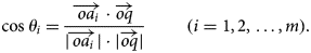 $$\cos \theta _i = \displaystyle{{\overrightarrow {oa_i} \cdot \overrightarrow {oq}} \over {\vert {\overrightarrow {oa_i}} \vert \cdot \vert {\overrightarrow {oq}} \vert }} \quad \quad {\rm \;} (i = 1\comma \,2\comma \, \ldots\comma \, m).$$
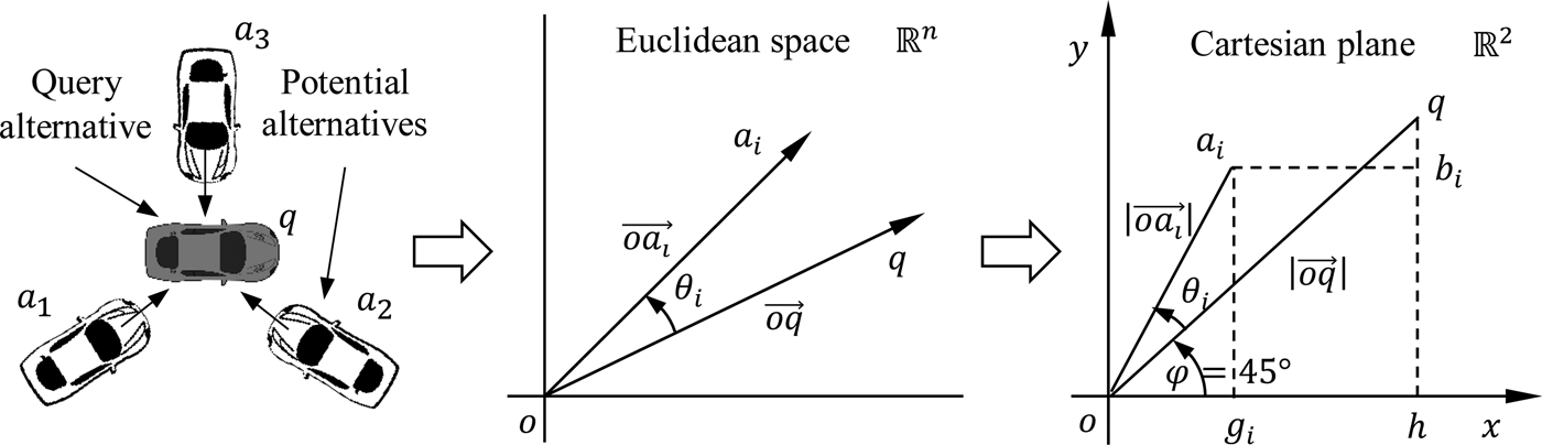
Fig. 2. Spatial representation of alternatives and choice parameter.
Therefore, the comparison between a i and q is the function of the length and orientation of the alternatives and should be mapped in the Cartesian plane  $\lpar {\lpar {\vert {\overrightarrow {oa_i}} \vert \comma \,\theta_i\comma \,\vert {\overrightarrow {oq}} \vert } \rpar :{\rm {\open R}}^n \to {\rm {\open R}}^2} \rpar $ in respect of the query vector to investigate the exact nearness between a i and q by means of the distance parameter (Fig. 2). Actually, these distance parameters are the dissimilarity functions of the alternatives and the less value of the dissimilarity function dictates the choice which is very nearer to the query point. Now the question is that which distance parameter should be considered, Euclidean distance (l 2 norm) or Manhattan distance (l 1 norm). In Cartesian plane, the Manhattan distance is the sum of the projected length of a Euclidean distance along the axes. The proximity of any two points depends upon the adjustment of the coordinates along the axes which preserve the absolute similarity information. Therefore, our decision favors the Manhattan distance. From the Cartesian plane in Figure 2, the coordinates of a i and q are
  $a_i = \lpar {\vert {\overrightarrow {oa_i}} \vert \cos \lpar {\theta_i + \varphi} \rpar \comma \,\vert {\overrightarrow {oa_i}} \vert \sin \lpar {\theta_i + \varphi} \rpar } \rpar $ and
  $q = \lpar {\vert {\overrightarrow {oq}} \vert \cos \varphi\comma \, \vert {\overrightarrow {oq}} \vert \sin \varphi} \rpar $. The Manhattan distance between a i and q is given by,
 $$d_{\rm M}(a_i\comma \,q) = \overline {a_ib_i} + \overline {b_iq} {\rm \;} \quad \quad i = 1\comma \,2\comma \, \ldots\comma \, m\comma \,$$
where
 $$\overline {a_ib_i} = \vert {\vert {\overrightarrow {oq}} \vert \cos \varphi - \vert {\overrightarrow {oa_i}} \vert \cos \lpar {\theta_i + \varphi} \rpar } \vert \comma \, $$
 $$\overline {b_iq} = \vert {\vert {\overrightarrow {oq}} \vert \sin \varphi - \vert {\overrightarrow {oa_i}} \vert \sin \lpar {\theta_i + \varphi} \rpar } \vert. $$
 The most favorable orientation of  $\vert {\overrightarrow {oq}} \vert $ in Cartesian plane is the equi-inclination with the axes, that is, φ = 45° that gives the optimal position of q and the maximum equivalent Manhattan distance of the length
  $\vert {\overrightarrow {oq}} \vert \; \lpar {d_{\rm M}\lpar {o\comma \,q} \rpar = \overline {oh} + \overline {hq}} \rpar$. In the Cartesian plane (Fig. 2), the line
  $\overline {oa_i} $ can be either any side of
  $\overline {oq} $ and θ i may or may not be greater or less than 45°, but the ultimate Manhattan distance (d M(a i, q)) will be the same in all cases and the generalized Manhattan distance between a i and q following the expressions (2) to (4) is given by,
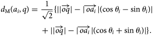 $$\eqalign{d_{\rm M}\lpar {a_i\comma \,q} \rpar =\;& \displaystyle{1 \over {\sqrt 2}} \lcub {\vert {\vert {\overrightarrow {oq}} \vert - \vert {\overrightarrow {oa_i}} \vert \lpar {\cos \theta_i - \sin \theta_i} \rpar } \vert} \cr \;&+ {\vert {\vert {\overrightarrow {oq}} \vert - \vert {\overrightarrow {oa_i}} \vert \lpar {\cos \theta_i + \sin \theta_i} \rpar } \vert } \rcub .}$$
 In the Cartesian plane (Fig. 2), the line  $\overline {oa_i} $ can be either any side of
  $\overline {oq} $ and θ i can be >45°, but the ultimate Manhattan distance (d M(a i, q)) will be the same. The minimum value of the expression (5) addresses the preeminent alternative.
Implementation of the proposed model in the MADM framework
A set of alternatives (A) with performance ratings (D) is decided according to the design requirements. Performance is the measure of effectiveness in the form of attributes (E). Attributes are set according to the demands and desires of the design requirements and can be split up in benefit and cost attributes. The steps are followed to capture the preeminent alternative:
Step 1: A set of alternatives with performance ratings in the form of attributes
(6) $$A = \lcub { {a_i} \vert i = 1\comma \,2\comma \, \ldots\comma \, m} \rcub \comma \,$$(7)$$E = \bigg\{ { {e_j} \vert \underbrace{{\mathop {\,j = 1\comma \,2\comma \, \ldots\comma \, n - r}\limits_{}}}_{{{\rm benefit\; attribute}}};\underbrace{{\,j = n - r + 1\comma \, \ldots\comma \, n}}_{{{\rm cost\; attribute}}}} \bigg\} \comma \,$$(8)$$D = \lcub { {d_{ij}} \vert i = 1\comma \,2\comma \, \ldots\comma \, m;\;j = 1\comma \,2\comma \, \ldots\comma \, n} \rcub .$$
Step 2: Weightage to the attributes
(9)$$W = \lcub { {w_j} \vert j = 1\comma \,2\comma \, \ldots\comma \, n} \rcub .$$Step 3: Normalization of the performance rating matrix
(10)$$r_{ij} = \displaystyle{{d_{ij}} \over {\sqrt {\mathop \sum \nolimits_{i = 1}^m d_{ij}^2}}} \quad \quad {\rm \;} j = 1\comma \,2\comma \, \ldots\comma \, n.$$Step 4: Weighted normalization of the performance rating matrix
(11)$$x_{ij} = r_{ij} \cdot w_j = \displaystyle{{d_{ij}} \over {\sqrt {\mathop \sum \nolimits_{i = 1}^m d_{ij}^2}}} \cdot w_j\quad \quad {\rm \;} j = 1\comma \,2\comma \, \ldots\comma \, n.$$Step 5: Query alternative with performance ratings
(12)$$\eqalign{&q = \lcub { {y_j\lpar {\max x_{ij}} \rpar } \vert j = 1\comma \,2\comma \, \ldots\comma \, n - r;{\rm \;}} \cr &{{y_j\lpar {\min x_{ij}} \rpar } \vert j = n - r + 1\comma \, \ldots\comma \, n} \rcub .}$$Step 6: Mapping of the alternatives and query alternative in Euclidean space
(13)$$\overrightarrow {oa_i} = \mathop \sum \limits_{\,j = 1}^n x_{ij} \cdot \widehat{{e_j}}\quad \quad i = 1\comma \,2\comma \, \ldots\comma \, n\comma \,$$(14)$$\vert {\overrightarrow {oa_i}} \vert = \sqrt {\mathop \sum \limits_{\,j = 1}^n x_{ij}^2} \quad \quad i = 1\comma \,2\comma \, \ldots\comma \, n\comma \,$$(15)$$\overrightarrow {oq} = \mathop \sum \limits_{\,j = 1}^n y_j \cdot \widehat{{e_j}}\quad \quad i = 1\comma \,2\comma \, \ldots\comma \, n\comma \,$$(16)$$\vert {\overrightarrow {oq}} \vert = \sqrt {\mathop \sum \limits_{\,j = 1}^n y_j^2}. $$Step 7: Cosine similarity following the expressions (1), (14), and (16)
(17)$$\cos \theta _i = \displaystyle{{\mathop \sum \nolimits_{\,j = 1}^n x_{ij} \cdot y_j} \over {\sqrt {\mathop \sum \nolimits_{\,j = 1}^n x_{ij}^2} \cdot \sqrt {\mathop \sum \nolimits_{\,j = 1}^n y_j^2}}} \quad \quad i = 1\comma \,2\comma \, \ldots\comma \, m{\rm \comma \,} $$(18)$$\sin \theta _i = \sqrt {1 - {\cos} ^2\theta _i} \quad \quad i = 1\comma \,2\comma \, \ldots\comma \, m{\rm \;} {\rm.} $$Step 8: Calculation of Manhattan distance following the expressions (2)–(4), (14), (16)–(18) or directly from the expressions (5), (14), (16)–(18)
(19)$$\eqalign{d_{\rm M}\lpar {a_i\comma \,q} \rpar =& \displaystyle{1 \over {\sqrt 2}} \lcub {\vert {\vert {\overrightarrow {oq}} \vert - \vert {\overrightarrow {oa_i}} \vert \lpar {\cos \theta_i - \sin \theta_i} \rpar } \vert} \cr &{+ \vert {\vert {\overrightarrow {oq}} \vert - \vert {\overrightarrow {oa_i}} \vert \lpar {\cos \theta_i + \sin \theta_i} \rpar } \vert } \rcub {\rm \;} {\rm.}} $$


The alternatives are ranked according to the minimum value of the Manhattan distance (d M(a i=1,2,…m, q)). The steps followed and the respective input/output of the proposed method are shown in Figure 3.
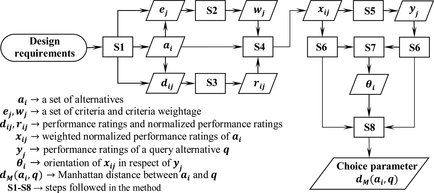
Fig. 3. Nearest neighbor search-based material selection flow diagram.
Case study 1: cryogenic storage tank
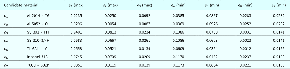
The cryogenic storage tank is also referred to cryogenic storage dewar (named after James Dewar, who first introduced liquid hydrogen and oxygen storage) is basically a double-walled vacuum/super-insulators vessel shown in Figure 4. It carries the liquid nitrogen, oxygen, hydrogen, argon, and helium gas with <110 K/−163 °C temperature. Liquid hydrogen has already been accepted as an excellent energy source. It is non-toxic and extremely environmentally benign as water is only the exhaust product when it is converted into the energy. The choice of material in cryogenic tank design is generally dictated by safety and economy. In case of cryogenic tank, the main issue is the safety factors and the design requirements under the consideration of low-temperature embrittlement can be stated as (Flynn, Reference Flynn2005; Farag, Reference Farag2014):
• Fracture toughness: The boiling temperature of liquid nitrogen gas is about −196°C or liquid hydrogen gas is about −253°C. At this temperature, the materials lose their ductile behavior and become brittle in nature. Therefore, materials should be sufficiently tough to resist the brittle fracture. The metals having face-centered cube (fcc) lattice are suitable because of their insensitiveness at low temperature. Copper, nickel, all of the copper–nickel alloys, aluminum and its alloys, and the austenitic stainless steels that contain more than approximately 7% nickel are suitable for designing any cryogenic storage tank (Flynn, Reference Flynn2005).
Fig. 4. Cryogenic storage tank and application.
• Heat transfer: The flow of heat through the wall of the cryogenic tank is generally conduction type. Materials having low thermal conductivity are preferable.
• Thermal stress: Due to the low temperature, the inner wall is subjected to a contraction that causes thermal stresses. Therefore, materials having a low coefficient of thermal expansion are suitable.
• Thermal diffusivity: Perfect thermal insulation is not possible practically. Materials should be chosen that they can release the heat as quickly as possible. Diffusivity measures the rate of transfer of heat, which is inversely proportional to the specific heat of the materials.
• Transportation: Materials having lower specific gravity is suitable for transportation.

From the above-mentioned discussion and MADM point of view, all attributes can be categorized as:
• Benefit attribute: Toughness index (e 1); yield stress (e 2); Young's modulus (e 3);
• Cost attribute: Specific gravity (e 4); coefficient of thermal expansion (e 5); thermal conductivity (e 6); specific heat (e 7).
Following the expressions (6)–(8), some of the candidate materials under uncertainty having fcc lattice are tabulated in Table 1 with their performance ratings. The relative weights to the attributes in expression (9) are assigned following the previous works (Dehghan-Manshadi et al., Reference Dehghan-Manshadi, Mahmudi and Abedian2007; Jahan et al., Reference Jahan, Bahraminasab and Edwards2012a, Reference Jahan, Mustafa, Sapuan, Ismail and Bahraminasabb; Karande and Chakraborty, Reference Karande and Chakraborty2012) and given by,
 $$w_{\,j = 1\comma \,2\comma \, \ldots\comma \, n} = [0.28\comma \,{\rm \;} 0.14\comma \,{\rm \;} 0.05\comma \,{\rm \;} 0.24\comma \,{\rm \;} 0.19\comma \,{\rm \;} 0.05\comma \,{\rm \;} 0.05].$$
Table 1. Performance ratings matrix (d ij) of case study 1

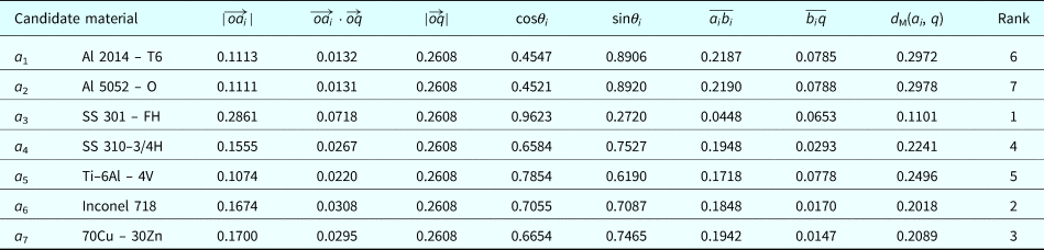
The weighted normalized performance ratings are tabulated in Table 2 following the expressions (10)–(11) and (20). From Table 2 and following the expression (12), the query alternative with performance ratings is given by,
 $$q = [0.2401\comma \,{\rm \;} 0.0813\comma \,{\rm \;} 0.0269\comma \,{\rm \;} 0.0369\comma \,{\rm \;} 0.0394\comma \,{\rm \;} 0.0012\comma \,{\rm \;} 0.0106].$$
Table 2. Weighted normalized performance ratings matrix (x ij) of case study 1
The overall performances of the alternatives are evaluated through the expressions (13)–(19) and (21) and tabulated in Table 3.
Table 3. Overall performance evaluation of case study 1
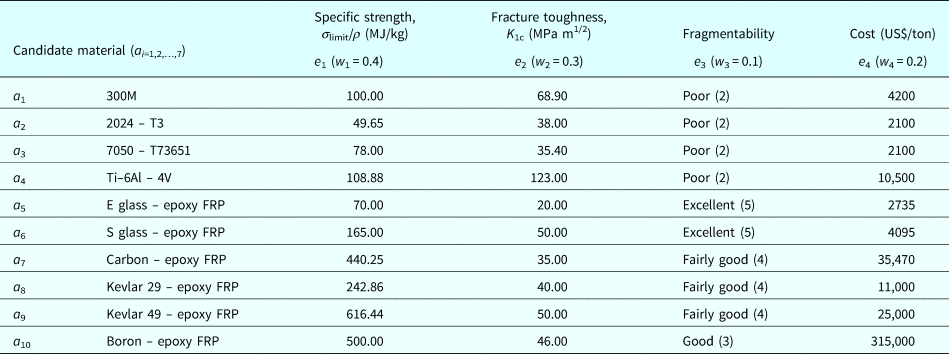
Case study 2: flywheel
The flywheel is an energy storage device used to maintain the minimum fluctuation of speed of a machine. Energy density, that is, ratio of the energy (e) and mass (m) is an important parameter used to qualify the energy storage device. The energy density is proportional to the ratio between maximum stress (σ u) the material can withstand and its density (ρ) (Genta, Reference Genta1985; Ashby, Reference Ashby1999) given by,
 $$\displaystyle{e \over m} = K \cdot \displaystyle{{\sigma _{\rm u}} \over \rho} {\rm \comma \,} $$
where K is known as the “shape factor” that depends on the geometrical configuration of the flywheel, and the choice of flywheel material depends on the specific strength (σ u/ρ). Composite materials are widely used due to its excellent specific strength. As the flywheel is subjected to the cyclic loading, the fatigue strength (σ limit) is considered instead of ultimate strength (σ u) (Jee and Kang, Reference Jee and Kang2000; Chatterjee et al., Reference Chatterjee, Athawale and Chakraborty2009).
Another important phenomenon is about the burst containment which is associated with the rotor. All materials have a fatigue life when they are subjected to cyclic loading or may have inconsistencies in the structure and the fracture may take place even below the strength limit. In some literature (Jee and Kang, Reference Jee and Kang2000), this fracture phenomenon is addressed by the ratio (K 1c/ρ) of fracture toughness (K 1c) and density (ρ), but there is no clear explanation of choosing density in fracture toughness. According to Griffith crack theory, the critical strain energy release rate (G 1c) that propagates the crack is given by (Broek, Reference Broek1984),
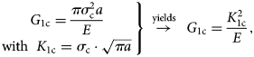 $$\left. {\matrix{ {G_{1{\rm c}} = \displaystyle{{\pi \sigma _{\rm c}^2 a} \over E}} \cr {{\rm with\; \; }K_{1{\rm c}} = \sigma _{\rm c} \cdot \sqrt {\pi a} } \cr } } \right\}{\rm \; }\mathop \to \limits^{{\rm yields}} {\rm \; \; }G_{1{\rm c}} = \displaystyle{{K_{1{\rm c}}^2 } \over E}{\rm ,}$$
where a is the half crack length (2a), σ c is the critical stress at which the fracture takes place and K 1c is known as the critical stress intensity factor or popularly fracture toughness. We would like to consider K 1c as a material selection attribute instead of K 1c/ρ. If the fracture happens, the wheel breaks up into the number of fragments and the kinetic energy of the wheel is transferred to the surrounding through these fragments that cause the damage to the system. In case of monolithic metal, the number of fragments is three or four, whereas for composite materials, there are many tiny fragments. On that ground, the composite materials are the better choice. One of the popular materials for the flywheel is Kevlar but it is costly. However, following the previous literature (Jee and Kang, Reference Jee and Kang2000), the specific strength (σ limit/ρ), fracture toughness to density ratio (K 1c), fragmentability, and cost are considered as material attributes for the flywheel. All attributes can be summarized as:
• Benefit attribute: specific strength (e 1); fracture toughness (e 2); fragmentability (e 3);
• Cost attribute: cost (e 4).
Some of the potential materials under uncertainty with their performance ratings are tabulated in Table 4 where basically Al alloys, Ti alloys, and Composite materials have been considered. Some material attributes are rather ordinal like fragmentability, creep resistance, or corrosion resistance and can be converted into cardinal by following the five-point Likert scale (Likert, Reference Likert and Woodworth1932) as: very weak – 1; weak – 2; average – 3; good – 4; excellent – 5. The priority to the attributes is assigned following the previous works (Jee and Kang, Reference Jee and Kang2000; Chatterjee et al., Reference Chatterjee, Athawale and Chakraborty2009) and given by,
 $$w_{\,j = 1\comma \,2\comma \, \ldots\comma \, n} = [0.4\comma \,{\rm \;} 0.3\comma \,{\rm \;} 0.1\comma \,{\rm \;} 0.2].$$
Table 4. Performance ratings matrix (d ij) of case study 2
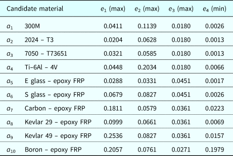
Following the same steps as case study1, the weighted normalized performance ratings are tabulated in Table 5 and the query alternative with performance ratings is given by,
 $$q = [0.2536\comma \,{\rm \;} 0.2034\comma \,{\rm \;} 0.0451\comma \,{\rm \;} 0.0013].$$
Table 5. Weighted normalized performance ratings matrix (x ij) of case study 2
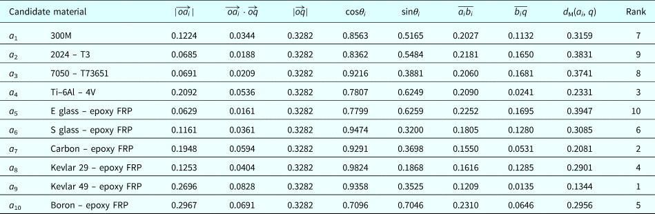
The overall performances of the alternatives are systematized in Table 6 according to steps 6–7 formalized in the proposed framework.
Table 6. Overall performance evaluation of case study 2
Results and discussion
In this analysis, the material properties are considered as discrete and average, but these are rather variable in nature. The true value cannot be known precisely (aleatory uncertainty). As the material selection is initiated at the conceptual stage of the design process, there is a further scope to analyze the suitability of the chosen material at the embodiment stage.
Cryogenic storage tank: For low temperature, <−163°C, the fcc materials are widely used. The austenitic steel SS 301 – FH is ranked 1 material in Table 3, which is a consistent result with the previous works and real-world practice. Austenitic steel still now is very popular and widely used liquid nitrogen or hydrogen storage tank (Godula-Jopek et al., Reference Godula-Jopek, Jehle and Wellnitz2012). Now it is the time to check the consistency of the ranking of the materials in Table 3 with previous works as:
Proposed method with vector normalization: 6-7-1-4-5-2-3;
MOORA with linear normalization (Karande and Chakraborty, Reference Karande and Chakraborty2012): 7-6-1-4-5-3-2;
WPM with non-linear normalization (Dehghan-Manshadi et al., Reference Dehghan-Manshadi, Mahmudi and Abedian2007): 5-7-1-4-2-3-6;
TOPSIS with target-based normalization (Jahan et al., Reference Jahan, Bahraminasab and Edwards2012a, Reference Jahan, Mustafa, Sapuan, Ismail and Bahraminasabb): 4-5-1-6-2-3-7.
Sometimes the second option is very important in the ranking. In Dehghan-Manshadi et al. (Reference Dehghan-Manshadi, Mahmudi and Abedian2007); Jahan et al. (Reference Jahan, Bahraminasab and Edwards2012a, Reference Jahan, Mustafa, Sapuan, Ismail and Bahraminasabb), the titanium alloy (Ti-6Al-4V) got second rank. Ti-6Al-4V is excellent in the aerospace industry, but for low-temperature embrittlement cases, titanium alloys are very weak (Flynn, Reference Flynn2005), whereas Inconel is a good alternative than titanium alloy as a cryogenic storage tank material.
Flywheel: The result in Table 6 gives some interesting points and a clear delineation of past and present. As the technology is changing rapidly, new challenging alternatives are taking place in the market, despite being costly a designer or decision maker bends toward the composite materials due to its excellent specific strength. The ranking in Table 6 is compared with the previous works as:
Proposed method: 7-9-8-3-10-6-2-4-1-5;
TOPSIS (Jee and Kang, Reference Jee and Kang2000): 5-9-7-6-8-3-4-2-1-10;
ELECTRE-II (Chatterjee et al., Reference Chatterjee, Athawale and Chakraborty2009): 10-9-8-6-7-3-2-4-1-5;
VIKOR (Chatterjee et al., Reference Chatterjee, Athawale and Chakraborty2009): 9-10-8-6-7-5-2-4-1-3.
There is no confusion about ranked 1 material, Kevlar 49 due to its excellent specific strength and consistent with the real-world practice (Genta, Reference Genta1985). Carbon-epoxy FRP also holds the second position in all methods. Composite materials reinforced with glass fiber, aramid, or carbon are similar in specific strength point of view and the choice among them differs by their cost mainly.
It is the versatility of the MADM approaches blended with mathematics and cognitions that different decision-making methods yield different rankings considering the same input data. Material selection takes place at the earliest stage of the design process when there is a lack of information and variability in the available information in the decision space. Under these circumstances, the proposed method gives a confidence in visualizing (geometrical) point of view and courage in ranking consistency point of view as compared with other rankings.
Conclusions
Engineering design is the judicious trade-off among shape, materials, and manufacturing that requires a wide range of decisions. Decision-making in engineering design allocates all the resources optimally while fulfilling the design objectives within economic constraints, quality constraints, safety constraints, environmental constraints, etc., under uncertainty.
To ensure an optimal choice, the problem should be precisely structured according to the decision requirements. In this paper, a simplified spatial approach is proposed to select the preeminent material by Manhattan distance along with the cosine similarity. In this approach, we can visualize the impact of the selection process. One may conclude, why not directly the Manhattan distance without considering the cosine similarity as given by,
 $$d_{\rm M}\lpar {a_i\comma \,q} \rpar = \mathop \sum \limits_{\,j = 1}^n \vert {x_{ij} - y_j} \vert \quad \quad i = 1\comma \,2\comma \, \ldots m.$$
In this case, for example, a cryogenic storage tank, the ranking will be changed as 6-7-1-4-2-3-5, but the rank 1 (austenitic steel SS 301 – FH) will be unchanged and the titanium alloy (Ti-6Al-4V) holds the rank 2. Whatever the methods, if the methods have definite logic, the fittest materials will be always survived, but there should have some consistency among the rankings inside a particular method. Inconel is much better than titanium alloy in terms of all low-temperature embrittlement attributes. Therefore, in the choice analysis, the cosine similarity parameter takes the vital role to address the similarity with the reference or query alternative.
Decision-making is the process to choose an appropriate alternative based on the belief of the decision maker and the quality of a decision depends on the justifications for that belief. In the proposed method, a spatial relationship is introduced to make the belief as the justified belief that gives us a confidence and courage to select a preeminent alternative under uncertainty.
Debasis Das is an Assistant Professor in the Department of Mechanical Engineering at Neotia Institute of Technology and Management. He holds a M.E. in Mechanical Engineering from Jadavpur University, Kolkata, India and pursuing Ph.D. from Jadavpur University. His current research interests are in the areas of material selection in mechanical design, engineering graphics, and design optimization. He has different published papers in national/international journals and conferences.
Somnath Bhattacharya is an Associate Professor in the Department of Mechanical Engineering at Jadavpur University in India. He holds a Ph.D. from Jadavpur University, Kolkata, India. His current research interests are in the areas of trajectory simulation and design optimization. Dr Bhattacharya has published different papers in national and international journals of repute.
Bijan Sarkar is a Professor in the Department of Production Engineering at Jadavpur University in India. He holds a Ph.D. from the Jadavpur University, Kolkata, India. His current research interests are in the areas of project and operations management, reliability analysis of engineering systems, productivity management, soft computing applications manufacturing domains, constraint management, and grievance analysis and control. Dr Sarkar has published journal papers about 132 on his research field. He is a recipient of the Best Paper Award (2003) from Indian Institution of Industrial Engineering, and Outstanding Paper Award (2006) given by Emerald Literati Network, UK.


