


1. INTRODUCTION
In recent decades, large-scale engineering systems, such as aerospace vehicles, power plants, and manufacturing systems, have continuously grown in size and complexity. With increasing global competition and limited resources, designers and engineers are trying to improve the optimality of complex systems by maximizing performance and minimizing project cost. Improving system optimality faces two critical challenges in system complexity and life cycle uncertainty (Giffin et al., Reference Giffin, de Weck, Bounova, Keller, Eckert and Clarkson2009; Moullec et al., Reference Moullec, Bouissou, Jankovic, Bocquet, Requillard, Maas and Forgeot2013). To address complexity, system-level modeling and optimization approaches are often used to capture subsystem interactions (Liu et al., Reference Liu, Chen, Kokkolaras, Papalambros and Kim2006; Agte et al., Reference Agte, de Weck, Sobieszczanski-Sobieski, Arendsen, Alan Morris and Spieck2010; Lu et al., Reference Lu, Schroeder, Kim and Shanbhag2010; Xiong et al., Reference Xiong, Yin, Chen and Yang2010; Eppinger et al., Reference Eppinger, Joglekar, Olechowski and Teo2014). Due to the long life cycle of engineering systems, the evaluation of cost and performance must go beyond the initial design and construction stage, to include the long-term variations in system condition (Behdad et al., Reference Behdad, Kwak, Kim and Thurston2010; Sakhrani, Reference Sakhrani2012). Developing complex engineering systems that are more resilient to uncertainties is an important challenge faced by designers and engineers (Hu & Cardin, Reference Hu and Cardin2015).
Degradation of system components is one major factor that can contribute to system performance variations. Component fatigue, corrosion, and fractures can all lead to performance losses or failure of required system functions. Maintenance is a critical aspect of system operation: degrading components need to be cleaned or repaired, and failed components need to be replaced to restore performance. However, the uncertain nature of degradation and failures can make maintenance scheduling a challenge (Grall et al., Reference Grall, Berenguer and Dieulle2002). Recent advances in maintenance strategy focus on prognostics and health management (PHM) methods (Engel et al., Reference Engel, Gilmartin, Bongort and Hess2000; Leão et al., Reference Leão, João, Roberto and Yoneyama2010; Xi et al., Reference Xi, Jing, Wang and Hu2013) to detect, diagnose, and predict system degradation and failures, and condition-based maintenance (CBM; Maillart & Pollock, Reference Maillart and Pollock2002; Jardine et al., Reference Jardine, Lin and Banjevic2006; Wang et al., Reference Wang, Huang and Du2010) that utilizes PHM information to maximize system availability and minimize operational costs (Youn et al., Reference Youn, Hu and Wang2011).
Traditionally, maintenance optimization is not considered during the design stage of complex engineering systems, and the consideration of component degradation is usually limited to safety factors and redundancies. However, maintenance strategies developed independently from the design stage may result in unexpected life cycle outcomes. In many industrial components, physical design parameters and the mode of degradation are highly coupled. Design choices made for the system can influence degradation, which can affect the maintenance pattern, and cause the system performance to deviate from designed specifications. Considering maintenance strategies in the design stage could lead to completely different system architecture design decisions. These could include technological choices and maintenance strategies, and can influence the relationship between system function requirements and design parameters. For example, if a predictive maintenance strategy is applied to battery pack systems, the optimal placement of batteries could change compared to if traditional maintenance strategies were used. Current research in relevant areas has focused on integrating reliability analysis and probability of system failure in the design stage (Kurtoglu & Tumer, Reference Kurtoglu and Tumer2008; Youn & Wang, Reference Youn and Wang2009), but only a few studies have attempted to fully address the interactions between physical degradation process, design decisions, maintenance strategy, and system performance (Bodden et al., Reference Bodden, Hadden, Grube and Clements2005; Youn et al., Reference Youn, Hu and Wang2011). With an increasing number of engineering projects being planned under the build-one-operate-transfer contract structure, designers have a much higher incentive to optimize for life-cycle cost in engineering systems (Lokiec & Kronenberg, Reference Lokiec and Kronenberg2001), in order to obtain a more accurate estimate of the cost of ownership over the entire life cycle of a system. Modeling these dependent relationships between the components in a system, their degradation and maintenance patterns could advise designers about the effect of different maintenance strategies, and allow designers to identify the key system-level trade-offs in the initial design stage.
This work is motivated by the need to capture the effect of maintenance in system-level design, and assist designers in making informed decisions about system architecture design. A framework is presented that focuses on modeling the interface between the design space and maintenance decision space that allows designers to explore the trade-offs between them. The proposed approach is applied to an example of a condenser in a steam power plant and shows that the approach can provide significant insights to designers, allowing them to examine system architectures with different types of maintenance strategies and evaluate the trade-offs between system capital cost and availability that may be difficult to obtain from traditional design and modeling approaches.
2. BACKGROUND
The scope of this work includes topics in component degradation, system maintenance, PHM, and design optimization. This section first provides a brief overview of the relevant fields, and then a survey to illustrate the existing gap in the literature.
2.1. Maintenance
Maintenance usually involves cleaning, repair, or replacement of degraded and aging components. The oldest and most common maintenance strategy is corrective maintenance (CM), or “fix it when it breaks” (Kothamasu et al., Reference Kothamasu, Huang and VerDuin2006). CM does not require any system analysis or planning effort, but at the same time, the operator has no control over the occurrence of downtime.
Preventive maintenance is also a commonly used strategy in industry (Camci, Reference Camci2009), where maintenance and repairs are performed at preestablished intervals. This strategy can effectively prevent unexpected downtimes, but because the fixed maintenance interval ignores the stochastic nature of degradation, very often maintenance is performed unnecessarily, leading to high operational cost.
CBM is an advanced maintenance strategy aimed at balancing maintenance cost, which is high in preventive maintenance, with downtime cost, which is high in CM (Dekker, Reference Dekker1996; Camci, Reference Camci2009). In CBM, system components are continuously monitored by various sensors to measure the state of the component, and computer algorithms estimate the “health” of the component, and predict the remaining useful life (RUL) using either physics-based models or data-driven methods (Wang & Vachtsevanos, Reference Wang and Vachtsevanos2001; Wang & Wang, Reference Wang and Wang2015). PHM is the research area that focuses on modeling RUL distribution and reliability in a number of different areas, including thermal and electronic components (Xing et al., Reference Xing, Ma, Tsui and Pecht2011; Yu et al., Reference Yu, Honda, Zak, Mitsos, Lienhard, Mistry, Zubair, Sharqawy, Antar and Yang2012), civil infrastructure systems (Peng et al., Reference Peng, He, Liu, Saxena, Celaya and Goebel2012; Loyola et al., Reference Loyola, Zhao, Loh and La Saponara2013), airplane maintenance (Bodden et al., Reference Bodden, Hadden, Grube and Clements2005), and battery technologies (He et al., Reference He, Williard, Osterman and Pecht2011). Information provided by PHM technologies is used in CBM to schedule maintenance accordingly.
2.2. Design–maintenance integration
There has been some research that focuses on considering reliability and fault identification during the design stage. Bodden et al. (Reference Bodden, Hadden, Grube and Clements2005) conducted a study that considers prognostics and health management as a design variable in air vehicle conceptual design. This work showed redundancies in the actuation components of air vehicles could be reduced with some knowledge of RUL. Wang et al. (Reference Wang, Huang and Du2010) presented an optimal design approach accounting for reliability, maintenance, and also warranty. Youn et al. (Reference Youn, Hu and Wang2011) proposed a framework for resilience-driven design of complex systems that integrates PHM into the design process using a reliability-based design optimization strategy. A fault identification and propagation framework has been developed for evaluating failure in the system in the early design stage (Kurtoglu & Tumer, Reference Kurtoglu and Tumer2008), as well as for integrated hardware–software systems (Mutha et al., Reference Mutha, Jensen, Tumer and Smidts2013). Previous studies have also considered methods to evaluate resilience in a system architecture (Mehrpouyan et al., Reference Mehrpouyan, Haley, Dong, Tumer and Hoyle2015) and the effect of design impulses on a system (Ghosh et al., Reference Ghosh, Devendorf and Lewis2014). Related research can also be found in disciplines outside mechanical engineering: Camci (Reference Camci2009) explored maintenance scheduling that considered the probabilistic nature of prognostics information and its effect on maintenance scheduling. Santander and Sanchez-Silva (Reference Santander and Sanchez-Silva2008) studied design and maintenance optimization for large infrastructure systems. By applying reliability-based optimization using a deterministic system model, they found that inefficient maintenance policy leads the optimization algorithm to converge to a design with higher degrees of redundancy. Monga and Zuo (Reference Monga and Zuo1998) considered both maintenance and warranty in optimal system design in their work. They compared selected system configurations with different failure rate functions, though no predictive maintenance was considered in this study.
The above-mentioned work mostly focused on the integration of design and system reliability, but it did not explicitly consider the physical degradation process nor the causal relationship between design decisions and degradation. Work done by Caputo et al. (Reference Caputo, Pelagagge and Salini2011) on joint economic optimization of heat exchanger design and maintenance policy considered the interaction between design decisions of a heat exchanger and its degradation (fouling), but only examined traditional maintenance strategy and not the uncertainty associated with degradation. Honda and Antonsson (Reference Honda and Antonsson2007) proposed the notion of grey-scale reliability to capture system performance degradation and the time dependency of reliability. They also studied design choices and their effects on system degradation. However, their study did not consider the effects of maintenance on system degradation.
There are limited studies in previous literature that link degradation to design variables, such as how the physical dimensions of a component may affect the uncertainties in its degradation. There is also a gap in studies linking system-level design decisions and advanced maintenance strategies. This paper seeks to fill these gaps through an approach that models the interaction between design and degradation. The proposed approach is demonstrated through an example of condenser (heat exchanger) design. It differs from existing reliability and maintenance based design optimization approaches (Wang et al., Reference Wang, Huang and Du2010; Youn et al., Reference Youn, Hu and Wang2011) in that the emphasis is on capturing the interdependencies between design decisions and degradation in system-level components.
3. FRAMEWORK
3.1. Problem formulation
This work proposes a generalized modeling framework to capture the interactions between system-level design decisions and degradation, using a multiple-objective optimization approach (Wang & Shan, Reference Wang and Shan2007; Martins & Lambe, Reference Martins and Lambe2013). The problem formulation is
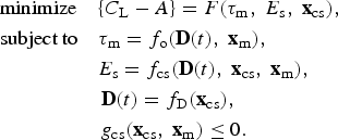 $$\eqalign{& \hbox{minimize}\quad\lcub {C_{\rm L} - A} \rcub {\rm} = F\lpar {{\rm \tau}_{\rm m}\comma \ E_{\rm s}\comma \ {\bf x}_{{\rm cs}}} \rpar\comma \cr & \hbox{subject to}\quad{\rm \tau} _{\rm m} = f_{\rm o} \lpar {{\bf D}\lpar t \rpar\comma\ {\bf x}_{\rm m}} \rpar\comma \cr & \hskip4pc E_{\rm s} = f_{{\rm cs}} \lpar {{\bf D}\lpar t \rpar\comma\ {\bf x}_{{\rm cs}}\comma \ {\bf x}_{\rm m}} \rpar \comma \cr & \hskip4pc \,{\bf D}\lpar t \rpar {\rm} = f_{\rm D} \lpar {{\bf x}_{{\rm cs}}} \rpar\comma \cr & \hskip4pc \,g_{{\rm cs}} \lpar {{\bf x}_{{\rm cs}}\comma \ {\bf x}_{\rm m}} \rpar \le 0.} $$
where C L is the life-cycle cost of the system and A is the availability or other metrics related to availability (such as mean time between maintenance). These are the objectives that need to be minimized and maximized in the design optimization. Life-cycle cost is a common objective for system-level design, and availability is an objective traditionally associated with degradation and maintenance. The objectives are influenced by the variables of τm, E s, and xcs. The vector x consists of all decision variables and, in this problem formulation, is subdivided into the system-level design variables xcs and maintenance variables xm. Examples of system-level design variables can be the types and configuration of components in the system, and examples of maintenance variables include types of maintenance strategies and thresholds for triggering a maintenance event. The τm variable is a sequence of times indicating maintenance occurrences during system life cycle and is computed by the operational subsystem model f o, based on component degradation profiles D(t) and maintenance variables xm. The E s variable is the system-level performance, typically an efficiency or output measure, that is calculated by the physical system models f cs based on degradation profiles, system design variables xcs, and maintenance variables. The component degradation profiles D(t) are generated by degradation subsystem models f D based on system design variables. It is assumed that the degradation profile only describes how the component will degrade over time from its original “clean-state” and thus will only be a function of the system-level design variables. Finally, g cs are the system-level constraints that must be satisfied.
Figure 1 shows the system architecture model associated with this problem formulation. There are two major divisions illustrated in the figure. The first is the system design division that contains the forms and functions of the physical system and its subcomponents and disciplines. The system design model can be highly complicated with many interactions, though in this framework it is generalized into f cs. The second division contains the degradation models f D and the operational model f o, and any other subsystems related to operation. It is assumed that the physical system can be modeled deterministically, while the degradation models are uncertain, and require uncertainty evaluation methods such as Monte Carlo simulation.

Fig. 1. Proposed framework for maintenance integrated at design stage.
The interface between the system design division and the maintenance division can be generalized as follows. The degradation models generate profiles that indicate how each component degrades over time. Multiple components in the system may have degradation profiles that are correlated or independent, and need to be modeled accordingly. These degradation versus time curves are used by the system model f cs to simulate how the system-level performance (E s) will vary over this time period. The performance profiles E s are then fed into the operational model that computes the maintenance pattern τm. The operational model is simulated for N lc years, the total duration of the system life cycle, with different degradation profiles generated over the life cycle to simulate the uncertainty in degradation.
It is critical to model the interdependencies between the subsystem components, and identify the key components and their degradation modes that contribute to system performance losses. System-level modeling techniques such as design structure matrices (Browning, Reference Browning2001; Alfaris et al., Reference Alfaris, Siddiqi, Charbel Rizk and de Weck2010; Eppinger & Browning, Reference Eppinger and Browning2012) and the engineering system matrix (Hu & Cardin, Reference Hu and Cardin2015) can be used for this purpose. Once the key degradation modes are identified, the relationship between degradation and the physical parameters associated with the component needs to be determined. This can be challenging and usually requires expert knowledge specific to the domain of the component. A survey of literature in the field may be an adequate approach to constructing a detailed model of component degradation.
3.2. Objective function definitions
This framework focuses on two design objectives: the life-cycle cost and system availability (time between maintenance). Other objectives may be considered, but cost and availability are representative for comparing optimality of system designs and maintenance strategies. The life-cycle cost C L is defined as the total present cost of the system and contains
 $$C_{\rm L} = C_{\rm C} + C_{\rm M} + C_{\rm E}\comma $$
where C C is the capital cost associated with system development. If any portion of the capital cost occurs later in the system life cycle, then the cost needs to be discounted to the present value with the discount rate r; C M is the maintenance cost, which is the sum of all maintenance costs:
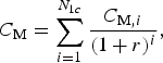 $$C_{\rm M} = \sum\limits_{i = 1}^{N_{1c}} {\displaystyle{{C_{{\rm M}\comma i}} \over {\lpar {1 + r} \rpar ^i}}\comma} $$
and C E is the efficiency cost, which is the cost due to degradation, such as the extra fuel needed:
 $$C_{\rm E} = \sum\limits_{i = 1}^{N_{1c}} {\displaystyle{{C_{{\rm E}\comma i}} \over {\lpar {1 + r} \rpar ^i}}\comma} $$
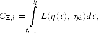 $$C_{{\rm E}\comma i} = \int\limits_{t_{i - 1}} ^{t_i} {L\lpar {{\rm \eta} \lpar {\rm \tau} \rpar\comma\, {\rm \eta}_{\rm d}} \rpar } d{\rm \tau}\comma $$
where η is the actual system efficiency (between time t i−1 and t i), ηd is the designed system efficiency without degradation, and L is a function that computes the monetary loss due to degradation, dependent on the physical system.
The second objective is availability, which is generally defined in the literature as (Stapelberg, Reference Stapelberg2009):
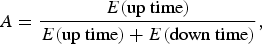 $$A = \displaystyle{{E\lpar {\hbox{up time}} \rpar } \over {E\lpar {\hbox{up time}} \rpar {\rm} + E\lpar {\hbox{down time}} \rpar }}\comma $$
where E() is the expected value operator, up time is the time that the system is operational, and down time is the time the system spent idling, including due to failure and during maintenance. In certain cases, the time taken to perform maintenance may be negligible, then an alternative measurement, mean time between maintenance (MTBM), can be used instead.
In general, the life-cycle cost of the system should be minimized, while the system availability should be maximized. Multiple-objective optimization methods can be used to find the Pareto-optimal designs. Alternatively, one of the two objectives can be treated as an intermediate variable, and single-objective optimization methods can be used.
3.3. Computational complexity
Because there are significant uncertainties associated with the life cycle analysis, uncertainty quantification methods such as Monte Carlo simulation are required to produce many different life cycle simulations to fully characterize the effects of uncertainty. The need for Monte Carlo simulation significantly increases the computational complexity of the framework.
The degradation and maintenance subdivisions of the framework contain all the stochastic models, such as the component degradation models. The physical system model can be assumed to be completely deterministic, and can be treated as a blackbox in the Monte Carlo simulation. The model only needs to be evaluated a few times to generate a surrogate model, such as a look-up table, and the Monte Carlo life cycle simulations can use the surrogate model instead of calling the full system model to reduce computing complexity.
Despite the reduction of computing complexities, the computing requirement is still significant, and thus balancing between model fidelity and complexity is a major challenge. For a multidisciplinary system, domain-specific models are usually high fidelity with very low discrepancies with reality but require significant computational time (on the order of hours or days). Furthermore, high-fidelity discipline-based models are usually represented using different software tools, making the data transfer between models complicated. Thus, high-fidelity models are not the best option for use in this framework. A common approach for model complexity reduction is to generate low-fidelity models from high-fidelity models using metamodeling methods such as Kriging or a response surface method (Wang & Shan, Reference Wang and Shan2007). Low-fidelity models can then be evaluated very quickly, but can have substantial discrepancy.
A midfidelity model is a simplified representation of a system that captures the essence of different domains by using first-order approximations of physics-based models (Lin et al., Reference Lin, de Weck, de Neufville, Robinson and MacGowan2009). Because they are physics based, no special software is needed, and this allows simple integration of different domains and subsystems. A midfidelity model has the advantages of short simulation time on the order of several seconds. Midfidelity models are commonly used in the early design phases to identify promising design strategies. Therefore, it is recommended that midfidelity models be used whenever possible.
3.4. Framework summary
Below are the proposed steps for setting up the integrated design and maintenance optimization problem:
1. Identify key components and their degradation modes that contribute to system performance loss and require regular maintenance services.
2. Determine the relationship between physical parameters and degradation.
3. Propose feasible maintenance strategies. Determine variables associated with maintenance.
4. Construct the system model. Set up domain models for the system, incorporate the degradation relationship, simulate over the lifetime operation of the system, and compute objective functions.
In sum, the proposed modeling framework is an architectural-level modeling approach aimed at capturing the interactions between the design space and the maintenance decision space in a complex engineering system. By identifying and modeling these interactions, designers can explore the trade-offs between different technology, different maintenance strategies, as well as different sets of design parameters. Generally, systems that can benefit from this framework should have the following characteristics: the degradation of key components is stochastic in nature, and the system architecture design choices can significantly affect the development of degradation. Examples include battery systems, membrane-based water production systems, and solar-powered systems.
4. POWER PLANT CONDENSER CASE STUDY
This section illustrates the proposed approach through a case example of designing a condenser heat exchanger in a power system. This system is selected because heat exchangers are widely used in a variety of thermal systems and are subject to constant degradation. The case example will compare different maintenance strategies in the design optimization of the condenser, taking into consideration condenser degradation and maintenance. The purpose of this example problem is to demonstrate the broader implications of the proposed design framework. By modeling degradation and maintenance during the design of system architecture, designers can make more informed decisions by considering the trade-offs between life-cycle cost and availability. Specifically, an advanced maintenance strategy that is based on prognostics of future degradation will result in lower life-cycle cost, and potentially reduce design redundancy.
In a steam power plant, the condenser at the exit of the low-pressure turbine converts the exiting steam into liquid. Condensers are shell-and-tube heat exchangers. The steam flows through the shell side, which is usually kept at a very low pressure to achieve higher cycle efficiency. The heat rejected from the steam condensation is carried away by cooling water in the tube side of the condenser.
Fouling is the major degradation mode of a condenser. Fouling is the buildup of foreign materials inside the tubes due to bioparticles and inorganic salt in the cooling water. Fouling causes high thermal resistance in the condenser (commonly measured as fouling resistance, m2K/kW), which increases the shell side pressure and ultimately reduces plant efficiency. It is recognized as one of the biggest problems associated with efficiency loss in power plants (Taborek et al., Reference Taborek, Aoki, Ritter, Palen and Knudsen1972a).
The buildup of fouling resistance in a condenser usually follows an asymptotic curve (Sheikh et al., Reference Sheikh, Zubair, Younas and Budair2001). The asymptotic values of fouling and the rate of buildup are highly stochastic. Over the past 50 years, much research has focused on finding the underlying physics that governs fouling. The results have suggested that the amount of fouling and the rate of fouling are proportional to temperature, and inversely proportional to the cooling water flow rate, assuming unchanging water quality and tube material (Taborek et al., Reference Taborek, Aoki, Ritter, Palen and Knudsen1972b; Rabas et al., Reference Rabas, Panchal, Sasscer and Schaefer1993).
The maintenance of a condenser is performed offline, commonly during a scheduled power plant outage. Specialized scrapers are shot through the tubes with pressurized water to physically remove built-up foulant. Cleaning can usually be completed within 48 h before returning the condenser to its original condition.
An optimal steam condenser is designed following the proposed framework. Three different maintenance strategies will be considered, and the details of the strategies and the overall system model will be described in detail in the next subsection.
4.1. System modeling
4.1.1. Power model
For simplicity, a Rankine cycle with a single-stage turbine is used. The power cycle only has five components: the boiler, the turbine, the condenser, the cooling water pump, and the feed water pump, as shown in Figure 2.

Fig. 2. Model schematics of Rankine cycle.
To create a numerical model, the Rankine cycle is broken down to six nodes, each representing the steam condition at the inlet and exit of a system component. The nodes are numbered 1 to 6 as shown by the subscripts in Figure 2. The variables P i, Ti, hi, and x i are the pressure, temperature, enthalpy, and steam quality of the fluid at node i, respectively;  ${\dot Q}_{\rm i} $ and
  ${\dot Q}_{\rm o} $ are for the heat (kW) input by the boiler and heat rejected by the condenser;
  ${\dot W}_{\rm t} $,
  ${\dot W}_{{\rm fp}} $, and
  ${\dot W}_{{\rm cp}} $ are the work (kW) extracted through the turbine, input to the feed water pump, and input to the coolant pump, respectively; and
  $\dot m_{\rm s} $ and
  $\dot m_{\rm c} $ are the mass flow rate (kg/s) of the steam/water circulated through the power cycle and cooling water through the condenser.
The power cycle model computes the cycle efficiency η as its output:
 $$\eqalign{& {\rm \eta} = \displaystyle{{\dot W_{\rm o}} \over {\dot Q_i}}\comma} $$
where  ${\dot W}_{\rm o} $ is the net power output of the plant. Losses associated with pipe friction and inefficiency associated with pumps and turbines are neglected. The water/steam properties at each node are defined by the designer (boiler specification: P 3, T 3, turbine back pressure specification: P 4), by the physical environment (T 5), or determined through a steam table (Holmgren, Reference Holmgren2007).
4.1.2. Condenser model
The condenser model computes the condenser heat duty based on the inlet conditions and geometry using the log-mean temperature difference (LMTD) method (Kakac, Reference Kakac1991). The condenser heat load  ${\dot Q}_{\rm c} $ is equal to
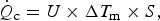 $$\dot Q_{\rm c} = U \times \Delta T_{\rm m} \times S\comma$$
where U is the condenser's overall heat transfer coefficient [W/(m2K)], ΔT m is the LMTD, and S is the overall surface area of the condenser (m2).
It was assumed the condenser is a one-pass X-type shell and tube heat exchanger made of 70–30 copper–nickel alloy, with the terminal conditions listed according to Figure 3, where P atm is the atmospherical pressure, ΔP is the pressure drop in the coolant side of the condenser, and T sat is the saturation temperature of steam at pressure P 4.

Fig. 3. Model schematic of condenser.
An iterative process computes the condenser heat load  ${\dot Q}_{\rm c} $ and coolant pressure loss ΔP based on the condenser geometry (number of tubes Nt and tube length L) and the condenser fouling resistance R f (m2K/W). Details of the model can be found in Kakac (Reference Kakac1991).
4.1.3. Fouling model
Fouling in the condenser is measured by fouling resistance R f. Fouling is a complicated phenomenon that has been studied extensively. A general consensus is that the overall fouling trend can be represented by this asymptotic model (Taborek et al., Reference Taborek, Aoki, Ritter, Palen and Knudsen1972a, Reference Taborek, Aoki, Ritter, Palen and Knudsen1972b; Epstein, Reference Epstein1983; Zubair et al., Reference Zubair, Sheikh, Budair and Badar1997):
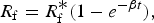 $$R_{\rm f} = R_{\rm f}^{\displaystyle \ast} \lpar {1 - e^{ - {\rm \beta} t}} \rpar\comma $$
where  ${R}_{\rm f}^{\displaystyle \ast} $ is an asymptotic fouling resistance value related to the cooling water velocity v c, tube inner diameter D i, and the kind of foulant, while β (year−1) is the reciprocal of the time constant. Empirical correlations used for
  ${R}_{\rm f}^{\displaystyle \ast} $ with calcium carbonate fouling and β are the following (Caputo et al., Reference Caputo, Pelagagge and Salini2011):
 $$R_{\rm f}^{\displaystyle \ast} = \displaystyle{{0.101} \over {\nu _{\rm c}^{1.33} {D}_{i}^{0.23}}}\comma $$
 $${\rm \beta} = {\rm} 0.0016v_{\rm c} ^{ - 0.35}. $$
 Because fouling is a stochastic process, the asymptotic fouling resistance  $R_{\rm f}^{\displaystyle \ast} $ can change randomly over time (Taborek et al., Reference Taborek, Aoki, Ritter, Palen and Knudsen1972a; Zubair et al., Reference Zubair, Sheikh, Budair and Badar1997). In this study, the asymptotic fouling resistance is considered a random variable (
 ${\bf R}_{\bf F}^{\displaystyle \ast} $) that takes on a new value each time the condenser is cleaned. The distribution of
  ${\bf R}_{\bf F}^{\displaystyle \ast} $ is assumed to be log normal (Taborek et al., Reference Taborek, Aoki, Ritter, Palen and Knudsen1972a):
 $$\eqalign{{\bf R}_{\bf F}^{\displaystyle \ast} &= {\rm LN}\left( {{\rm \mu }\comma\ {\rm \sigma }} \right)\comma\cr {\rm \mu } &= \displaystyle{{0.101} \over {v_{\rm c}^{1.33} D_i^{0.23} }}\comma \cr {\rm \sigma } \big/{\rm \mu } &= 0.3.} $$
4.1.4. Maintenance models
Three types of maintenance strategies are considered: fixed interval, corrective, and predictive. Power plants are usually shut down annually during the spring when energy demand is the lowest. For this study, it is assumed the condenser is inspected and cleaning decisions are made during the annual downtime. A fixed-interval strategy follows a preset schedule to maintain the condenser every N years. Both corrective and predictive strategies are based on monitoring the fouling resistance and comparing to a threshold value R fs. In corrective maintenance, cleaning happens if current R f> R fs. In preventive maintenance, a RUL is estimated each year by predicting when R f will exceed R fs, and schedule cleaning if RUL < 1 year. In this study, the prediction algorithm is assumed to be perfect.
4.1.5. Operation and economics model
A 50-year lifetime is assumed for the power plant. The life-cycle cost C L consists of the capital cost C C, maintenance cost C M, and efficiency cost C E as indicated previously in Eq. (2).
For simplicity, only the capital cost of the condenser is considered for this study, which is proportional to the amount of materials used in the condenser tubes.
 $$C_{\rm C} = {\bf P}_{\bf m} {\rm \rho} _{\rm m} N_{\rm t} L\displaystyle{{\rm \pi} \over 4}(D_{\rm o}^2 - D_i^2 )\comma$$
where Pm is the price of raw material ($/kg), ρm is the density of material (kg/m3), and  ${N}_{\rm t} {L}\lpar{{\rm \pi} / \hbox{4}}\rpar \lpar {{D}_{\rm o}^{\rm 2} - {D}_{i}^{\rm 2}} \rpar $ is the total material volume of the condenser tubes. Capital cost associated with implementing maintenance strategies, such as sensors and computing equipment, are not considered in this study for simplicity.
The maintenance cost is associated with the physical cleaning of the condenser tubes. The annual cleaning cost C M,i is either zero when there is no cleaning during the year or
 $$C_{{\rm M}\comma i} = {\bf P}_{\bf L} + {\bf P}_{\bf s} N_{\rm t}\comma $$
when cleaning is performed. The first part is the fixed maintenance cost where PL is the cost of labor, and the second part is the cleaning equipment cost and depends on how many tubes are in the condenser, and Ps, which is the price of each scraper.
The efficiency cost is an estimate of the productivity lost due to fouling. It was assumed the plant has zero efficiency cost when it operates at the designed efficiency ηd, which is the Rankine cycle efficiency if fouling resistance is zero. Efficiency cost increases proportionally to the amount of extra fuel consumed as a result of fouling. The annual efficiency cost C E,i is computed as
 $$C_{{\rm E}\comma i} = \displaystyle{{{\bf P}_{\bf f}} \over {\hbox{HV}}}\int\limits_{t_{i - 1}} ^{t_i} {W_{\rm o} \lpar {\rm \tau} \rpar \left( {\displaystyle{1 \over {{\rm \eta} \lpar {\rm \tau} \rpar }} - \displaystyle{1 \over {{\rm \eta}_{\rm d}}}} \right)d{\rm \tau}\comma} $$
where Pf is the price of fuel ($/kg), HV is the heating value of the fuel (kJ/kg), W o is the actual instantaneous power output during the year i, and η is the actual instantaneous thermal efficiency during the year i.
The annual maintenance cost C M,i and efficiency cost C E,i are discounted to present value using a discount rate r to obtain C M and C E, according to Eqs. (3) and (4).
4.1.6. Model integration
According to the proposed modeling structure, the system model is divided into a deterministic model, which includes the power and condenser models, and a probabilistic model, which includes the fouling and operation models.
For simplicity, boiler temperature and pressure are kept as constant parameters, and the only design variables considered are the number of condenser tubes N t and the condenser tube length L. Constraints in the power-condenser model include the minimum turbine back pressure P 4,l and the maximum condenser coolant flow rate  $\dot m_{{\rm c}\comma l} $. The deterministic system model has an input–output relationship of
 $${\rm \eta} = f_{{\rm sys}} \lpar {N_{\rm t}\comma\ L\comma \ R_{{\rm fs}}} \rpar .$$
In the probabilistic subsystem models, the operational model uses a Monte Carlo simulation to simulate the life cycle of the power plant randomly multiple times. The simulation process is shown in the flow chart in Figure 4.
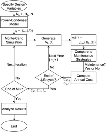
Fig. 4. Model evaluation process.
At the beginning of the simulation, system-level design parameters are specified to determine the physical design of the condenser, and then a Monte Carlo simulation is performed to evaluate the performance of the system. Each iteration of the Monte Carlo simulation generates a life cycle simulation of the plant. At the beginning of the plant's life cycle, a fouling profile R f,j(t) is generated with the asymptotic fouling resistance  $R_{\rm f}^{\displaystyle \ast} $ randomly generated from the log-normal distribution described in Eq. (12). The operation model simulates the plant operation on a year-to-year basis and determines when maintenance is needed. After the occurrence of each maintenance event, the condenser is assumed to return to its original clean condition, and a new asymptotic fouling resistance is generated. After the entire life cycle is completed, a new life cycle is generated by the Monte Carlo simulation, and this process repeats until the desired number of iterations is reached. In this example, the Monte Carlo iteration number was set to 1000.
Some designer-defined parameter values used in the modeling process are tabulated in Table 1. The condenser cleaning equipment and labor costs are obtained from CONCO Systems, a manufacturer of heat exchanger cleaning equipment. Fuel cost is estimated based on the price of clean coal provided by the US Energy Information Administration, and the cost of condenser tube material is the average quoted price of several online vendors.
Table 1. List of user-defined parameters

4.2. Traditional design method (LMTD method)
Traditionally, the LMTD design process of choosing a condenser is based on the following three-step process (Kakac, Reference Kakac1991):
1. Determine the condenser heat load
 $\dot Q_{\rm c} $ from the power plant's requirements.
2. Select an operating fouling resistance based on empirical correlations.
3. Determine the overall heat transfer coefficient U, the LMTD, and consequently calculate the condenser area, from which L and N t are determined.

The process is similar to adding design redundancy into the condenser. The fouling resistances for different fluids are tabulated in heat exchanger design handbooks. For example, the Tubular Exchanger Manufacturers Association lists fouling resistances for seawater to be 0.352 m2K/kW and for brackish water to be 0.176 m2K/kW.
Once the fouling resistance is selected, the condenser design variables, N t and L, can be determined using the LMTD method. For this case example, the fouling resistance was chosen to be 0.3 m2K/kW, in between the values of seawater and brackish water, and found that using the traditional design method, the condenser would require 7280 tubes and a tube length of 14.7 m.
Based on this specific condenser design, the three different maintenance strategies can be analyzed independently by simulating the life cycle with uncertainties, and a simple maintenance optimization can be solved to find the most optimal maintenance variable that results in the minimum life-cycle cost (C L) of the system. The problem definition is shown below:
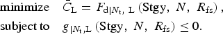 $$\eqalign{&{\rm minimize}\quad{\bar C}_{\rm L} = F_{{\rm d}{\vert N_{\rm t}\comma\ {\rm L}}} \left( {{\rm Stgy}\comma\ N\comma \ R_{{\rm fs}}} \right)\comma \cr & {\rm subject}\,{\rm to}\quad g_{\vert N_{\rm t}\comma {\rm L}}\left( {{\rm Stgy}\comma \ N\comma \ R_{{\rm fs}}} \right) \le 0.} $$
where  ${\rm \bar C}_{\rm L} $ is the mean value of the life-cycle cost from the Monte Carlo system model simulation, Stgy indicates one of the three maintenance strategies being considered: fixed interval, for which N is the maintenance interval in number of years, corrective and preventive, for which R fs is the fouling resistance threshold, and F d and g are the system models described in the section above.
The problem formulation is a mixed-integer nonlinear programming problem. However, because only three different strategies are being considered, they can be analyzed independently, and the other integer variable N is only associated with the fixed-interval strategy and can be handled through an exhaustive search, and thus reduces the problem down to a set of continuous nonlinear problems.
4.3. Optimal design method
The proposed framework allows an optimal condenser design to be found directly through optimization of the full system model. The problem definition is
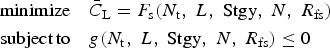 $$\eqalign{& \hbox{minimize}\quad\bar C_{\rm L} = F_{\rm s} \lpar {N_{\rm t}\comma\ L\comma \ \hbox{Stgy}\comma \ N\comma \ R_{{\rm fs}}} \rpar \cr & \hbox{subject}\,\hbox{to}\quad g\lpar {N_{\rm t}\comma \ L\comma\ \hbox{Stgy}\comma\ N\comma \ R_{{\rm fs}}} \rpar \le 0} $$
Similar to the maintenance optimization problem described in the previous section, this mixed-integer nonlinear programming problem can also be reduced into several continuous nonlinear problems by independently analyzing the three different maintenance strategies.
All of the programming and simulation for this case example were done in MATLAB 2011a. Built-in optimization algorithms including “ga” (genetic algorithm) were used. Because the Monte Carlo simulation resulted in long function evaluations, a population size of 30 with 20 generations were used to limit the overall computing time. In addition, “fmincon” (sequential quadratic programming) with random initial starting points was also used, and provided results with values within 2% of the genetic algorithm.
5. RESULTS
This section describes the results from the case study detailed above to demonstrate the proposed design–maintenance optimization framework, and how it can be used to improve designer's understanding of trade-offs between different subsystems and disciplines. Comparisons between traditional and optimal design methods, and between different maintenance strategies, were made. It is expected that considering maintenance strategies during system architecture design would improve the system-level performance in both life-cycle cost and availability.
5.1. Single-objective optimization
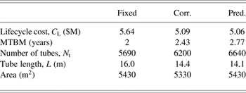
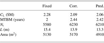
The maintenance optimization problem for the traditional design approach described in Eq. (17) and the optimal design problem described in Eq. (18) were both solved. The design that resulted in the lowest life-cycle cost was found, and MTBM for each design is also computed, which is a measure of the availability of the system. The life-cycle cost and MTBM for each maintenance strategy and the two different design approaches are given in Table 2.
Table 2. Results of traditional design versus optimal design

Comparing the three different maintenance strategies, the fixed-interval strategy resulted in the highest life-cycle cost, and also lowest MTBM (lowest availability). Using maintenance strategies based on fouling-monitoring (corrective and predictive) reduced life-cycle cost, and also extended MTBM (higher availability). This is to be expected because the fixed-interval strategy ignores any uncertainty associated with degradation, while fouling-monitoring based strategies adapt the maintenance schedule to the actual fouling trend. A preventive maintenance strategy results in slightly lower cost and longer MTBM compared to corrective maintenance, because the predictive capability allows an operation to be cut short if the fouling resistance develops rapidly, while it still allow long periods of operation if fouling development is minimal.
Comparing traditional and optimal approaches to the condenser design, the optimal design approach reduces the total life-cycle cost significantly for the fixed-interval maintenance case, while cost reductions in the corrective and preventive maintenance cases are not as significant. However, the MTBM is improved significantly.
Figure 5 shows the break down of the life-cycle cost into capital, cleaning, and efficiency costs. In the traditional design approach, the capital costs for all three strategies are the same, because the same condenser design is considered. The fixed-interval strategy, however, has significantly higher cleaning cost and efficiency cost, while the efficiency costs between corrective and predictive maintenance are similar, and predictive maintenance has a lower cleaning cost, because the longer MTBM value results in fewer maintenance operations.

Fig. 5. Life cycle cost breakdown, traditional design versus optimal design.
With the optimal design approach, cleaning cost is reduced for all three maintenance strategies by using a condenser with fewer tubes as shown in Table 3. Optimization with a fixed-interval strategy resulted in significant cost reductions, but the overall cost is still more than designs with monitoring-based maintenance methods. It is interesting to note that the optimal design with corrective maintenance had similar cleaning and efficiency costs compared to the design with predictive maintenance, but the capital cost was higher for design with corrective maintenance because a larger condenser was needed (longer tubes and higher area, shown in Table 3). This is consistent with results found in similar studies, indicating design redundancy can be replaced by advanced maintenance strategies (Bodden et al., Reference Bodden, Hadden, Grube and Clements2005; Youn et al., Reference Youn, Hu and Wang2011). By implementing the proposed framework, the designers can now consider parameters and decisions that do not directly relate to fouling, but are coupled with fouling and maintenance on a system level.
Table 3. Results of optimal condenser design

It should be noted that the capital cost associated with implementing the maintenance infrastructure (sensors and computing equipment) is neglected, because the cost will vary based on the type of maintenance and, in the case of predictive maintenance, the accuracy of the prediction. Incorporating the infrastructure cost will have the effect of changing the trade-offs between life-cycle cost and availability.
5.2. Parameter sensitivity
A large number of design parameters are involved in the modeling process; thus, understanding how the optimal design changes when the parameter values are changed is a critical step in the design optimization process. In this section, the optimal design approach was reevaluated under different parameter values, to compare to the optimal design found with the default parameter values.
5.2.1. Condenser cost
To assess the sensitivity of the model to condenser cost, the cost of condenser tubes is increased from the default value of $20/kg to $40/kg, and optimization analysis is performed again to find the optimal condenser design with the new parameter value. The results are shown in Table 4, and shows that the total life-cycle costs increased roughly 25% from the default parameter values, the MTBM values were lower compared to the default designs, and the condenser area is smaller compared to the default designs.
Table 4. Optimal condenser design: 2× condenser cost
The increase in condenser capital cost resulted in the optimization algorithm picking a smaller condenser and reduces the average cleaning interval to compensate for the smaller condenser (Fig. 6). The advantage of predictive maintenance over corrective maintenance appears to increase, because the MTBM value for the design with predictive maintenance is noticeably longer than corrective maintenance.

Fig. 6. Life-cycle cost breakdown: 2 × condenser cost.
5.2.2. Discount rate
In the default analysis, no discount rate was considered, and costs incurred anytime during the system life cycle were considered the same. Table 5 shows the condenser design found by the optimization algorithm with a discount rate of r = 5% applied to the model (Fig. 7). As expected, the net present life-cycle cost decreased significantly, especially the cleaning and efficiency cost, due to discounting of costs over the life cycle.
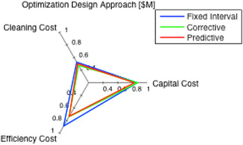
Fig. 7. Life-cycle cost breakdown: r = 0.05.
Table 5. Optimal condenser design: discount rate r = 0.05
Three effects are noticeable when the discount rate is considered compared to the default case. The MTBM values for designs with corrective and predictive maintenance decrease from ~3 to ~2.4 years, the capital cost decreases from $1M to about $0.8M, and the optimal condenser is smaller with area in the 5000 m2 range, compared to the 6000 m2 range for the default. It is also observed that corrective and predictive maintenance are now almost equally effective, with similar life-cycle costs and MTBM values. This result was surprising but reasonable. The discounting makes the cost of maintenance and lost efficiency lower compared to the capital cost, and the major advantage of predictive maintenance is in reducing unnecessary maintenance while keeping efficiency high.
5.2.3. Implication of sensitivity analysis
The sensitivity analyses suggest that, with different values of system parameters, such as cost of material and discount rate, the trade-off relationship between life-cycle cost and availability will change to reflect the optimal design solution under the new set of system parameters. By varying the model parameter values, designers can gain insights into how maintenance strategies and design variables interact, and some of the interactions may not be obvious. This system-level approach of modeling physical design and maintenance operations concurrently has the ability to reveal these nonobvious insights about the system. Similar studies can be performed on other parameters and variables of the model to obtain additional information.
5.3. Multiple-objective optimization
Multiple-objective optimization was performed to find the Pareto-optimal designs that minimizes life-cycle cost and maximizes MTBM. The problem formulation is described as follows:
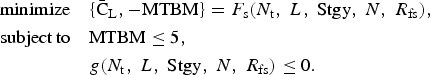 $$\eqalign{& \hbox{minimize}\quad\lcub {{\rm \bar C}_{\rm L}\comma - \hbox{MTBM}} \rcub = F_{\rm s} \lpar {N_{\rm t}\comma \ L\comma \ \hbox{Stgy}\comma\ N\comma \ R_{{\rm fs}}} \rpar\comma \cr & \hbox{subject}\,\hbox{to}\quad\hbox{MTBM} \le 5\comma \cr & \hskip4pc g\lpar {N_{\rm t}\comma \ L\comma\ \hbox{Stgy}\comma\ N\comma \ R_{{\rm fs}}} \rpar \le 0.} $$
The maximum MTBM value is artificially limited to 5 years for this study. MATLAB built-in multiobjective genetic algorithm “gamultiobj” was used.
Figure 8 shows the Pareto fronts for the optimization results with corrective maintenance and predictive maintenance. Fixed-interval maintenance results are significantly higher (by over $1M) compared to the corrective and predictive strategies and are not shown in the figure. The predictive maintenance designs completely dominate the corrective maintenance designs. It is interesting to note that the Pareto front for predictive strategy is very similar in shape to the corrective strategy: one is simply a shifted version of another, and the predictive strategy results in longer MTBM and lower cost. Although not shown here, the fixed-interval strategy produced a completely different-shaped Pareto front: life-cycle cost equal to $5.6M at MTBM equal to 2 years, and increasing almost linearly to $7.6M, at MTBM equal to 5 years. This suggests that predictive and corrective strategies are better at handling systems requiring long MTBM values.

Fig. 8. Results of multiple-objective optimization.
It should be noted that the Pareto fronts generated through multiobjective genetic algorithms are not the analytical Pareto fronts, and the shapes of the fronts are sensitive to model parameter variations. Despite these shortcomings, the Pareto fronts cans still provide valuable insights for the designers when making decisions on selecting a maintenance strategy.
6. CONCLUSIONS AND FUTURE WORK
This study presents a framework for integrating maintenance during system architecture design in order to capture and predict the relationships between system-level component design and maintenance planning. The proposed approach addressed the challenge of suboptimal life-cycle performance due to the uncertainties and interdependencies associated with operation and maintenance of engineering systems. A case example of a condenser design was used to demonstrate the significance of different maintenance strategies and their effects on system design decisions. Three maintenance policies were considered: fixed maintenance interval, corrective maintenance based on degradation threshold, and predictive maintenance based on the prediction of future degradation. Single-objective optimization, sensitivity analyses, and multiobjective optimization were conducted on the case study, and the outcomes of the example design problem show that by concurrently optimizing both the system design variables and the maintenance variables, both the life-cycle cost and the overall availability of the system can be improved compared to sequentially optimizing system-level design and maintenance decisions. The optimal design will also change with different maintenance policies, which is not obvious in the traditional sequential design approach. This information provided by the proposed approach can help designers in the early design stage to select the optimal system architecture that captures the effect of maintenance during the operation of the system.
Two major assumptions were made in this work to simplify the analysis. First, the costs associated with implementing different maintenance strategies are neglected. In reality, there would be additional capital and operational costs associated with the necessary sensors for degradation monitoring, and computing equipment for making degradation predictions. However, the life-cycle cost analysis presented here can still reveal valuable information about the different maintenance strategies, and can help designers decide whether the benefits from advanced maintenance strategies can justify their added costs. Second, the other major assumption is that the algorithm used in predictive maintenance can perfectly predict the future. Any uncertainties associated with the prediction algorithm would reduce the advantages of predictive maintenance observed in this study. Future research should consider simulations with different values of prediction uncertainties to understand their effects.
The proposed framework takes a system-level approach by integrating the maintenance strategies and life cycle analysis with the design process, and thus significantly increased the problem complexity. Efforts to reduce complexity included decoupling the uncertain degradation and maintenance models from the deterministic system models, and implementing midfidelity physics-based models. Future research efforts should look into the effects of having multiple degrading components.
The example presented in this paper focused on helping designers evaluate the trade-offs between different maintenance strategies and design parameter values. It is the intent that this approach can be straightforwardly extended to explore more complex system architecture designs. An example of this might be the interactions between different design choices, such as desalination technologies (membrane vs. distillation), and different energy sources. Future study should also focus on exploring the design–maintenance space by including the different uncertain parameters, such as energy and resource pricing, to evaluate the sensitivity of a design to maintenance policy.
ACKNOWLEDGMENTS
We thank the King Fahd University of Petroleum and Minerals for funding the research reported in this paper through the Center for Clean Water and Clean Energy at the Massachusetts Institute of Technology and the King Fahd University of Petroleum and Minerals under Project R13-CW-10. This work also received partial support from the National Science and Engineering Council of Canada. The opinions, findings, conclusions, and recommendations expressed are those of the authors and do not necessarily reflect the views of the sponsors.
Bo Yang Yu is a Postdoctoral Associate at the Massachusetts Institute of Technology. He received his BS and MS in mechanical and mechatronics engineering from the University of Waterloo in Canada and his PhD degree in mechanical engineering from the Massachusetts Institute of Technology. Dr. Yu is a member of ASME and the recipient of a National Science and Engineering Research Council of Canada postgraduate award.
Tomonori Honda is currently Senior Data Scientist at 4INFO and Visiting Research Scientist at the Massachusetts Institute of Technology. He received his PhD and MS in mechanical engineering from the California Institute of Technology and BS in mechanical engineering and nuclear engineering from the University of California, Berkeley. Dr. Honda is member of ASME, AIAA, and AAAI and has reviewed papers for many journals. His main research areas include data-driven modeling for industrial applications; design for system reliability, prognosis, and maintenance; design synthesis for complex systems; and behavioral design theory.
Syed Zubair is a Distinguished Professor in the Mechanical Engineering Department at King Fahd University of Petroleum and Minerals (KFUPM). He earned his PhD degree from Georgia Institute of Technology. He is active in both teaching and research in the area of design, performance evaluation, and improvement of thermal systems. He has participated in several externally and internally funded research projects at KFUPM and has published over 200 research papers. Dr. Zubair received the Distinguished Researcher award from the university in academic years 1993–1994, 1997–1998, and 2005–2006 as well as the Distinguished Teacher award in academic years 1992–1993 and 2002–2003.
Mostafa H. Sharqawy is an Assistant Professor of mechanical engineering at the University of Guelph. He is a licensed Professional Engineer in Ontario and a member of ASME and IDA. He worked on many research projects at the University of Tennessee, Massachusetts Institute of Technology, King Fahd University of Petroleum and Minerals, Arizona State University, and University of Guelph. He published more than 60 papers in engineering and scientific-refereed journals and international conference proceedings and holds eight US patents that have been commercialized in the energy industry. In addition, he previously served as an aquatic designer at OLC Corporation in Denver, Colorado. His primary research focus is in the area of sustainable energy and water systems.
Maria C. Yang is an Associate Professor of mechanical engineering at the Massachusetts Institute of Technology. She earned her SB from the Massachusetts Institute of Technology and her MS and PhD from Stanford University, all in mechanical engineering. Dr. Yang previously served as Director of Design at Reactivity, a Silicon Valley start-up now a part of Cisco Systems. She is a Fellow of the American Society of Mechanical Engineers and is a recipient of the National Science Foundation Faculty Early Career award and the American Society for Engineering Educations Merryfield Design Award. Her research centers on the preliminary phases of the process of designing both products and complex engineering systems.


