


1 Introduction
In this paper we investigate the effects of a steady, surface trapped background current
 $\bar{U}(z)$
on the two-dimensional generation of oceanic internal waves by tidal currents oscillating over a symmetric ridge in the weakly nonlinear regime. Figure 1(a) shows the wave-induced horizontal currents after 15 tidal periods from a fully nonlinear numerical simulation (details of the simulations are provided in § 2). The background current lies above
$\bar{U}(z)$
on the two-dimensional generation of oceanic internal waves by tidal currents oscillating over a symmetric ridge in the weakly nonlinear regime. Figure 1(a) shows the wave-induced horizontal currents after 15 tidal periods from a fully nonlinear numerical simulation (details of the simulations are provided in § 2). The background current lies above
 $z/H=-0.3$
,
$z/H=-0.3$
,
 $z$
and
$z$
and
 $H$
being the vertical coordinate and deep water depth respectively, and is directed to the right. Obvious asymmetries in the wave field are apparent. Mode-one waves have propagated outside the region shown. Mode-two waves have reached
$H$
being the vertical coordinate and deep water depth respectively, and is directed to the right. Obvious asymmetries in the wave field are apparent. Mode-one waves have propagated outside the region shown. Mode-two waves have reached
 $x/H\approx -80$
and
$x/H\approx -80$
and
 $120$
in the upstream and downstream directions. Internal wave beams are much stronger in the upstream direction and there is a fan-like structure near the surface downstream of the ridge (
$120$
in the upstream and downstream directions. Internal wave beams are much stronger in the upstream direction and there is a fan-like structure near the surface downstream of the ridge (
 $x/H$
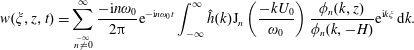
between 0 and 80). Figure 1(b) shows the wave-induced horizontal baroclinic currents predicted by linear theory (§ 4) in which the contributions for each mode are restricted to lie within the distance they would propagate in 15 tidal periods at their group velocity. The theory predicts the wave field quite well although there are differences. Figure 1(c) compares the simulated and theoretical wave-induced surface currents showing excellent agreement.
$x/H$
between 0 and 80). Figure 1(b) shows the wave-induced horizontal baroclinic currents predicted by linear theory (§ 4) in which the contributions for each mode are restricted to lie within the distance they would propagate in 15 tidal periods at their group velocity. The theory predicts the wave field quite well although there are differences. Figure 1(c) compares the simulated and theoretical wave-induced surface currents showing excellent agreement.
Upstream of the ridge the wavelength of the beams is approximately 11.4 versus the mode-one wavelength of 12.5. The strong horizontal currents where the beam reaches the surface are clearly detectable in figure 1(c). Because the wavelengths of the different modes are non-commensurable due to the background current, the internal wave beams that form lose their coherence with distance from the ridge. This also explains the difference in beam wavelength from the mode-one wavelength.

Figure 1. Comparison of wave-induced dimensionless horizontal current fields
 $U/(NH)$
at
$U/(NH)$
at
 $t=15T$
from a numerical simulation (a) and theory (b). Here
$t=15T$
from a numerical simulation (a) and theory (b). Here
 $N$
is the constant buoyancy frequency and
$N$
is the constant buoyancy frequency and
 $H$
the deep water depth. Panel (c) compares the wave-induced horizontal currents at the surface (black, simulation; red, theory). Narrowest ridge from set 4 (see table 1):
$H$
the deep water depth. Panel (c) compares the wave-induced horizontal currents at the surface (black, simulation; red, theory). Narrowest ridge from set 4 (see table 1):
 $h_{0}/H=0.1$
,
$h_{0}/H=0.1$
,
 $a/H=1.2$
,
$a/H=1.2$
,
 $(U_{s}/(NH),z_{s}/H,d_{s}/H)=(0.1,-0.3,0.08)$
.
$(U_{s}/(NH),z_{s}/H,d_{s}/H)=(0.1,-0.3,0.08)$
.
Figure 2 shows the mean wave-induced horizontal currents for a slightly wider ridge. The structure of the mean currents upstream and downstream of the ridge are very different. The quasi-periodic pattern upstream (left) of the ridge is reflected in the energy flux contributions (see § 6). The mean current upstream of the ridge is large at the surface, where it is always positive, at the base of the shear layer, and where beams reflect off the bottom. At the base of the shear layer there are alternating patches of positive and negative mean currents with the latter higher up than the former. This is consistent with beams reaching the base of the current and exerting a stress which raises the base of the current slightly, hence reducing the mean current, and lowering the base of the current slightly between the beams, hence increasing the mean current. To the left of the ridge the maximum and minimum mean currents are approximately
 $10^{-4}$
, approximately a factor of 50 less than the currents associated with the waves of tidal frequency (see figure 1). In dimensional terms they are approximately
$10^{-4}$
, approximately a factor of 50 less than the currents associated with the waves of tidal frequency (see figure 1). In dimensional terms they are approximately
 $0.4~\text{mm}~\text{s}^{-1}$
. Downstream of the ridge the mean currents are about twice as strong.
$0.4~\text{mm}~\text{s}^{-1}$
. Downstream of the ridge the mean currents are about twice as strong.
Figures 1 and 2 show significant asymmetries in the wave field upstream and downstream of the ridge. Associated with this are asymmetries in the energy fluxes which is the primary focus of this paper. Somewhat surprisingly, in the parameter regime we consider, for wide ridges the upstream energy flux is smaller than the downstream energy flux while the opposite is the case for narrow ridges. In the presence of a strong background current the kinetic energy flux makes an important contribution to the total flux and fluxes associated with the mean wave-induced fields are also significant.

Figure 2. Mean horizontal velocity perturbation (dimensionless). Similar case to that depicted in figure 1 (slightly wider ridge from set 4 with
 $a/H=1.8$
: see table 1). Averaging done over
$a/H=1.8$
: see table 1). Averaging done over
 $t\in [36T,40T]$
, where
$t\in [36T,40T]$
, where
 $T$
is the tidal period, in a Lagrangian reference frame moving with the barotropic tidal currents. Green–blue colours are negative currents, red–orange are positive currents. Contour interval
$T$
is the tidal period, in a Lagrangian reference frame moving with the barotropic tidal currents. Green–blue colours are negative currents, red–orange are positive currents. Contour interval
 $10^{-5}$
.
$10^{-5}$
.
Internal wave generation by tide–topography interactions has received a lot of attention over the past couple of decades. This process is estimated to transfer energy from the barotropic tide to internal tides at a rate of approximately 1 TW and accounts for approximately 25 %–30 % of the barotropic tidal energy dissipation (Egbert & Ray Reference Egbert and Ray2001; Nikurashin & Ferrari Reference Nikurashin and Ferrari2013; Waterhouse et al. Reference Waterhouse, MacKinnon, Nash, Alford, Kunze, Simmons, Polzin, St. Laurent, Sun and Pinkel2014). It is also the source of approximately 50 % of the internal wave energy in the ocean, approximately of equal importance to wind forcing. Accurate modelling or parametrizations of this process are necessary for modelling global barotropic tides (Lyard et al. Reference Lyard, Lefevre, Letellier and Francis2006; Buijsman et al. Reference Buijsman, Ansong, Arbic, Richman, Shriver, Timko, Wallcraft, Whalen and Zhao2016) and for taking proper account of mixing by internal waves which is believed to be essential for the large scale overturning circulation in the ocean (Munk & Wunsch Reference Munk and Wunsch1998; Wunsch & Ferrari Reference Wunsch and Ferrari2004; Nikurashin & Ferrari Reference Nikurashin and Ferrari2013). Energy transferred to the internal wave field is partly dissipated near the bottom above rough topography (Polzin et al. Reference Polzin, Toole, Ledwell and Schmitt1997; Waterhouse et al. Reference Waterhouse, MacKinnon, Nash, Alford, Kunze, Simmons, Polzin, St. Laurent, Sun and Pinkel2014; Lefauve, Muller & Melet Reference Lefauve, Muller and Melet2015; Ferrari et al. Reference Ferrari, Mashayek, McDougall, Nikurashin and Campin2016) but can propagate large distances before dissipating when the waves are primarily generated by isolated bathymetric features (Falahat et al. Reference Falahat, Nycander, Roquet, Thurnherr and Hibiya2014). Internal tide generation in the deep ocean was reviewed by Garrett & Kunze (Reference Garrett and Kunze2007).
Geostrophic currents also interact with bathymetry to generate internal lee waves injecting approximately 0.2–0.4 TW into the internal wave field (Scott et al. Reference Scott, Goff, Naveira Garabato and Nurser2011; Nikurashin & Ferrari Reference Nikurashin and Ferrari2013) predominantly in the Southern Ocean where the interaction of the Antarctic Circumpolar Current with bathymetry is an important generator of internal waves.
Considering the ubiquitous presence of large scale currents and eddies in the ocean many tide–topography interactions will inevitably involve background currents although there have been few studies of this process. Pickering et al. (Reference Pickering, Alford, Nash, Rainville, Buijsman, Ko and Lim2015) considered the effects of mean flows on wave generation and energy fluxes in Luzon Strait during periods when the Kuroshio Current passes through the strait. The focus of their study was on energy fluxes at the generation site, not on energy fluxes in the far field. The Indonesian Throughflow passing through Lombok Strait (Aiki, Matthews & Lamb Reference Aiki, Matthews and Lamb2011; Matthews et al. Reference Matthews, Aiki, Masuda, Awaji and Ishikawa2011) and the South Equatorial Current passing over the Mascarene Plateau (da Silva, New & Magalhaes Reference da Silva, New and Magalhaes2011) have been shown to affect the generation of internal solitary waves. Another example includes exchange flows through the Straits of Gibraltar. All of these examples involve large sills which interact directly with the currents.
The effects of a mean flow over ridge-like topography on internal wave generation by tide–topography interactions have not, to our knowledge, been previously considered in numerical or theoretical studies. Here we address this lack by considering the effects of a background current
 $\bar{U}(z)$
confined to a surface layer lying well above the ridge so that there is no direct interaction between the current and the bathymetry which would result in the co-generation of lee waves. We conduct numerical simulations using a fully nonlinear two-dimensional model. For simplicity our background currents satisfy
$\bar{U}(z)$
confined to a surface layer lying well above the ridge so that there is no direct interaction between the current and the bathymetry which would result in the co-generation of lee waves. We conduct numerical simulations using a fully nonlinear two-dimensional model. For simplicity our background currents satisfy
 $\bar{U}(z)\geqslant 0$
and a linear stratification is used.
$\bar{U}(z)\geqslant 0$
and a linear stratification is used.
A linear theory is also developed to predict the internal waves generated by the tide–topography interactions. Our theory is an extension of that presented by Bell (Reference Bell1975a ,Reference Bell b ) and Khatiwala (Reference Khatiwala2003). Bell (Reference Bell1975b ) considered an infinitely deep ocean predicting the vertically propagating internal waves generated by weak oscillating currents over a small subcritical isolated topographic feature. Khatiwala (Reference Khatiwala2003) extended this method to a finite depth ocean with a linear stratification. We extend his method to an arbitrary stably stratified shear flow with the restriction that the current lies above the bathymetry. One cost of this extension is that fewer results can be computed analytically. The theory is valid for small amplitude, subcritical bathymetry and small tidal excursion distances. Neither the theory nor the numerical simulations include the effects of rotation as this would require a transverse pressure gradient in geostrophic balance with the background current. While rotation could be included in the numerical simulations, it implies a density field that varies in the cross-current direction, making the problem three-dimensional.
Section 2 describes the numerical model and the simulations. Energy flux, as calculated in the nonlinear, non-hydrostatic numerical simulations, is discussed in § 3 and the linear theory is developed in § 4. Results of convergence and validation tests are given in § 5 while the main results are presented in § 6 followed by the conclusions and summary in § 7.
2 Numerical model and model set-up
We use the two-dimensional non-hydrostatic Internal Gravity Wave model (Lamb Reference Lamb1994, Reference Lamb2007) to solve the incompressible Euler equations under the Boussinesq approximation in a non-rotating reference frame. The model equations are
 $$\begin{eqnarray}\displaystyle & \displaystyle u_{t}+uu_{x}+wu_{z}=-p_{x}, & \displaystyle\end{eqnarray}$$
 $$\begin{eqnarray}\displaystyle & \displaystyle w_{t}+uw_{x}+ww_{z}=-p_{z}-\unicode[STIX]{x1D70C}g, & \displaystyle\end{eqnarray}$$
 $$\begin{eqnarray}\displaystyle & \displaystyle \unicode[STIX]{x1D70C}_{t}+u\unicode[STIX]{x1D70C}_{x}+w\unicode[STIX]{x1D70C}_{z}=0, & \displaystyle\end{eqnarray}$$
 $$\begin{eqnarray}\displaystyle & \displaystyle \unicode[STIX]{x1D735}\boldsymbol{\cdot }\boldsymbol{u}=0. & \displaystyle\end{eqnarray}$$
 $\boldsymbol{u}=(u,w)$
is the velocity in the vertical
$\boldsymbol{u}=(u,w)$
is the velocity in the vertical
 $xz$
-plane,
$xz$
-plane,
 $\unicode[STIX]{x1D70C}$
is the density and
$\unicode[STIX]{x1D70C}$
is the density and
 $p$
is the pressure, both of which have been scaled by the reference density
$p$
is the pressure, both of which have been scaled by the reference density
 $\unicode[STIX]{x1D70C}_{0}$
. The rigid lid approximation is used with the surface at
$\unicode[STIX]{x1D70C}_{0}$
. The rigid lid approximation is used with the surface at
 $z=0$
. We consider waves generated by tidal flow over an isolated topographic feature at
$z=0$
. We consider waves generated by tidal flow over an isolated topographic feature at
 $z=-H+h(x)$
such that
$z=-H+h(x)$
such that
 $h(x)\rightarrow 0$
as
$h(x)\rightarrow 0$
as
 $x\rightarrow \pm \infty$
. The model uses Godunov flux limiting which acts as an implicit large eddy simulation model (Bell, Colella & Glaz Reference Bell, Colella and Glaz1989). Terrain following coordinates are used which leads to higher vertical resolution in shallower water. In these simulations the time step is fixed.
$x\rightarrow \pm \infty$
. The model uses Godunov flux limiting which acts as an implicit large eddy simulation model (Bell, Colella & Glaz Reference Bell, Colella and Glaz1989). Terrain following coordinates are used which leads to higher vertical resolution in shallower water. In these simulations the time step is fixed.
Figure 3 shows a schematic of the numerical set-up. The simulations were conducted using dimensional variables with the deep ocean in mind. We used a fluid of depth
 $H=5000$
m in the far field and Gaussian ridges
$H=5000$
m in the far field and Gaussian ridges
 $$\begin{eqnarray}h(x)=h_{0}\text{e}^{-(x/a)^{2}},\end{eqnarray}$$
which have a maximum slope of
 $$\begin{eqnarray}s=\sqrt{\frac{2}{e}}\frac{h_{0}}{a}\approx 0.86\frac{h_{0}}{a}.\end{eqnarray}$$
To simplify the calculation of available potential energy for the theoretical analysis, we restrict ourselves to a uniform stratification with buoyancy frequency
 $N=10^{-3}~\text{s}^{-1}$
for which an analytical expression for the available potential energy exists.
$N=10^{-3}~\text{s}^{-1}$
for which an analytical expression for the available potential energy exists.

Figure 3. Schematic of the numerical set-up.
 $\bar{U}$
is a steady background current with surface current
$\bar{U}$
is a steady background current with surface current
 $U_{s}$
, base at
$U_{s}$
, base at
 $z=z_{s}$
and
$z=z_{s}$
and
 $d_{s}$
is a measure of the width of the shear layer.
$d_{s}$
is a measure of the width of the shear layer.
 $h_{0}$
and
$h_{0}$
and
 $a$
are the ridge amplitude and width parameters,
$a$
are the ridge amplitude and width parameters,
 $\bar{\unicode[STIX]{x1D70C}}$
the linear background stratification and
$\bar{\unicode[STIX]{x1D70C}}$
the linear background stratification and
 $U_{0}\cos (\unicode[STIX]{x1D714}_{0}t)$
the background tidal current. The shape of the current and hill amplitude correspond to set 2 simulations.
$U_{0}\cos (\unicode[STIX]{x1D714}_{0}t)$
the background tidal current. The shape of the current and hill amplitude correspond to set 2 simulations.
We consider background currents of the form
 $$\begin{eqnarray}\bar{U}(z)=\frac{U_{s}}{4}\left(1+\tanh \left(\frac{z-z_{s}}{d_{s}}\right)\right)^{2},\end{eqnarray}$$
with
 $z_{s}$
and
$z_{s}$
and
 $d_{s}$
chosen so that the current lies above the ridge and
$d_{s}$
chosen so that the current lies above the ridge and
 $U_{s}$
is the current at the surface. The minimum Richardson number is
$U_{s}$
is the current at the surface. The minimum Richardson number is
 $$\begin{eqnarray}Ri=\frac{N^{2}}{\max (\bar{U}^{\prime })^{2}}=\frac{d_{s}^{2}}{U_{s}^{2}}\left(\frac{27}{16}\right)^{2}\times 10^{-6},\end{eqnarray}$$
which is above
 $1/4$
in all simulations so that the background state is stable. The model is forced by specifying
$1/4$
in all simulations so that the background state is stable. The model is forced by specifying
 $u_{t}$
at the left boundary chosen to drive a barotropic tidal current
$u_{t}$
at the left boundary chosen to drive a barotropic tidal current
 $$\begin{eqnarray}\bar{U}_{b}(t)=U_{0}\cos (\unicode[STIX]{x1D714}_{0}t)\end{eqnarray}$$
far from the ridge and, consistent with the forcing, the simulations are initialized at peak rightward flow with initial currents
 $$\begin{eqnarray}\left.\begin{array}{@{}c@{}}\displaystyle u=U_{0}\frac{H}{H-h(x)}+\bar{U}(z),\\ \displaystyle w=-U_{0}\frac{H}{(H-h(x))^{2}}h^{\prime }(x)z.\end{array}\right\}\end{eqnarray}$$
The initial flat isopycnals are near their mean position. The initial flow is divergence free but has some weak vorticity. Test cases showed similar results if the simulations were started from rest with
 $u=U_{0}\sin (\unicode[STIX]{x1D714}_{0}t)$
at the left boundary. We use an
$u=U_{0}\sin (\unicode[STIX]{x1D714}_{0}t)$
at the left boundary. We use an
 $M_{2}$
tidal frequency with a period of
$M_{2}$
tidal frequency with a period of
 $T=12.42$
h (44 712 s) for which the frequency is
$T=12.42$
h (44 712 s) for which the frequency is
 $\unicode[STIX]{x1D714}_{0}\approx 1.4053~\text{s}^{-1}$
.
$\unicode[STIX]{x1D714}_{0}\approx 1.4053~\text{s}^{-1}$
.
The criticality of the slope, defined as the ratio of the bottom slope to the slope of an internal wave beam of frequency
 $\unicode[STIX]{x1D714}_{0}$
, has a maximum value of
$\unicode[STIX]{x1D714}_{0}$
, has a maximum value of
 $$\begin{eqnarray}\unicode[STIX]{x1D6FE}=s\frac{\sqrt{N^{2}-\unicode[STIX]{x1D714}_{0}^{2}}}{\unicode[STIX]{x1D714}_{0}}\approx 6.06\frac{h_{0}}{a}.\end{eqnarray}$$
Because the length of the computational domain is chosen to be long enough so that no waves reach either lateral boundary the problem is defined by nine dimensional parameters: three associated with the geometry of the domain, (
 $H$
,
$H$
,
 $h_{0}$
,
$h_{0}$
,
 $a$
); three associated with the background current, (
$a$
); three associated with the background current, (
 $U_{s}$
,
$U_{s}$
,
 $z_{s}$
,
$z_{s}$
,
 $d_{s}$
); two associated with the tidal current, (
$d_{s}$
); two associated with the tidal current, (
 $U_{0}$
,
$U_{0}$
,
 $\unicode[STIX]{x1D714}_{0}$
); and
$\unicode[STIX]{x1D714}_{0}$
); and
 $N$
, the buoyancy frequency of the linear background stratification. There are seven dimensionless parameters. Using the ocean depth
$N$
, the buoyancy frequency of the linear background stratification. There are seven dimensionless parameters. Using the ocean depth
 $H=5000$
m and the inverse buoyancy frequency
$H=5000$
m and the inverse buoyancy frequency
 $N^{-1}=1000$
s as the length and time scales, the dimensionless parameters can be chosen as
$N^{-1}=1000$
s as the length and time scales, the dimensionless parameters can be chosen as
 $a/H$
,
$a/H$
,
 $h_{0}/H$
,
$h_{0}/H$
,
 $d_{s}/H$
,
$d_{s}/H$
,
 $z_{s}/H$
,
$z_{s}/H$
,
 $U_{s}/NH$
,
$U_{s}/NH$
,
 $\unicode[STIX]{x1D714}_{0}/N$
and
$\unicode[STIX]{x1D714}_{0}/N$
and
 $U_{0}/NH$
. It is impossible to explore all of parameter space. For comparisons with the linear theory we consider the near-linear limit by considering subcritical slopes and by keeping the dimensionless ridge amplitude
$U_{0}/NH$
. It is impossible to explore all of parameter space. For comparisons with the linear theory we consider the near-linear limit by considering subcritical slopes and by keeping the dimensionless ridge amplitude
 $h_{0}/H$
and tidal excursion distance
$h_{0}/H$
and tidal excursion distance
 $(U_{0}/\unicode[STIX]{x1D714}_{0})/H$
small. We focus on the effects of varying the properties of the background current and the width of the ridge which affects the modal composition of the wave field. We also take
$(U_{0}/\unicode[STIX]{x1D714}_{0})/H$
small. We focus on the effects of varying the properties of the background current and the width of the ridge which affects the modal composition of the wave field. We also take
 $\unicode[STIX]{x1D714}_{0}/N=0.14$
so we are in the near-hydrostatic limit. The water depth
$\unicode[STIX]{x1D714}_{0}/N=0.14$
so we are in the near-hydrostatic limit. The water depth
 $H$
, the tidal current parameters
$H$
, the tidal current parameters
 $U_{0}$
and
$U_{0}$
and
 $\unicode[STIX]{x1D714}_{0}$
and the buoyancy frequency
$\unicode[STIX]{x1D714}_{0}$
and the buoyancy frequency
 $N$
are fixed.
$N$
are fixed.
Eight simulation sets were done between which the ridge amplitude and the parameters of the background current were varied. For each set 11 ridge widths were used, namely
 $a/H=1.2$
, 1.4, 1.6, 1.8, 2.4, 3.0, 3.6, 4.2, 4.8, 5.4 and 6.0. Parameter values for each set are provided in table 1 along with some key non-dimensional parameters, including the Froude number
$a/H=1.2$
, 1.4, 1.6, 1.8, 2.4, 3.0, 3.6, 4.2, 4.8, 5.4 and 6.0. Parameter values for each set are provided in table 1 along with some key non-dimensional parameters, including the Froude number
 $F_{r}=U_{0}/c_{1}$
, which is the ratio of the maximum current to the linear mode-one long wave phase speed in the absence of a background current (
$F_{r}=U_{0}/c_{1}$
, which is the ratio of the maximum current to the linear mode-one long wave phase speed in the absence of a background current (
 $c_{1}=\sqrt{N^{2}-\unicode[STIX]{x1D714}_{0}^{2}}H/\unicode[STIX]{x03C0}\approx NH/\unicode[STIX]{x03C0}$
), and the maximum slope criticality, which occurs for the narrowest ridge. The minimum value of
$c_{1}=\sqrt{N^{2}-\unicode[STIX]{x1D714}_{0}^{2}}H/\unicode[STIX]{x03C0}\approx NH/\unicode[STIX]{x03C0}$
), and the maximum slope criticality, which occurs for the narrowest ridge. The minimum value of
 $\unicode[STIX]{x1D6FE}$
in each set occurs for the widest ridge and is one fifth of the maximum value. The dimensionless tidal excursion distance is 0.071 in all cases.
$\unicode[STIX]{x1D6FE}$
in each set occurs for the widest ridge and is one fifth of the maximum value. The dimensionless tidal excursion distance is 0.071 in all cases.
Results are presented in non-dimensional terms using the water depth
 $H$
as the length scale, the inverse buoyancy frequency
$H$
as the length scale, the inverse buoyancy frequency
 $N^{-1}$
as the time scale and
$N^{-1}$
as the time scale and
 $NH$
as the velocity scale. Times are reported in tidal periods.
$NH$
as the velocity scale. Times are reported in tidal periods.
Table 1. Parameters for the simulation sets. For each set of runs the ridge width varies over
 $a/H\in [1.2,1.4,1.6,1.8,2.4,3.0,3.6,4.2,4.8,5.4,6]$
. The maximum slope criticality for each set,
$a/H\in [1.2,1.4,1.6,1.8,2.4,3.0,3.6,4.2,4.8,5.4,6]$
. The maximum slope criticality for each set,
 $\max \{\unicode[STIX]{x1D6FE}\}$
, is for
$\max \{\unicode[STIX]{x1D6FE}\}$
, is for
 $a/H=1.2$
.
$a/H=1.2$
.
 $c_{1}=H\sqrt{N^{2}-\unicode[STIX]{x1D714}_{0}^{2}}/\unicode[STIX]{x03C0}\approx NH/\unicode[STIX]{x03C0}$
is the mode-one phase speed in the absence of the background current. The dashes indicate that the value is the same as that directly above.
$c_{1}=H\sqrt{N^{2}-\unicode[STIX]{x1D714}_{0}^{2}}/\unicode[STIX]{x03C0}\approx NH/\unicode[STIX]{x03C0}$
is the mode-one phase speed in the absence of the background current. The dashes indicate that the value is the same as that directly above.
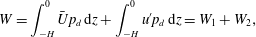
3 Energy conservation and energy flux
In the following we work in an accelerating reference frame moving with the far-field barotropic tidal current
 $\bar{U}_{b}(t)$
. In this reference frame the horizontal coordinate is
$\bar{U}_{b}(t)$
. In this reference frame the horizontal coordinate is
 $$\begin{eqnarray}\unicode[STIX]{x1D709}=x-\int _{0}^{t}\bar{U}_{b}(t^{\prime })\,\text{d}t^{\prime }=x-\frac{U_{0}}{\unicode[STIX]{x1D714}_{0}}\sin (\unicode[STIX]{x1D714}_{0}t)\end{eqnarray}$$
and the horizontal current is
 $$\begin{eqnarray}\tilde{u} (\unicode[STIX]{x1D709},z,t)=u(x(\unicode[STIX]{x1D709},t),z,t)-\bar{U}_{b}(t).\end{eqnarray}$$
We define a new pressure term via
 $$\begin{eqnarray}\tilde{p}=p(x(\unicode[STIX]{x1D709},t),z,t)+\frac{\text{d}\bar{U}_{b}}{\text{d}t}\unicode[STIX]{x1D709}.\end{eqnarray}$$
This removes the part of the horizontal pressure gradient which drives the barotropic tide in the far field. More generally, let tildes denote functions in the new reference frame, i.e.
 $\tilde{w}(\unicode[STIX]{x1D709},z,t)=w(x(\unicode[STIX]{x1D709},t),z,t)$
, etc. Under this change of variables the governing equations in the new reference frame are identical to (2.1a
)–(2.1d
) except for the addition of tildes to all dependent variables and with derivatives with respect to
$\tilde{w}(\unicode[STIX]{x1D709},z,t)=w(x(\unicode[STIX]{x1D709},t),z,t)$
, etc. Under this change of variables the governing equations in the new reference frame are identical to (2.1a
)–(2.1d
) except for the addition of tildes to all dependent variables and with derivatives with respect to
 $x$
replaced by derivatives with respect to
$x$
replaced by derivatives with respect to
 $\unicode[STIX]{x1D709}$
. The lower boundary is now moving and is at
$\unicode[STIX]{x1D709}$
. The lower boundary is now moving and is at
 $$\begin{eqnarray}z=-H+\tilde{h}(\unicode[STIX]{x1D709},t)=-H+h(x(\unicode[STIX]{x1D709},t))=-H+h\left(\unicode[STIX]{x1D709}+\int _{0}^{t}\bar{U}_{b}(t^{\prime })\,\text{d}t^{\prime }\right)\end{eqnarray}$$
and the bottom boundary condition is
 $$\begin{eqnarray}\tilde{\boldsymbol{u}}\boldsymbol{\cdot }\hat{n}=-(\bar{U}_{b}(t),0)\cdot \hat{n}\quad \text{at }z=-H+\tilde{h}(\unicode[STIX]{x1D709},t).\end{eqnarray}$$
Henceforth we will drop the tildes except for
 $\tilde{h}$
as both
$\tilde{h}$
as both
 $\tilde{h}(\unicode[STIX]{x1D709},t)$
and
$\tilde{h}(\unicode[STIX]{x1D709},t)$
and
 $h(x)$
will be used.
$h(x)$
will be used.
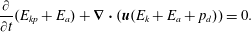
Neglecting viscous and diffusive effects the energy equation is
 $$\begin{eqnarray}\frac{\unicode[STIX]{x2202}}{\unicode[STIX]{x2202}t}(E_{k}+E_{a})+\unicode[STIX]{x1D735}\boldsymbol{\cdot }(\boldsymbol{u}(E_{k}+E_{a}+p_{d}))=0,\end{eqnarray}$$
where
 $p_{d}$
is the pressure perturbation (or disturbance) relative to the hydrostatic pressure of the undisturbed flow
$p_{d}$
is the pressure perturbation (or disturbance) relative to the hydrostatic pressure of the undisturbed flow
 $\bar{p}(z)$
,
$\bar{p}(z)$
,
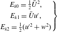
 $$\begin{eqnarray}E_{k}={\textstyle \frac{1}{2}}(u^{2}+w^{2})\end{eqnarray}$$
is the kinetic energy density (all energies are per unit mass) and
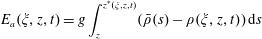 $$\begin{eqnarray}E_{a}(\unicode[STIX]{x1D709},z,t)=g\int _{z}^{z^{\ast }(\unicode[STIX]{x1D709},z,t)}(\bar{\unicode[STIX]{x1D70C}}(s)-\unicode[STIX]{x1D70C}(\unicode[STIX]{x1D709},z,t))\,\text{d}s\end{eqnarray}$$
is the available potential energy density (Holliday & McIntyre Reference Holliday and McIntyre1981; Shepherd Reference Shepherd1993). Here
 $\bar{\unicode[STIX]{x1D70C}}(z)$
is the reference density and
$\bar{\unicode[STIX]{x1D70C}}(z)$
is the reference density and
 $z^{\ast }(\unicode[STIX]{x1D709},z,t)$
is the height of the fluid particle at
$z^{\ast }(\unicode[STIX]{x1D709},z,t)$
is the height of the fluid particle at
 $(\unicode[STIX]{x1D709},z,t)$
in the reference stratification (Scotti, Beardsley & Butman Reference Scotti, Beardsley and Butman2006; Lamb Reference Lamb2007, Reference Lamb2008; Lamb & Nguyen Reference Lamb and Nguyen2009). We use the background stratification as the reference density which is appropriate for calculating the available potential energy in an infinitely long domain (Lamb Reference Lamb2008). It avoids sorting the density field which is computationally expensive. Since the background stratification is uniform, the available potential energy density has a simple analytic expression, namely
$(\unicode[STIX]{x1D709},z,t)$
in the reference stratification (Scotti, Beardsley & Butman Reference Scotti, Beardsley and Butman2006; Lamb Reference Lamb2007, Reference Lamb2008; Lamb & Nguyen Reference Lamb and Nguyen2009). We use the background stratification as the reference density which is appropriate for calculating the available potential energy in an infinitely long domain (Lamb Reference Lamb2008). It avoids sorting the density field which is computationally expensive. Since the background stratification is uniform, the available potential energy density has a simple analytic expression, namely
 $$\begin{eqnarray}E_{a}=\frac{1}{2}\frac{g^{2}\unicode[STIX]{x1D70C}^{\prime 2}}{N^{2}},\end{eqnarray}$$
where
 $\unicode[STIX]{x1D70C}^{\prime }$
is the density perturbation.
$\unicode[STIX]{x1D70C}^{\prime }$
is the density perturbation.
Let
 $$\begin{eqnarray}u=\bar{U}(z)+u^{\prime },\end{eqnarray}$$
where
 $u^{\prime }$
is the horizontal velocity perturbation. Far from the ridge
$u^{\prime }$
is the horizontal velocity perturbation. Far from the ridge
 $u^{\prime }$
is the wave-induced current; however, over the ridge it includes a barotropic contribution due to the constriction of the tidal flow over the ridge.
$u^{\prime }$
is the wave-induced current; however, over the ridge it includes a barotropic contribution due to the constriction of the tidal flow over the ridge.
We split the kinetic energy density into three terms
 $$\begin{eqnarray}E_{k}=E_{k0}+E_{k1}+E_{k2},\end{eqnarray}$$
where
 $$\begin{eqnarray}\displaystyle \left.\begin{array}{@{}c@{}}E_{k0}=\frac{1}{2}\bar{U}^{2},\\ E_{k1}=\bar{U}u^{\prime },\\ E_{k2}=\frac{1}{2}(u^{\prime 2}+w^{2})\end{array}\right\} & & \displaystyle\end{eqnarray}$$
are the contributions to the kinetic energy density which are of order zero, one and two in the perturbation velocities. We will refer to
 $$\begin{eqnarray}E_{kp}=E_{k1}+E_{k2},\end{eqnarray}$$
as the perturbation kinetic energy density. Since
 $\bar{U}$
is independent of time the energy equation can be written as
$\bar{U}$
is independent of time the energy equation can be written as
 $$\begin{eqnarray}\frac{\unicode[STIX]{x2202}}{\unicode[STIX]{x2202}t}(E_{kp}+E_{a})+\unicode[STIX]{x1D735}\boldsymbol{\cdot }(\boldsymbol{u}(E_{k}+E_{a}+p_{d}))=0.\end{eqnarray}$$
The perturbation kinetic energy can be negative if
 $E_{k1}$
dominates and is negative (Lamb Reference Lamb2010). We do not work with the positive definite wave energy
$E_{k1}$
dominates and is negative (Lamb Reference Lamb2010). We do not work with the positive definite wave energy
 $E_{k2}+E_{a}$
as this is not a conserved quantity. Use of wave energy, which is the energy associated with the wave in a reference frame moving with the background current, has proved to be a useful quantity in the context of wave packets propagating through a slowly varying background field. As a wave packet moves through a sheared background current wave energy is exchanged with the slowly varying background current and wave action is conserved (Broutman, Rottman & Eckermann Reference Broutman, Rottman and Eckermann2004). In our situation the majority of the energy is in low vertical modes which have wavelengths comparable to the water depth and the background sheared current does not vary slowly compared to this length scale.
$E_{k2}+E_{a}$
as this is not a conserved quantity. Use of wave energy, which is the energy associated with the wave in a reference frame moving with the background current, has proved to be a useful quantity in the context of wave packets propagating through a slowly varying background field. As a wave packet moves through a sheared background current wave energy is exchanged with the slowly varying background current and wave action is conserved (Broutman, Rottman & Eckermann Reference Broutman, Rottman and Eckermann2004). In our situation the majority of the energy is in low vertical modes which have wavelengths comparable to the water depth and the background sheared current does not vary slowly compared to this length scale.
In the following we use bars to indicate energy values integrated over a domain
 $$\begin{eqnarray}{\mathcal{D}}=[\unicode[STIX]{x1D709}_{l},\unicode[STIX]{x1D709}_{r}]\times [-H+\tilde{h}(\unicode[STIX]{x1D709},t),0],\end{eqnarray}$$
which is bounded by stationary lateral boundaries at
 $\unicode[STIX]{x1D709}=\unicode[STIX]{x1D709}_{l}$
and
$\unicode[STIX]{x1D709}=\unicode[STIX]{x1D709}_{l}$
and
 $\unicode[STIX]{x1D709}_{r}$
, by the moving bottom at
$\unicode[STIX]{x1D709}_{r}$
, by the moving bottom at
 $z_{b}=-H+\tilde{h}(\unicode[STIX]{x1D709},t)$
and the rigid lid at
$z_{b}=-H+\tilde{h}(\unicode[STIX]{x1D709},t)$
and the rigid lid at
 $z=0$
. We assume that the lateral boundaries are always far from the ridge where the water depth is
$z=0$
. We assume that the lateral boundaries are always far from the ridge where the water depth is
 $H$
. Let
$H$
. Let
 $$\begin{eqnarray}\bar{E}=\iint _{{\mathcal{D}}}E_{kp}+E_{a}\,\text{d}\unicode[STIX]{x1D709}\,\text{d}z\end{eqnarray}$$
be the total perturbation energy. Taking the time derivative and making use of (3.14) and the boundary conditions
 $\tilde{\boldsymbol{u}}\boldsymbol{\cdot }\hat{n}=0$
along the upper boundary and
$\tilde{\boldsymbol{u}}\boldsymbol{\cdot }\hat{n}=0$
along the upper boundary and
 $\boldsymbol{u}\boldsymbol{\cdot }\hat{n}\,\text{d}s=-\bar{U}_{b}h^{\prime }\,\text{d}x$
along the lower boundary, leads to
$\boldsymbol{u}\boldsymbol{\cdot }\hat{n}\,\text{d}s=-\bar{U}_{b}h^{\prime }\,\text{d}x$
along the lower boundary, leads to
 $$\begin{eqnarray}\left.\frac{\text{d}\bar{E}}{\text{d}t}=(KE_{f}+APE_{f}+W)\right|_{\unicode[STIX]{x1D709}_{r}}^{\unicode[STIX]{x1D709}_{\ell }}+\bar{U}_{b}(t)\int _{\unicode[STIX]{x1D709}_{l}}^{\unicode[STIX]{x1D709}_{r}}p_{b}h^{\prime }(x(\unicode[STIX]{x1D709},t))\,\text{d}\unicode[STIX]{x1D709},\end{eqnarray}$$
where
 $p_{b}(\unicode[STIX]{x1D709},t)=p_{d}(\unicode[STIX]{x1D709},-H+\tilde{h}(\unicode[STIX]{x1D709},t),t)$
is the pressure perturbation evaluated along the bottom. Here
$p_{b}(\unicode[STIX]{x1D709},t)=p_{d}(\unicode[STIX]{x1D709},-H+\tilde{h}(\unicode[STIX]{x1D709},t),t)$
is the pressure perturbation evaluated along the bottom. Here
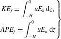 $$\begin{eqnarray}\left.\begin{array}{@{}c@{}}\displaystyle KE_{f}=\int _{-H}^{0}uE_{k}\,\text{d}z,\\ \displaystyle APE_{f}=\int _{-H}^{0}uE_{a}\,\text{d}z\end{array}\right\}\end{eqnarray}$$
are the vertically integrated kinetic and available potential energy flux densities, and
 $$\begin{eqnarray}W=\int _{-H}^{0}up_{d}\,\text{d}z\end{eqnarray}$$
is the rate work is done by the pressure perturbation. We will refer to this as the work term. The total energy flux through a horizontal location
 $x$
is
$x$
is
 $E_{f}=KE_{f}+APE_{f}+W$
. The last term on the right-hand side of (3.17) is the generation, or conversion, term
$E_{f}=KE_{f}+APE_{f}+W$
. The last term on the right-hand side of (3.17) is the generation, or conversion, term
 $G$
(Khatiwala Reference Khatiwala2003; Kelly, Nash & Kunze Reference Kelly, Nash and Kunze2010), which after integrating by parts (assuming
$G$
(Khatiwala Reference Khatiwala2003; Kelly, Nash & Kunze Reference Kelly, Nash and Kunze2010), which after integrating by parts (assuming
 $h(\unicode[STIX]{x1D709}_{l})=h(\unicode[STIX]{x1D709}_{r})=0$
) can be written as
$h(\unicode[STIX]{x1D709}_{l})=h(\unicode[STIX]{x1D709}_{r})=0$
) can be written as
 $$\begin{eqnarray}G=\bar{U}_{b}(t)\int _{\unicode[STIX]{x1D709}_{l}}^{\unicode[STIX]{x1D709}_{r}}p_{b}h^{\prime }(x(\unicode[STIX]{x1D709},t))\,\text{d}\unicode[STIX]{x1D709}=-\bar{U}_{b}(t)\left.\int _{\unicode[STIX]{x1D709}_{l}}^{\unicode[STIX]{x1D709}_{r}}(p_{\unicode[STIX]{x1D709}}+p_{z}h^{\prime })\right|_{z_{b}}h(x(\unicode[STIX]{x1D709},t))\,\text{d}\unicode[STIX]{x1D709}.\end{eqnarray}$$
The latter form is useful because the numerical model solves for the pressure gradients, not the pressure. Equation (3.17) states that the rate of change of energy in the domain
 ${\mathcal{D}}$
is balanced by the flux of energy through the lateral boundaries plus the rate energy is injected into the system through the generation term which in the moving reference frame is the work done moving the topography.
${\mathcal{D}}$
is balanced by the flux of energy through the lateral boundaries plus the rate energy is injected into the system through the generation term which in the moving reference frame is the work done moving the topography.
In linear theory in the absence of a background current (3.17) would simplify to
 $$\begin{eqnarray}\left.\frac{\text{d}\bar{E}}{\text{d}t}=W\right|_{\unicode[STIX]{x1D709}_{r}}^{\unicode[STIX]{x1D709}_{\ell }}+\bar{U}_{b}(t)\int _{\unicode[STIX]{x1D709}_{l}}^{\unicode[STIX]{x1D709}_{r}}p_{d}h^{\prime }(x(\unicode[STIX]{x1D709},t))\,\text{d}\unicode[STIX]{x1D709}\end{eqnarray}$$
because
 $E_{k}$
and
$E_{k}$
and
 $E_{a}$
are second-order, and
$E_{a}$
are second-order, and
 $p_{d}$
is first-order, in the perturbations. The energy fluxes
$p_{d}$
is first-order, in the perturbations. The energy fluxes
 $KE_{f}$
and
$KE_{f}$
and
 $APE_{f}$
, which would then be third-order in amplitude, do not appear in linear theory. This is not the case when there is a background current. As the only flux term that appears in (3.21) is
$APE_{f}$
, which would then be third-order in amplitude, do not appear in linear theory. This is not the case when there is a background current. As the only flux term that appears in (3.21) is
 $W$
, this term is often called the energy flux (Llewellyn Smith & Young Reference Llewellyn Smith and Young2002; Khatiwala Reference Khatiwala2003; Nash, Alford & Kunze Reference Nash, Alford and Kunze2005).
$W$
, this term is often called the energy flux (Llewellyn Smith & Young Reference Llewellyn Smith and Young2002; Khatiwala Reference Khatiwala2003; Nash, Alford & Kunze Reference Nash, Alford and Kunze2005).
Using
 $u=\bar{U}(z)+u^{\prime }$
we can split
$u=\bar{U}(z)+u^{\prime }$
we can split
 $KE_{f}$
into terms of order 0–3 in the perturbation velocity fields via
$KE_{f}$
into terms of order 0–3 in the perturbation velocity fields via
 $$\begin{eqnarray}\displaystyle KE_{f} & = & \displaystyle \frac{1}{2}\int _{-H}^{0}\bar{U}^{3}\,\text{d}z+\frac{3}{2}\int _{-H}^{0}\bar{U}^{2}u^{\prime }\,\text{d}z\nonumber\\ \displaystyle & & \displaystyle +\,\frac{1}{2}\int _{-H}^{0}\bar{U}(3u^{\prime 2}+w^{2})\,\text{d}z+\frac{1}{2}\int _{-H}^{0}u^{\prime }(u^{\prime 2}+w^{2})\,\text{d}z.\end{eqnarray}$$
The first term can be ignored as it is independent of
 $x$
and
$x$
and
 $t$
hence the values at
$t$
hence the values at
 $\unicode[STIX]{x1D709}_{l}$
and
$\unicode[STIX]{x1D709}_{l}$
and
 $\unicode[STIX]{x1D709}_{r}$
cancel. Henceforth
$\unicode[STIX]{x1D709}_{r}$
cancel. Henceforth
 $KE_{f}$
excludes this term. We split the remaining contributions into parts that are first-, second- and third-order in the perturbation velocities:
$KE_{f}$
excludes this term. We split the remaining contributions into parts that are first-, second- and third-order in the perturbation velocities:
 $$\begin{eqnarray}\left.\begin{array}{@{}c@{}}\displaystyle KE_{f1}=\frac{3}{2}\int _{-H}^{0}\bar{U}^{2}u^{\prime }\,\text{d}z,\\ \displaystyle KE_{f2}=\int _{-H}^{0}\bar{U}\left(\frac{3}{2}u^{\prime 2}+\frac{1}{2}w^{2}\right)\,\text{d}z,\\ \displaystyle KE_{f3}=\frac{1}{2}\int _{-H}^{0}u^{\prime }(u^{\prime 2}+w^{2})\,\text{d}z.\end{array}\right\}\end{eqnarray}$$
In our simulations the third-order term and the contribution from
 $w^{2}$
to the second-order term are negligible.
$w^{2}$
to the second-order term are negligible.
The work term
 $W$
can be split into two terms via
$W$
can be split into two terms via
 $$\begin{eqnarray}W=\int _{-H}^{0}\bar{U}p_{d}\,\text{d}z+\int _{-H}^{0}u^{\prime }p_{d}\,\text{d}z=W_{1}+W_{2},\end{eqnarray}$$
with
 $W_{1}$
and
$W_{1}$
and
 $W_{2}$
being of first and second order in the perturbation fields
$W_{2}$
being of first and second order in the perturbation fields
 $p_{d}$
and
$p_{d}$
and
 $u^{\prime }$
. Both make leading-order contributions to the tidally averaged work term because of the generation of second-order mean pressure fields.
$u^{\prime }$
. Both make leading-order contributions to the tidally averaged work term because of the generation of second-order mean pressure fields.
Linear hydrostatic theory for linear stratifications in the absence of a background current predicts that the energy fluxes scale with
 $$\begin{eqnarray}F_{0}={\textstyle \frac{1}{2}}NU_{0}^{2}h_{0}^{2},\end{eqnarray}$$
along with other factors depending on, for example, the ridge shape (Llewellyn Smith & Young Reference Llewellyn Smith and Young2002; Garrett & Kunze Reference Garrett and Kunze2007), hence we will non-dimensionalize our energy fluxes by scaling them by
 $F_{0}$
.
$F_{0}$
.
4 Linear theory
In this section we develop a linear theory to predict the waves that are generated by periodic tidal flow over an isolated bathymetric feature in the presence of a steady surface trapped background current restricted to lie above the bathymetry so that waves are generated solely by tide–topography interactions. As mentioned above rotational effects are not included. The stratification and current are assumed to be stable (Richardson number greater than
 $1/4$
) but are otherwise arbitrary. We follow the procedure used by Khatiwala (Reference Khatiwala2003) and assume that the tidal flow consists of a single tidal constituent and seek periodic solutions. Multiple constituents can be considered via linear superposition. One difference between the fully nonlinear numerical simulations and the linear theory is that the former is an initial value problem while the latter is a periodic solution which can be viewed as the wave field in the limit
$1/4$
) but are otherwise arbitrary. We follow the procedure used by Khatiwala (Reference Khatiwala2003) and assume that the tidal flow consists of a single tidal constituent and seek periodic solutions. Multiple constituents can be considered via linear superposition. One difference between the fully nonlinear numerical simulations and the linear theory is that the former is an initial value problem while the latter is a periodic solution which can be viewed as the wave field in the limit
 $t\rightarrow \infty$
.
$t\rightarrow \infty$
.
As in the previous section we use a reference frame moving with the far field tidal current
 $\bar{U}_{b}(t)$
. We assume small amplitude topography and waves and linearize about a steady background horizontal current
$\bar{U}_{b}(t)$
. We assume small amplitude topography and waves and linearize about a steady background horizontal current
 $\bar{U}(z)$
. This leads to the well-known equation for the vertical velocity
$\bar{U}(z)$
. This leads to the well-known equation for the vertical velocity
 $$\begin{eqnarray}\left(\frac{\unicode[STIX]{x2202}}{\unicode[STIX]{x2202}t}+\bar{U}\frac{\unicode[STIX]{x2202}}{\unicode[STIX]{x2202}\unicode[STIX]{x1D709}}\right)^{2}\unicode[STIX]{x1D6FB}^{2}w-\frac{\text{d}^{2}\bar{U}}{\text{d}z^{2}}\left(\frac{\unicode[STIX]{x2202}}{\unicode[STIX]{x2202}t}+\bar{U}\frac{\unicode[STIX]{x2202}}{\unicode[STIX]{x2202}\unicode[STIX]{x1D709}}\right)w_{\unicode[STIX]{x1D709}}+N^{2}(z)w_{\unicode[STIX]{x1D709}\unicode[STIX]{x1D709}}=0,\end{eqnarray}$$
where the buoyancy frequency
 $N$
is given by
$N$
is given by
 $$\begin{eqnarray}N^{2}(z)=-g\frac{\text{d}\bar{\unicode[STIX]{x1D70C}}}{\text{d}z},\end{eqnarray}$$
which for the theory is an arbitrary non-negative function of
 $z$
. The linearized bottom boundary condition is
$z$
. The linearized bottom boundary condition is
 $$\begin{eqnarray}w=\bar{U}_{b}(t)\tilde{h}_{\unicode[STIX]{x1D709}}=\bar{U}_{b}(t)h^{\prime }(x(\unicode[STIX]{x1D709},t))\quad \text{at }z=-H.\end{eqnarray}$$
Searching for solutions of the form
 $$\begin{eqnarray}w=\text{e}^{\text{i}(k\unicode[STIX]{x1D709}-\unicode[STIX]{x1D714}t)}\unicode[STIX]{x1D719}(z)\end{eqnarray}$$
we obtain the Taylor–Goldstein equation for the vertical structure
 $\unicode[STIX]{x1D719}(z)$
,
$\unicode[STIX]{x1D719}(z)$
,
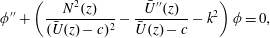 $$\begin{eqnarray}\unicode[STIX]{x1D719}^{\prime \prime }+\left(\frac{N^{2}(z)}{(\bar{U}(z)-c)^{2}}-\frac{\bar{U}^{\prime \prime }(z)}{\bar{U}(z)-c}-k^{2}\right)\unicode[STIX]{x1D719}=0,\end{eqnarray}$$
where
 $c=\unicode[STIX]{x1D714}/k$
and primes denote differentiation with respect to
$c=\unicode[STIX]{x1D714}/k$
and primes denote differentiation with respect to
 $z$
. Solutions satisfying the homogeneous boundary conditions
$z$
. Solutions satisfying the homogeneous boundary conditions
 $\unicode[STIX]{x1D719}(-H)=\unicode[STIX]{x1D719}(0)=0$
consist of two types: the discrete spectrum, or eigenmodes,
$\unicode[STIX]{x1D719}(-H)=\unicode[STIX]{x1D719}(0)=0$
consist of two types: the discrete spectrum, or eigenmodes,
 $\{\unicode[STIX]{x1D719}_{n}^{\pm },c_{n}^{\pm }\}$
with phase speeds
$\{\unicode[STIX]{x1D719}_{n}^{\pm },c_{n}^{\pm }\}$
with phase speeds
 $c_{n}^{+}>\max \{\bar{U}\}$
or
$c_{n}^{+}>\max \{\bar{U}\}$
or
 $c_{n}^{-}<\min \{\bar{U}\}$
; and the continuous spectrum with
$c_{n}^{-}<\min \{\bar{U}\}$
; and the continuous spectrum with
 $c\in [\min \{\bar{U}\},\max \{\bar{U}\}]$
. Figure 4 is a schematic showing the discrete and continuous spectrums when
$c\in [\min \{\bar{U}\},\max \{\bar{U}\}]$
. Figure 4 is a schematic showing the discrete and continuous spectrums when
 $U_{min}<0<U_{max}$
.
$U_{min}<0<U_{max}$
.

Figure 4. Spectrum of the Taylor–Goldstein equation for frequency
 $\unicode[STIX]{x1D714}>0$
. Shown are the first four positive and negative eigenvalues
$\unicode[STIX]{x1D714}>0$
. Shown are the first four positive and negative eigenvalues
 $k_{n}^{+}$
and
$k_{n}^{+}$
and
 $k_{n}^{-}$
(the discrete spectrum) with limit points at
$k_{n}^{-}$
(the discrete spectrum) with limit points at
 $\unicode[STIX]{x1D714}/U_{max}$
and
$\unicode[STIX]{x1D714}/U_{max}$
and
 $\unicode[STIX]{x1D714}/U_{min}$
respectively. Also shown is point in the continuous spectrum
$\unicode[STIX]{x1D714}/U_{min}$
respectively. Also shown is point in the continuous spectrum
 $k_{c}=\unicode[STIX]{x1D714}/U(z)$
for a value of
$k_{c}=\unicode[STIX]{x1D714}/U(z)$
for a value of
 $z$
for which
$z$
for which
 $0<U(z)<U_{max}$
. The grey bars indicate regions where the continuous spectrum lies: as
$0<U(z)<U_{max}$
. The grey bars indicate regions where the continuous spectrum lies: as
 $z$
varies across the water depth
$z$
varies across the water depth
 $k_{c}$
sweeps out the grey regions
$k_{c}$
sweeps out the grey regions
 $k<\unicode[STIX]{x1D714}/U_{min}$
and
$k<\unicode[STIX]{x1D714}/U_{min}$
and
 $k>\unicode[STIX]{x1D714}/U_{max}$
. As
$k>\unicode[STIX]{x1D714}/U_{max}$
. As
 $U_{min}\rightarrow 0$
the limit point at
$U_{min}\rightarrow 0$
the limit point at
 $\unicode[STIX]{x1D714}/U_{min}\rightarrow -\infty$
.
$\unicode[STIX]{x1D714}/U_{min}\rightarrow -\infty$
.
We use the Fourier transform defined as
 $$\begin{eqnarray}\hat{f}(k)=\int _{-\infty }^{\infty }f(\unicode[STIX]{x1D709})\text{e}^{-\text{i}k\unicode[STIX]{x1D709}}\,\text{d}\unicode[STIX]{x1D709}\end{eqnarray}$$
to transform the bottom boundary condition (4.3), yielding (Bell Reference Bell1975a ; Khatiwala Reference Khatiwala2003)
 $$\begin{eqnarray}{\hat{w}}(k,-H,t)=-{\hat{h}}(k)\mathop{\sum }_{n=-\infty }^{\infty }\text{i}n\unicode[STIX]{x1D714}_{0}\text{J}_{n}\left(\frac{-kU_{0}}{\unicode[STIX]{x1D714}_{0}}\right)\text{e}^{-\text{i}n\unicode[STIX]{x1D714}_{0}t},\end{eqnarray}$$
where the tidal current is
 $$\begin{eqnarray}\bar{U}_{b}(t)=U_{0}\text{e}^{\text{i}\unicode[STIX]{x1D714}_{0}t}\end{eqnarray}$$
and
 $\text{J}_{n}$
is the Bessel function of the first kind of order
$\text{J}_{n}$
is the Bessel function of the first kind of order
 $n$
. Based on this we look for a series solution for
$n$
. Based on this we look for a series solution for
 ${\hat{w}}(k,z,t)$
of the form
${\hat{w}}(k,z,t)$
of the form
 $$\begin{eqnarray}{\hat{w}}(k,z,t)=-\mathop{\sum }_{n=-\infty }^{\infty }\text{i}n\unicode[STIX]{x1D714}_{0}{\hat{h}}(k)\text{J}_{n}\left(\frac{-kU_{0}}{\unicode[STIX]{x1D714}_{0}}\right)W_{n}(k,z)\text{e}^{-\text{i}n\unicode[STIX]{x1D714}_{0}t},\end{eqnarray}$$
where the functions
 $W_{n}(k,z)$
are solutions of the Taylor–Goldstein equation for waves of frequency
$W_{n}(k,z)$
are solutions of the Taylor–Goldstein equation for waves of frequency
 $n\unicode[STIX]{x1D714}_{0}$
,
$n\unicode[STIX]{x1D714}_{0}$
,
 $$\begin{eqnarray}{\mathcal{L}}_{n}[W_{n}]\equiv W_{n}^{\prime \prime }+\left(\frac{k^{2}N^{2}(z)}{(n\unicode[STIX]{x1D714}_{0}-k\bar{U}(z))^{2}}+k\frac{\bar{U}^{\prime \prime }(z)}{(n\unicode[STIX]{x1D714}_{0}-k\bar{U}(z))}-k^{2}\right)W_{n}=0,\end{eqnarray}$$
satisfying the boundary conditions
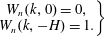 $$\begin{eqnarray}\left.\begin{array}{@{}c@{}}W_{n}(k,0)=0,\\ W_{n}(k,-H)=1.\end{array}\right\}\end{eqnarray}$$
So far the derivation has followed Khatiwala (Reference Khatiwala2003) who considered constant
 $N$
and did not include background currents. Under these conditions the Taylor–Goldstein equation can be solved analytically. With a sheared background current or non-constant
$N$
and did not include background currents. Under these conditions the Taylor–Goldstein equation can be solved analytically. With a sheared background current or non-constant
 $N(z)$
equations (4.10)–(4.11) must be solved numerically. To do so we numerically solve the initial value problem
$N(z)$
equations (4.10)–(4.11) must be solved numerically. To do so we numerically solve the initial value problem
 $$\begin{eqnarray}\left.\begin{array}{@{}c@{}}{\mathcal{L}}_{n}[\unicode[STIX]{x1D719}_{n}]=0,\\ \unicode[STIX]{x1D719}_{n}(k,0)=0,\\ \unicode[STIX]{x1D719}_{n}^{\prime }(k,0)=1\end{array}\right\}\end{eqnarray}$$
to get
 $\unicode[STIX]{x1D719}_{n}(k,z)$
on
$\unicode[STIX]{x1D719}_{n}(k,z)$
on
 $z\in [-H,0]$
and then let
$z\in [-H,0]$
and then let
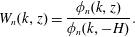 $$\begin{eqnarray}W_{n}(k,z)=\frac{\unicode[STIX]{x1D719}_{n}(k,z)}{\unicode[STIX]{x1D719}_{n}(k,-H)}.\end{eqnarray}$$
Here
 $k$
varies continuously over the real line. The values of
$k$
varies continuously over the real line. The values of
 $k$
for which
$k$
for which
 $\unicode[STIX]{x1D719}_{n}(k,-H)=0$
give the eigenmodes, for which
$\unicode[STIX]{x1D719}_{n}(k,-H)=0$
give the eigenmodes, for which
 $W_{n}$
is singular.
$W_{n}$
is singular.
Taking the inverse Fourier transform of (4.9) we obtain
 $$\begin{eqnarray}w(\unicode[STIX]{x1D709},z,t)=\mathop{\sum }_{\stackrel{-\infty }{n\neq 0}}^{\infty }\frac{-\text{i}n\unicode[STIX]{x1D714}_{0}}{2\unicode[STIX]{x03C0}}\text{e}^{-\text{i}n\unicode[STIX]{x1D714}_{0}t}\int _{-\infty }^{\infty }{\hat{h}}(k)\text{J}_{n}\left(\frac{-kU_{0}}{\unicode[STIX]{x1D714}_{0}}\right)\frac{\unicode[STIX]{x1D719}_{n}(k,z)}{\unicode[STIX]{x1D719}_{n}(k,-H)}\text{e}^{\text{i}k\unicode[STIX]{x1D709}}\,\text{d}k.\end{eqnarray}$$
The contributions to the integral are of two types: (i) contributions from the poles where
 $\unicode[STIX]{x1D719}_{n}(k,-H)=0$
and (ii) possibly from the continuous spectrum. Without loss of generality we will assume that
$\unicode[STIX]{x1D719}_{n}(k,-H)=0$
and (ii) possibly from the continuous spectrum. Without loss of generality we will assume that
 $U_{min}=\min \{\bar{U}\}\leqslant 0$
and
$U_{min}=\min \{\bar{U}\}\leqslant 0$
and
 $U_{max}=\max \{\bar{U}\}>0$
. In this paper we do not consider the continuous spectrum as the wave field appears to be well predicted by the discrete spectrum alone.
$U_{max}=\max \{\bar{U}\}>0$
. In this paper we do not consider the continuous spectrum as the wave field appears to be well predicted by the discrete spectrum alone.
4.1 Contribution from the discrete spectrum
For
 $n\unicode[STIX]{x1D714}_{0}/U_{min}<k<n\unicode[STIX]{x1D714}_{0}/U_{max}$
, or, if
$n\unicode[STIX]{x1D714}_{0}/U_{min}<k<n\unicode[STIX]{x1D714}_{0}/U_{max}$
, or, if
 $U_{min}=0$
as is the case in our numerical simulations, for
$U_{min}=0$
as is the case in our numerical simulations, for
 $-\infty <k<n\unicode[STIX]{x1D714}_{0}/U_{max}$
, the contributions to the integral from the discrete spectrum come from the poles of the integrand, i.e. the values of
$-\infty <k<n\unicode[STIX]{x1D714}_{0}/U_{max}$
, the contributions to the integral from the discrete spectrum come from the poles of the integrand, i.e. the values of
 $k$
for which
$k$
for which
 $\unicode[STIX]{x1D719}_{n}(k,-H)=0$
. The corresponding
$\unicode[STIX]{x1D719}_{n}(k,-H)=0$
. The corresponding
 $\unicode[STIX]{x1D719}_{n}$
are the eigenmodes. Let
$\unicode[STIX]{x1D719}_{n}$
are the eigenmodes. Let
 $k_{nm}^{+}$
,
$k_{nm}^{+}$
,
 $m=1,2,\ldots \,$
be the positive zeros of
$m=1,2,\ldots \,$
be the positive zeros of
 $\unicode[STIX]{x1D719}_{n}(k,-H)$
and let
$\unicode[STIX]{x1D719}_{n}(k,-H)$
and let
 $k_{nm}^{-}$
,
$k_{nm}^{-}$
,
 $m=1,2,\ldots \,$
be the negative zeros. Ordering them in decreasing phase speed magnitude we have
$m=1,2,\ldots \,$
be the negative zeros. Ordering them in decreasing phase speed magnitude we have
 $$\begin{eqnarray}k_{n1}^{+}<k_{n2}^{+}<k_{n3}^{+}<\cdots \quad \text{with }k_{nm}^{+}\rightarrow \frac{n\unicode[STIX]{x1D714}_{0}}{U_{max}}\text{ as }m\rightarrow \infty\end{eqnarray}$$
and
 $$\begin{eqnarray}-k_{n1}^{-}<-k_{n2}^{-}<-k_{n3}^{-}<\cdots \quad \text{with }-k_{nm}^{-}\rightarrow -\frac{n\unicode[STIX]{x1D714}_{0}}{U_{min}}\text{ as }m\rightarrow \infty .\end{eqnarray}$$
In our examples with
 $U_{min}=0$
we have
$U_{min}=0$
we have
 $k_{nm}^{-}\rightarrow -\infty$
as
$k_{nm}^{-}\rightarrow -\infty$
as
 $m\rightarrow \infty$
. In the above
$m\rightarrow \infty$
. In the above
 $n$
refers to the wave harmonic, i.e. waves of frequency
$n$
refers to the wave harmonic, i.e. waves of frequency
 $n\unicode[STIX]{x1D714}_{0}$
, while
$n\unicode[STIX]{x1D714}_{0}$
, while
 $m$
is the eigenmode index. For positive/negative
$m$
is the eigenmode index. For positive/negative
 $n$
, the wavenumbers
$n$
, the wavenumbers
 $k_{nm}^{+}$
correspond to rightward/leftward propagating waves. This is reversed for wavenumbers
$k_{nm}^{+}$
correspond to rightward/leftward propagating waves. This is reversed for wavenumbers
 $k_{nm}^{-}$
.
$k_{nm}^{-}$
.
If
 $\{\unicode[STIX]{x1D719}_{n}(k,z),k\}$
is the solution of the Taylor–Goldstein equation subject to boundary conditions (4.12) for
$\{\unicode[STIX]{x1D719}_{n}(k,z),k\}$
is the solution of the Taylor–Goldstein equation subject to boundary conditions (4.12) for
 $\unicode[STIX]{x1D714}=n\unicode[STIX]{x1D714}_{0}$
then
$\unicode[STIX]{x1D714}=n\unicode[STIX]{x1D714}_{0}$
then
 $\{\unicode[STIX]{x1D719}_{n}(k,z),-k\}$
is a solution for
$\{\unicode[STIX]{x1D719}_{n}(k,z),-k\}$
is a solution for
 $\unicode[STIX]{x1D714}=-n\unicode[STIX]{x1D714}_{0}$
since the problem for
$\unicode[STIX]{x1D714}=-n\unicode[STIX]{x1D714}_{0}$
since the problem for
 $\unicode[STIX]{x1D719}$
is invariant under concurrent changes of the signs of
$\unicode[STIX]{x1D719}$
is invariant under concurrent changes of the signs of
 $\unicode[STIX]{x1D714}$
and
$\unicode[STIX]{x1D714}$
and
 $k$
. Thus
$k$
. Thus
 $$\begin{eqnarray}k_{nm}^{+}=-k_{-nm}^{-}\end{eqnarray}$$
and
 $$\begin{eqnarray}\unicode[STIX]{x1D719}_{n}(k,z)=\unicode[STIX]{x1D719}_{-n}(-k,z).\end{eqnarray}$$
Differentiating the latter gives
 $$\begin{eqnarray}\frac{\unicode[STIX]{x2202}\unicode[STIX]{x1D719}_{n}}{\unicode[STIX]{x2202}k}(k,z)=-\frac{\unicode[STIX]{x2202}\unicode[STIX]{x1D719}_{-n}}{\unicode[STIX]{x2202}k}(-k,z).\end{eqnarray}$$
Rightward propagating waves. Contributions to rightward propagating waves come from the positive eigenvalues for frequencies
 $n\unicode[STIX]{x1D714}_{0}>0$
and from the negative eigenvalues for frequencies
$n\unicode[STIX]{x1D714}_{0}>0$
and from the negative eigenvalues for frequencies
 $-n\unicode[STIX]{x1D714}_{0}<0$
(Khatiwala Reference Khatiwala2003). Use of the residue theorem and the symmetries given above leads to the following contributions to
$-n\unicode[STIX]{x1D714}_{0}<0$
(Khatiwala Reference Khatiwala2003). Use of the residue theorem and the symmetries given above leads to the following contributions to
 $u$
and
$u$
and
 $w$
from the discrete spectrum:
$w$
from the discrete spectrum:
 $$\begin{eqnarray}\displaystyle & \displaystyle w_{ds}(\unicode[STIX]{x1D709},z,t)=2\mathop{\sum }_{n=1}^{n_{0}}\mathop{\sum }_{m=1}^{\infty }\left\{n\unicode[STIX]{x1D714}_{0}\text{J}_{n}\left(\frac{-k_{nm}^{+}U_{0}}{\unicode[STIX]{x1D714}_{0}}\right)\frac{\unicode[STIX]{x1D719}_{n}(k_{nm}^{+},z)}{\displaystyle \frac{\unicode[STIX]{x2202}\unicode[STIX]{x1D719}_{n}}{\unicode[STIX]{x2202}k}(k_{nm}^{+},-H)}\text{Re}\{{\hat{h}}(k_{nm}^{+})\text{e}^{\text{i}(k_{nm}^{+}\unicode[STIX]{x1D709}-n\unicode[STIX]{x1D714}_{0}t)}\}\right\}, & \displaystyle \nonumber\\ \displaystyle & & \displaystyle\end{eqnarray}$$
 $$\begin{eqnarray}\displaystyle & \displaystyle u_{ds}(\unicode[STIX]{x1D709},z,t)=2\mathop{\sum }_{n=1}^{n_{0}}\mathop{\sum }_{m=1}^{\infty }\left\{n\unicode[STIX]{x1D714}_{0}\text{J}_{n}\left(\frac{-k_{nm}^{+}U_{0}}{\unicode[STIX]{x1D714}_{0}}\right)\frac{\unicode[STIX]{x1D719}_{n}^{\prime }(k_{nm}^{+},z)}{\displaystyle \frac{\unicode[STIX]{x2202}\unicode[STIX]{x1D719}_{n}}{\unicode[STIX]{x2202}k}(k_{nm}^{+},-H)}\text{Re}\left\{\text{i}\frac{{\hat{h}}(k_{nm}^{+})}{k_{nm}^{+}}\text{e}^{\text{i}(k_{nm}^{+}\unicode[STIX]{x1D709}-n\unicode[STIX]{x1D714}_{0}t)}\right\}\right\} & \displaystyle \nonumber\\ \displaystyle & & \displaystyle\end{eqnarray}$$
for
 $\unicode[STIX]{x1D709}>0$
. Here
$\unicode[STIX]{x1D709}>0$
. Here
 $\unicode[STIX]{x1D719}_{n}^{\prime }$
denotes differentiation with respect to
$\unicode[STIX]{x1D719}_{n}^{\prime }$
denotes differentiation with respect to
 $z$
.
$z$
.
Leftward propagating waves. For the leftward propagating waves we have
 $$\begin{eqnarray}\displaystyle & \displaystyle w_{ds}(\unicode[STIX]{x1D709},z,t)=-2\mathop{\sum }_{n=1}^{n_{0}}\mathop{\sum }_{m=1}^{\infty }\left\{n\unicode[STIX]{x1D714}_{0}\text{J}_{n}\left(\frac{-k_{nm}^{-}U_{0}}{\unicode[STIX]{x1D714}_{0}}\right)\frac{\unicode[STIX]{x1D719}_{n}(k_{nm}^{-},z)}{\displaystyle \frac{\unicode[STIX]{x2202}\unicode[STIX]{x1D719}_{n}}{\unicode[STIX]{x2202}k}(k_{nm}^{-},-H)}\text{Re}\{{\hat{h}}(k_{nm}^{-})\text{e}^{\text{i}(k_{nm}^{-}\unicode[STIX]{x1D709}-n\unicode[STIX]{x1D714}_{0}t)}\}\right\}, & \displaystyle \nonumber\\ \displaystyle & & \displaystyle\end{eqnarray}$$
 $$\begin{eqnarray}\displaystyle & \displaystyle u_{ds}(\unicode[STIX]{x1D709},z,t)=-2\mathop{\sum }_{n=1}^{n_{0}}\mathop{\sum }_{m=1}^{\infty }\left\{n\unicode[STIX]{x1D714}_{0}\text{J}_{n}\left(\frac{-k_{nm}^{-}U_{0}}{\unicode[STIX]{x1D714}_{0}}\right)\frac{\unicode[STIX]{x1D719}_{n}^{\prime }(k_{nm}^{-},z)}{\displaystyle \frac{\unicode[STIX]{x2202}\unicode[STIX]{x1D719}_{n}}{\unicode[STIX]{x2202}k}(k_{nm}^{-},-H)}\text{Re}\left\{\text{i}\frac{{\hat{h}}(k_{nm}^{-})}{k_{nm}^{-}}\text{e}^{\text{i}(k_{nm}^{-}\unicode[STIX]{x1D709}-n\unicode[STIX]{x1D714}_{0}t)}\right\}\right\} & \displaystyle \nonumber\\ \displaystyle & & \displaystyle\end{eqnarray}$$
for
 $\unicode[STIX]{x1D709}<0$
.
$\unicode[STIX]{x1D709}<0$
.
The sum over
 $n$
has an upper limit because eigenmodes only exist for a finite number of frequencies (e.g.
$n$
has an upper limit because eigenmodes only exist for a finite number of frequencies (e.g.
 $n\unicode[STIX]{x1D714}_{0}<N$
for
$n\unicode[STIX]{x1D714}_{0}<N$
for
 $N$
constant and
$N$
constant and
 $\bar{U}(z)=0$
).
$\bar{U}(z)=0$
).
To cast the results into non-dimensional terms, because the eigenmodes are scaled so that
 $\unicode[STIX]{x1D719}_{n}^{\prime }(k,0)=1$
, we take
$\unicode[STIX]{x1D719}_{n}^{\prime }(k,0)=1$
, we take
 $\unicode[STIX]{x1D719}_{n}^{\prime }$
to be dimensionless. Denoting dimensionless variables with a tilde we have
$\unicode[STIX]{x1D719}_{n}^{\prime }$
to be dimensionless. Denoting dimensionless variables with a tilde we have
 $$\begin{eqnarray}(\unicode[STIX]{x1D719}_{n},{\hat{h}},k,\unicode[STIX]{x1D714}_{0},U_{0})=\left(H\tilde{\unicode[STIX]{x1D719}}_{n},H^{2}\hat{\tilde{h}},\frac{\tilde{k}}{H},N\tilde{\unicode[STIX]{x1D714}_{0}},NH\tilde{U} _{0}\right).\end{eqnarray}$$
Figure 5 compares phase speeds for the first 20 modes for three different background currents (the maximum difference between the phase speeds and corresponding group velocities is less than 2 %). For the rightward propagating waves the phase speeds increase as current strength
 $U_{s}$
or depth
$U_{s}$
or depth
 $-z_{s}$
is increased, decreasing monotonically to
$-z_{s}$
is increased, decreasing monotonically to
 $U_{s}$
as the mode number
$U_{s}$
as the mode number
 $m\rightarrow \infty$
. The phase speeds of the upstream propagating waves decrease as the current is strengthened. They are much less sensitive to the strength or depth of the current. The phase speeds are not sensitive to the shear layer thickness
$m\rightarrow \infty$
. The phase speeds of the upstream propagating waves decrease as the current is strengthened. They are much less sensitive to the strength or depth of the current. The phase speeds are not sensitive to the shear layer thickness
 $d_{s}$
. Sample eigenmodes are shown in figure 6. For the leftward propagating modes
$d_{s}$
. Sample eigenmodes are shown in figure 6. For the leftward propagating modes
 $k<0$
and
$k<0$
and
 $\unicode[STIX]{x1D714}_{0}-\bar{U}k$
is larger in the current than beneath it, hence the higher modes oscillate more rapidly beneath the current. For the rightward propagating modes
$\unicode[STIX]{x1D714}_{0}-\bar{U}k$
is larger in the current than beneath it, hence the higher modes oscillate more rapidly beneath the current. For the rightward propagating modes
 $k>0$
and
$k>0$
and
 $\unicode[STIX]{x1D714}_{0}-\bar{U}k$
is smaller in the current. The higher modes now oscillate more rapidly in the current.
$\unicode[STIX]{x1D714}_{0}-\bar{U}k$
is smaller in the current. The higher modes now oscillate more rapidly in the current.

Figure 5. Wave phase speeds for waves of tidal frequency for various background currents. Horizontal lines indicate limiting values of
 $0.1$
and
$0.1$
and
 $0.16$
. Solid curves are phase speeds of rightward propagating waves. Dashed are phase speeds (absolute value) of leftward propagating waves.
$0.16$
. Solid curves are phase speeds of rightward propagating waves. Dashed are phase speeds (absolute value) of leftward propagating waves.
Figure 6. Eigenmodes (a,c) 1, 2, 4 and 8 and their derivatives (b,d) for waves of tidal frequency for background current used in sets 1–3 for which
 $(U_{s}/(NH),z_{s}/H,d_{s}/H)=(0.1,-0.3,-0.06)$
. (a,b) Leftward propagating waves. (c,d) Rightward propagating waves.
$(U_{s}/(NH),z_{s}/H,d_{s}/H)=(0.1,-0.3,-0.06)$
. (a,b) Leftward propagating waves. (c,d) Rightward propagating waves.
The presence of the current has a significant impact on the modal wavenumbers which in turn affects the relative contributions of the different modes. Contributions to
 $w_{ds}$
come from
$w_{ds}$
come from
 ${\hat{h}}(k)$
which depends only on the properties of the bathymetry,
${\hat{h}}(k)$
which depends only on the properties of the bathymetry,
 $\text{J}_{n}(-kU_{0}/\unicode[STIX]{x1D714}_{0})$
which depends on the tidal current amplitude
$\text{J}_{n}(-kU_{0}/\unicode[STIX]{x1D714}_{0})$
which depends on the tidal current amplitude
 $U_{0}$
and frequency
$U_{0}$
and frequency
 $\unicode[STIX]{x1D714}_{0}$
, and on the eigenmodes which are determined by the stratification and background currents. We now briefly consider the contributions from some of the factors in expressions (4.20)–(4.23).
$\unicode[STIX]{x1D714}_{0}$
, and on the eigenmodes which are determined by the stratification and background currents. We now briefly consider the contributions from some of the factors in expressions (4.20)–(4.23).
The Gaussian ridge (2.2) has Fourier transform
 $$\begin{eqnarray}{\hat{h}}(k)=\sqrt{\unicode[STIX]{x03C0}}ah_{0}\text{e}^{-((a^{2}k^{2})/4)}.\end{eqnarray}$$
Figure 7(a) shows
 $f_{1}={\hat{h}}(k)/{\hat{h}}(0)$
for
$f_{1}={\hat{h}}(k)/{\hat{h}}(0)$
for
 $a/H=1.2$
,
$a/H=1.2$
,
 $1.8$
,
$1.8$
,
 $2.4$
,
$2.4$
,
 $3.0$
and
$3.0$
and
 $3.6$
. As
$3.6$
. As
 $a/H$
increases the spectrum gets narrower. The values for the discrete spectrum for waves of tidal frequency from set 4 (see table 1) are indicated with red stars. Rightward propagating waves (
$a/H$
increases the spectrum gets narrower. The values for the discrete spectrum for waves of tidal frequency from set 4 (see table 1) are indicated with red stars. Rightward propagating waves (
 $k>0$
) have limiting wavenumber
$k>0$
) have limiting wavenumber
 $k_{lim}H=(\unicode[STIX]{x1D714}_{0}/U_{max})H\approx 1.4$
. For
$k_{lim}H=(\unicode[STIX]{x1D714}_{0}/U_{max})H\approx 1.4$
. For
 $a/H=1.2$
and
$a/H=1.2$
and
 $1.8$
all eigenmodes make a significant contribution. For the widest topography only the first 3 eigenmodes do. For the leftward propagating waves
$1.8$
all eigenmodes make a significant contribution. For the widest topography only the first 3 eigenmodes do. For the leftward propagating waves
 $k_{1m}^{-}\rightarrow -\infty$
as
$k_{1m}^{-}\rightarrow -\infty$
as
 $m\rightarrow \infty$
and fewer eigenmodes make a significant contribution.
$m\rightarrow \infty$
and fewer eigenmodes make a significant contribution.
These values are multiplied by
 $\text{J}_{1}(-(kU_{0}/\unicode[STIX]{x1D714}_{0}))$
. In our case
$\text{J}_{1}(-(kU_{0}/\unicode[STIX]{x1D714}_{0}))$
. In our case
 $U_{0}=U_{s}/10$
so this factor is equal to
$U_{0}=U_{s}/10$
so this factor is equal to
 $\text{J}_{1}(-(k/10k_{lim}))\approx k/20k_{lim}$
. Figure 7(b) shows
$\text{J}_{1}(-(k/10k_{lim}))\approx k/20k_{lim}$
. Figure 7(b) shows
 $f_{2}={\hat{h}}(k)\text{J}_{1}(-(kU_{0}/\unicode[STIX]{x1D714}_{0}))/{\hat{h}}(0)$
. The Bessel function makes contributions from higher harmonics negligible.
$f_{2}={\hat{h}}(k)\text{J}_{1}(-(kU_{0}/\unicode[STIX]{x1D714}_{0}))/{\hat{h}}(0)$
. The Bessel function makes contributions from higher harmonics negligible.
Including the contribution to the vertical velocity from
 $\unicode[STIX]{x2202}\unicode[STIX]{x1D719}_{n}/\unicode[STIX]{x2202}k$
(figure 7
c) we see that for narrow ridges several modes make higher contributions than mode-one does. The highest contributions to the horizontal velocity, which has an extra division by
$\unicode[STIX]{x2202}\unicode[STIX]{x1D719}_{n}/\unicode[STIX]{x2202}k$
(figure 7
c) we see that for narrow ridges several modes make higher contributions than mode-one does. The highest contributions to the horizontal velocity, which has an extra division by
 $k$
, are more skewed to the low modes. For
$k$
, are more skewed to the low modes. For
 $a/H=1.2$
and
$a/H=1.2$
and
 $1.8$
the largest contributions for the rightward propagating waves are from modes 2, 3 and 1 (figure 7
d). For wider ridges mode-one dominates. Trends are similar for the leftward propagating waves. The signs of the
$1.8$
the largest contributions for the rightward propagating waves are from modes 2, 3 and 1 (figure 7
d). For wider ridges mode-one dominates. Trends are similar for the leftward propagating waves. The signs of the
 $\unicode[STIX]{x2202}\unicode[STIX]{x1D719}_{n}/\unicode[STIX]{x2202}k$
terms alternate with mode number (we use absolute values in the figure) and the actual relative contributions will depend on the relative phases of the waves.
$\unicode[STIX]{x2202}\unicode[STIX]{x1D719}_{n}/\unicode[STIX]{x2202}k$
terms alternate with mode number (we use absolute values in the figure) and the actual relative contributions will depend on the relative phases of the waves.
4.2 First-order linear energy flux
Formally, a small amplitude parameter
 $\unicode[STIX]{x1D716}$
denoting the ridge amplitude divided by the water depth can be introduced. The generated waves depend on
$\unicode[STIX]{x1D716}$
denoting the ridge amplitude divided by the water depth can be introduced. The generated waves depend on
 $\unicode[STIX]{x1D716}$
. Expanding the perturbation velocity
$\unicode[STIX]{x1D716}$
. Expanding the perturbation velocity
 $u$
in a perturbation expansion in powers of
$u$
in a perturbation expansion in powers of
 $\unicode[STIX]{x1D716}$
we have
$\unicode[STIX]{x1D716}$
we have
 $$\begin{eqnarray}u=u(\unicode[STIX]{x1D709},z,t;\unicode[STIX]{x1D716})=\unicode[STIX]{x1D716}u^{(0)}(\unicode[STIX]{x1D709},z,t)+\unicode[STIX]{x1D716}^{2}u^{(1)}(\unicode[STIX]{x1D709},z,t)+\cdots \,,\end{eqnarray}$$
with similar expansions for
 $w$
,
$w$
,
 $p$
and
$p$
and
 $\unicode[STIX]{x1D70C}$
. The above linear solution gives the
$\unicode[STIX]{x1D70C}$
. The above linear solution gives the
 $O(\unicode[STIX]{x1D716})$
terms. These terms are by assumption periodic in
$O(\unicode[STIX]{x1D716})$
terms. These terms are by assumption periodic in
 $t$
, being comprised of terms with frequencies
$t$
, being comprised of terms with frequencies
 $n\unicode[STIX]{x1D714}_{0}<N$
. In particular their tidal average is zero. Nonlinear interactions produce
$n\unicode[STIX]{x1D714}_{0}<N$
. In particular their tidal average is zero. Nonlinear interactions produce
 $O(\unicode[STIX]{x1D716}^{2})$
terms with non-zero tidal averages: mean second-order horizontal currents and second-order mean density and pressure perturbations.
$O(\unicode[STIX]{x1D716}^{2})$
terms with non-zero tidal averages: mean second-order horizontal currents and second-order mean density and pressure perturbations.
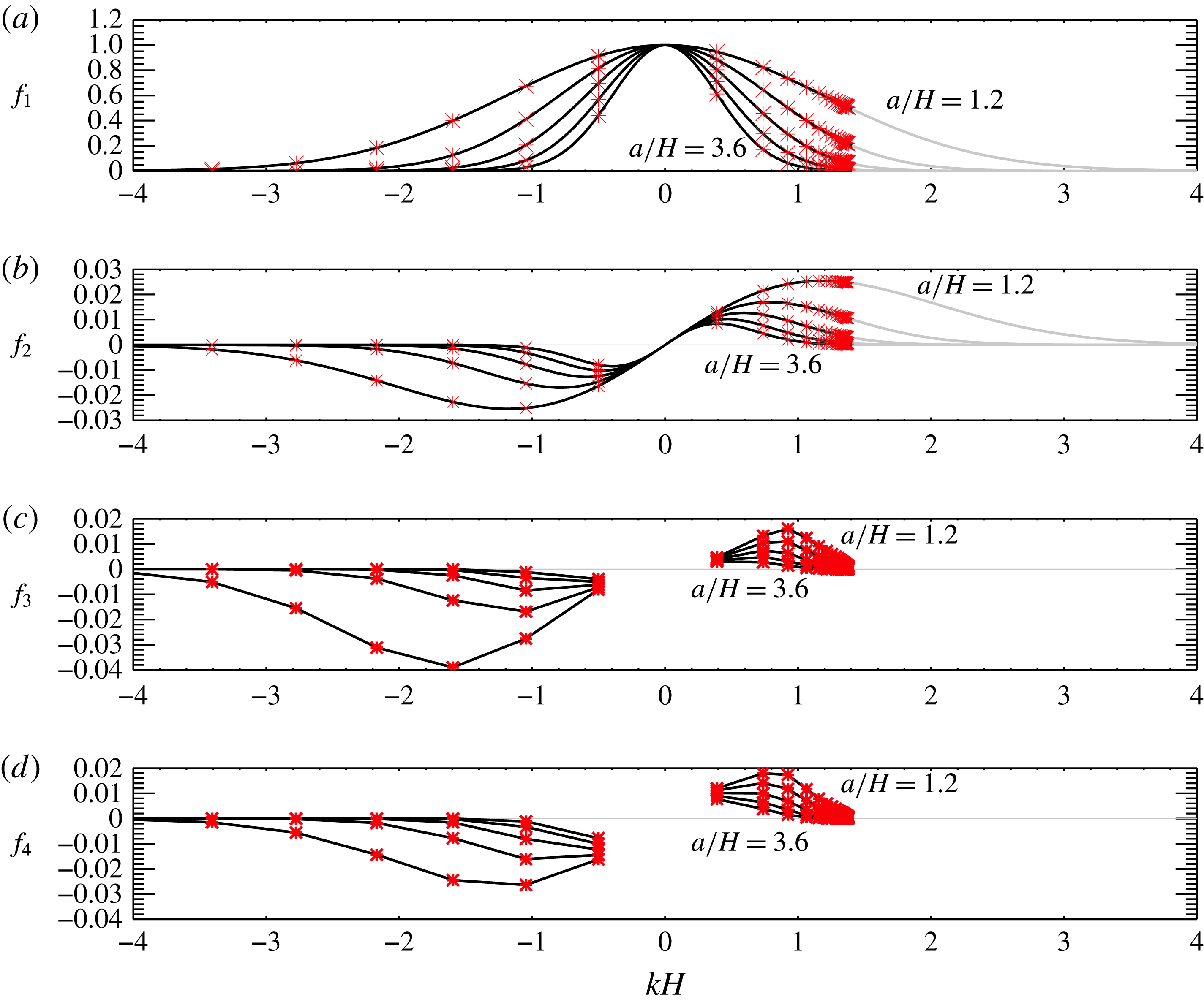
Figure 7. Partial coefficients in expressions for theoretical values for
 $u_{ds}$
and
$u_{ds}$
and
 $w_{ds}$
for waves of tidal frequency (
$w_{ds}$
for waves of tidal frequency (
 $n=1$
). (a)
$n=1$
). (a)
 $f_{1}={\hat{h}}(k)/{\hat{h}}(0)$
for the Gaussian ridge. Curves are for
$f_{1}={\hat{h}}(k)/{\hat{h}}(0)$
for the Gaussian ridge. Curves are for
 $a/H=1.2$
, 1.8, 2.4, 3.0 and 3.6. Red stars show the discrete spectrum for background current (2.4) for
$a/H=1.2$
, 1.8, 2.4, 3.0 and 3.6. Red stars show the discrete spectrum for background current (2.4) for
 $U_{s}/(NH)=0.1$
,
$U_{s}/(NH)=0.1$
,
 $d_{s}/H=0.08$
and
$d_{s}/H=0.08$
and
 $z_{s}/H=-0.3$
. (b)
$z_{s}/H=-0.3$
. (b)
 $f_{2}=({\hat{h}}(k)/{\hat{h}}(0))\text{J}_{1}(-kU_{0}/\unicode[STIX]{x1D714}_{0})$
. (c)
$f_{2}=({\hat{h}}(k)/{\hat{h}}(0))\text{J}_{1}(-kU_{0}/\unicode[STIX]{x1D714}_{0})$
. (c)
 $f_{3}=({\hat{h}}(k)/{\hat{h}}(0))\text{J}_{1}(-kU_{0}/\unicode[STIX]{x1D714}_{0})/|\unicode[STIX]{x2202}\unicode[STIX]{x1D719}_{1}/\unicode[STIX]{x2202}k|$
. (d)
$f_{3}=({\hat{h}}(k)/{\hat{h}}(0))\text{J}_{1}(-kU_{0}/\unicode[STIX]{x1D714}_{0})/|\unicode[STIX]{x2202}\unicode[STIX]{x1D719}_{1}/\unicode[STIX]{x2202}k|$
. (d)
 $f_{4}=({\hat{h}}(k)/{\hat{h}}(0))\text{J}_{1}(-kU_{0}/\unicode[STIX]{x1D714}_{0})/|\unicode[STIX]{x2202}\unicode[STIX]{x1D719}_{1}/\unicode[STIX]{x2202}k|k$
. In panels (c,d) values shown are for
$f_{4}=({\hat{h}}(k)/{\hat{h}}(0))\text{J}_{1}(-kU_{0}/\unicode[STIX]{x1D714}_{0})/|\unicode[STIX]{x2202}\unicode[STIX]{x1D719}_{1}/\unicode[STIX]{x2202}k|k$
. In panels (c,d) values shown are for
 $k_{1m}^{\pm }$
. In panels (a,b) black curves show range of
$k_{1m}^{\pm }$
. In panels (a,b) black curves show range of
 $k$
values to which the discrete spectrum belong; grey shows the range of the continuous spectrum.
$k$
values to which the discrete spectrum belong; grey shows the range of the continuous spectrum.
In terms of this perturbation expansion the work term, away from the ridge, is
 $$\begin{eqnarray}W=\int _{-H}^{0}up_{d}\,\text{d}z=\unicode[STIX]{x1D716}\int _{-H}^{0}\bar{U}(z)p^{(0)}\,\text{d}z+\unicode[STIX]{x1D716}^{2}\int _{-H}^{0}(\bar{U}(z)p^{(1)}+u^{(0)}p^{(0)})\,\text{d}z+O(\unicode[STIX]{x1D716}^{3}).\end{eqnarray}$$
Using
 $\langle \cdot \rangle$
to denote tidally averaged values, we have
$\langle \cdot \rangle$
to denote tidally averaged values, we have
 $$\begin{eqnarray}\langle W\rangle =\unicode[STIX]{x1D716}^{2}\int _{-H}^{0}(\bar{U}(z)\langle p^{(1)}\rangle +\langle u^{(0)}p^{(0)}\rangle )\,\text{d}z+O(\unicode[STIX]{x1D716}^{3})\end{eqnarray}$$
since the mean of
 $p^{(0)}$
is zero. Similarly, the tidally averaged kinetic energy flux is
$p^{(0)}$
is zero. Similarly, the tidally averaged kinetic energy flux is
 $$\begin{eqnarray}\langle KE_{f}\rangle =\unicode[STIX]{x1D716}^{2}\int _{-H}^{0}\left(\frac{3}{2}\bar{U}^{2}(z)\langle u^{(1)}\rangle +\frac{1}{2}\bar{U}(z)\langle 3(u^{(0)})^{2}+(w^{(0)})^{2}\rangle \right)\,\text{d}z+O(\unicode[STIX]{x1D716}^{3}),\end{eqnarray}$$
and the available potential energy flux is
 $$\begin{eqnarray}\langle APE_{f}\rangle =\int _{-H}^{0}\bar{U}(z)\langle E_{a}\rangle \,\text{d}z=\unicode[STIX]{x1D716}^{2}\int _{-H}^{0}\frac{g^{2}}{2N^{2}}\bar{U}(z)\langle (\unicode[STIX]{x1D70C}^{(0)})^{2}\rangle \,\text{d}z+O(\unicode[STIX]{x1D716}^{3}).\end{eqnarray}$$
For
 $\bar{U}(z)\neq 0$
the leading-order mean kinetic and available potential energy fluxes are of the same order as the work term and the mean second-order pressure and horizontal currents contribute to the leading-order terms.
$\bar{U}(z)\neq 0$
the leading-order mean kinetic and available potential energy fluxes are of the same order as the work term and the mean second-order pressure and horizontal currents contribute to the leading-order terms.
Because the second and higher harmonics are very small in our simulations in the following we assume all first-order terms are of tidal frequency. From linear theory we can calculate
 $$\begin{eqnarray}\langle W\rangle _{lin}=\int _{-H}^{0}\langle u^{(0)}p^{(0)}\rangle \,\text{d}z=\mathop{\sum }_{i=1}^{M}\mathop{\sum }_{j=1}^{M}\int _{-H}^{0}\langle u_{i}p_{j}\rangle \,\text{d}z,\end{eqnarray}$$
where
 $M$
is the number of modes included and
$M$
is the number of modes included and
 $u_{i}$
and
$u_{i}$
and
 $p_{i}$
are the contributions of mode-
$p_{i}$
are the contributions of mode-
 $i$
to
$i$
to
 $u^{(0)}$
and
$u^{(0)}$
and
 $p^{(0)}$
. Let
$p^{(0)}$
. Let
 $$\begin{eqnarray}W_{ij}^{l}=\int _{-H}^{0}\langle u_{i}p_{j}\rangle \,\text{d}z,\end{eqnarray}$$
with the superscript
 $l$
denoting linear theory. From (4.21) and (4.23), using the fact that
$l$
denoting linear theory. From (4.21) and (4.23), using the fact that
 ${\hat{h}}$
is real for our symmetric Gaussian ridge, let
${\hat{h}}$
is real for our symmetric Gaussian ridge, let
 $$\begin{eqnarray}u_{i}=A_{i}\sin (\unicode[STIX]{x1D703}_{i}(x,t))\unicode[STIX]{x1D719}_{i}^{\prime }(z),\end{eqnarray}$$
where
 $\unicode[STIX]{x1D703}_{i}(x,t)=k_{i}x-\unicode[STIX]{x1D714}_{0}t$
for all
$\unicode[STIX]{x1D703}_{i}(x,t)=k_{i}x-\unicode[STIX]{x1D714}_{0}t$
for all
 $i$
since the modes are in phase at
$i$
since the modes are in phase at
 $x=t=0$
. Then incompressibility gives
$x=t=0$
. Then incompressibility gives
 $$\begin{eqnarray}w_{i}=-k_{i}A_{i}\cos (\unicode[STIX]{x1D703}_{i})\unicode[STIX]{x1D719}_{i}(z)\end{eqnarray}$$
and from the horizontal momentum equation
 $$\begin{eqnarray}p_{i}=\frac{A_{i}}{k_{i}}\sin (\unicode[STIX]{x1D703}_{i})[(c_{i}-\bar{U})\unicode[STIX]{x1D719}_{i}^{\prime }+\bar{U}^{\prime }(z)\unicode[STIX]{x1D719}_{i}(z)]\end{eqnarray}$$
hence
 $$\begin{eqnarray}u_{i}p_{j}=\frac{A_{i}A_{j}}{2k_{j}}[\cos (\unicode[STIX]{x1D703}_{i}-\unicode[STIX]{x1D703}_{j})-\cos (\unicode[STIX]{x1D703}_{i}+\unicode[STIX]{x1D703}_{j})][(c_{j}-\bar{U})\unicode[STIX]{x1D719}_{j}^{\prime }+\bar{U}^{\prime }(z)\unicode[STIX]{x1D719}_{j}(z)]\unicode[STIX]{x1D719}_{i}^{\prime }(z).\end{eqnarray}$$
Taking the time average we obtain
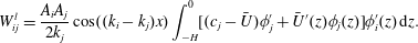 $$\begin{eqnarray}W_{ij}^{l}=\frac{A_{i}A_{j}}{2k_{j}}\cos ((k_{i}-k_{j})x)\int _{-H}^{0}[(c_{j}-\bar{U})\unicode[STIX]{x1D719}_{j}^{\prime }+\bar{U}^{\prime }(z)\unicode[STIX]{x1D719}_{j}(z)]\unicode[STIX]{x1D719}_{i}^{\prime }(z)\,\text{d}z.\end{eqnarray}$$
In the absence of a background current
 $W_{ij}^{l}=0$
for
$W_{ij}^{l}=0$
for
 $i\neq j$
because the eigenmodes
$i\neq j$
because the eigenmodes
 $\unicode[STIX]{x1D719}_{i}^{\prime }$
are orthogonal for waves of a fixed frequency but in general this is not the case. Hence the cross-terms
$\unicode[STIX]{x1D719}_{i}^{\prime }$
are orthogonal for waves of a fixed frequency but in general this is not the case. Hence the cross-terms
 $W_{ij}^{l}$
for
$W_{ij}^{l}$
for
 $i\neq j$
make a spatially varying contribution to the energy flux.
$i\neq j$
make a spatially varying contribution to the energy flux.
Similarly, the leading-order contribution to the kinetic energy flux from the leading-order velocity perturbation is
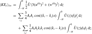 $$\begin{eqnarray}\displaystyle \langle KE_{f}\rangle _{lin} & = & \displaystyle \int _{-H}^{0}\frac{1}{2}\bar{U}\langle 3(u^{(0)})^{2}+(w^{(0)})^{2}\rangle \,\text{d}z\nonumber\\ \displaystyle & = & \displaystyle \mathop{\sum }_{i,j}\frac{3}{4}A_{i}A_{j}\cos ((k_{i}-k_{j})x)\int _{-H}^{0}\bar{U}(z)\unicode[STIX]{x1D719}_{i}^{\prime }\unicode[STIX]{x1D719}_{j}^{\prime }\,\text{d}z\nonumber\\ \displaystyle & & \displaystyle +\,\mathop{\sum }_{i,j}\frac{1}{4}A_{i}A_{j}k_{i}k_{j}\cos ((k_{i}-k_{j})x)\int _{-H}^{0}\bar{U}(z)\unicode[STIX]{x1D719}_{i}\unicode[STIX]{x1D719}_{j}\,\text{d}z.\end{eqnarray}$$
The second term, which is the flux of vertical kinetic energy, is negligible in our simulations. Let
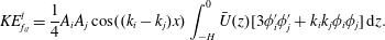 $$\begin{eqnarray}KE_{f_{ij}}^{l}=\frac{1}{4}A_{i}A_{j}\cos ((k_{i}-k_{j})x)\int _{-H}^{0}\bar{U}(z)[3\unicode[STIX]{x1D719}_{i}^{\prime }\unicode[STIX]{x1D719}_{j}^{\prime }+k_{i}k_{j}\unicode[STIX]{x1D719}_{i}\unicode[STIX]{x1D719}_{j}]\,\text{d}z.\end{eqnarray}$$
As for the work term, the cross-terms with
 $i\neq j$
are generally non-zero. The linearized density equation gives
$i\neq j$
are generally non-zero. The linearized density equation gives
 $$\begin{eqnarray}\unicode[STIX]{x1D70C}_{i}=\frac{A_{i}}{g}\sin \unicode[STIX]{x1D703}_{i}\frac{N^{2}}{c_{i}-\bar{U}}\unicode[STIX]{x1D719}_{i},\end{eqnarray}$$
the leading-order contribution to the available potential energy flux is
 $$\begin{eqnarray}\langle APE_{f}\rangle _{lin}=\mathop{\sum }_{i,j}APE_{f_{ij}}^{l},\end{eqnarray}$$
where
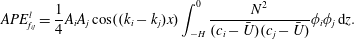 $$\begin{eqnarray}APE_{f_{ij}}^{l}=\frac{1}{4}A_{i}A_{j}\cos ((k_{i}-k_{j})x)\int _{-H}^{0}\frac{N^{2}}{(c_{i}-\bar{U})(c_{j}-\bar{U})}\unicode[STIX]{x1D719}_{i}\unicode[STIX]{x1D719}_{j}\,\text{d}z.\end{eqnarray}$$
Figure 8 shows the accumulated percentage of the total linear energy flux contributed by the squared terms as a function of the number of modes, i.e.
 $\sum _{i=1}^{M}E_{f_{i}}^{l}$
where
$\sum _{i=1}^{M}E_{f_{i}}^{l}$
where
 $E_{f_{i}}^{l}=W_{ii}^{l}+KE_{f_{ii}}^{l}+APE_{f_{ii}}^{l}$
. Only the squared terms with
$E_{f_{i}}^{l}=W_{ii}^{l}+KE_{f_{ii}}^{l}+APE_{f_{ii}}^{l}$
. Only the squared terms with
 $i=j$
are included because the cross-terms vary with
$i=j$
are included because the cross-terms vary with
 $x$
with average values of zero. More modes are needed to estimate the total energy flux for the downstream (rightward) propagating waves than for the upstream (leftward) propagating waves and the narrower the ridge the more modes are needed. As we will see below, the linear theory does not accurately predict the energy flux for narrow ridges.
$x$
with average values of zero. More modes are needed to estimate the total energy flux for the downstream (rightward) propagating waves than for the upstream (leftward) propagating waves and the narrower the ridge the more modes are needed. As we will see below, the linear theory does not accurately predict the energy flux for narrow ridges.
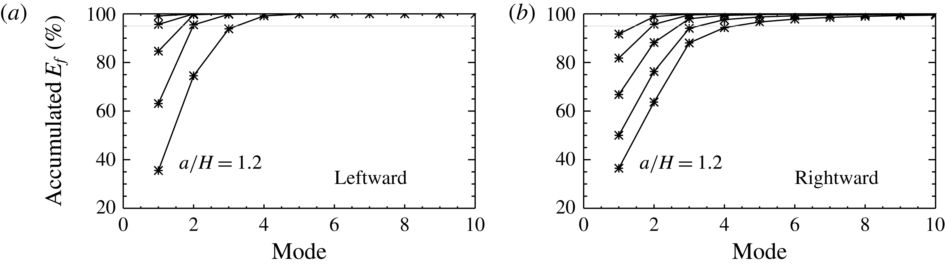
Figure 8. Accumulated percentage of total linear energy flux
 $100\times \sum _{j=1}^{n_{m}}E_{f_{j}}^{l}/\sum _{j=1}^{16}E_{f_{j}}^{l}$
versus number of modes
$100\times \sum _{j=1}^{n_{m}}E_{f_{j}}^{l}/\sum _{j=1}^{16}E_{f_{j}}^{l}$
versus number of modes
 $n_{m}$
. (a) Leftward propagating waves. (b) Rightward propagating waves. Results are shown for
$n_{m}$
. (a) Leftward propagating waves. (b) Rightward propagating waves. Results are shown for
 $a/H=1.2$
,
$a/H=1.2$
,
 $1.8$
,
$1.8$
,
 $2.4$
,
$2.4$
,
 $3.0$
and
$3.0$
and
 $3.6$
. As
$3.6$
. As
 $a/H$
increases the fraction of the total energy flux in the first mode increases.
$a/H$
increases the fraction of the total energy flux in the first mode increases.
5 Validation tests
Validation tests were done by checking convergence and how well the energy balance equation (3.17) is satisfied. Here we present results for the ridge with
 $a/H=1.8$
from set 4. The minimum Richardson number is
$a/H=1.8$
from set 4. The minimum Richardson number is
 $1.8$
and the slope is sub-critical with
$1.8$
and the slope is sub-critical with
 $\unicode[STIX]{x1D6FE}=0.34$
.
$\unicode[STIX]{x1D6FE}=0.34$
.
Simulations done with horizontal resolutions of
 $\unicode[STIX]{x0394}x/H=0.02$
and
$\unicode[STIX]{x0394}x/H=0.02$
and
 $0.01$
and time steps of
$0.01$
and time steps of
 $N\unicode[STIX]{x0394}t=0.069$
and
$N\unicode[STIX]{x0394}t=0.069$
and
 $0.0345$
showed that
$0.0345$
showed that
 $\unicode[STIX]{x0394}x/H=0.02$
and
$\unicode[STIX]{x0394}x/H=0.02$
and
 $N\unicode[STIX]{x0394}t=0.069$
were generally adequate. For the strongest current we use
$N\unicode[STIX]{x0394}t=0.069$
were generally adequate. For the strongest current we use
 $N\unicode[STIX]{x0394}t=0.0345$
. A uniform vertical grid spacing with 250 grid cells was used, 400 grid cells giving similar results. This gives a vertical resolution of
$N\unicode[STIX]{x0394}t=0.0345$
. A uniform vertical grid spacing with 250 grid cells was used, 400 grid cells giving similar results. This gives a vertical resolution of
 $\unicode[STIX]{x0394}z/H=0.004$
in the deep water.
$\unicode[STIX]{x0394}z/H=0.004$
in the deep water.
Figure 9 compares terms in the energy balance equation (3.17) for a Lagrangian region spanning the ridge. The dominant balance is between
 $\text{d}\bar{E}/\text{d}t$
and
$\text{d}\bar{E}/\text{d}t$
and
 $W|_{\unicode[STIX]{x1D709}_{l}}^{\unicode[STIX]{x1D709}_{r}}$
(figure 9
a). A major contribution to the energy
$W|_{\unicode[STIX]{x1D709}_{l}}^{\unicode[STIX]{x1D709}_{r}}$
(figure 9
a). A major contribution to the energy
 $\bar{E}$
is associated with the time varying barotropic currents over the ridge. In conjunction there are large oscillating pressure gradients accelerating the barotropic currents. These form the dominant balance in the energetics over the ridge. Panel (b) shows that
$\bar{E}$
is associated with the time varying barotropic currents over the ridge. In conjunction there are large oscillating pressure gradients accelerating the barotropic currents. These form the dominant balance in the energetics over the ridge. Panel (b) shows that
 $\text{d}\bar{E}/\text{d}t-W|_{\unicode[STIX]{x1D709}_{l}}^{\unicode[STIX]{x1D709}_{r}}$
is largely balanced by
$\text{d}\bar{E}/\text{d}t-W|_{\unicode[STIX]{x1D709}_{l}}^{\unicode[STIX]{x1D709}_{r}}$
is largely balanced by
 $KE_{f}|_{\unicode[STIX]{x1D709}_{l}}^{\unicode[STIX]{x1D709}_{r}}$
. Panel (c) shows that
$KE_{f}|_{\unicode[STIX]{x1D709}_{l}}^{\unicode[STIX]{x1D709}_{r}}$
. Panel (c) shows that
 $\text{d}\bar{E}/\text{d}t-W|_{\unicode[STIX]{x1D709}_{l}}^{\unicode[STIX]{x1D709}_{r}}-KE_{f}|_{\unicode[STIX]{x1D709}_{l}}^{\unicode[STIX]{x1D709}_{r}}$
and the conversion term
$\text{d}\bar{E}/\text{d}t-W|_{\unicode[STIX]{x1D709}_{l}}^{\unicode[STIX]{x1D709}_{r}}-KE_{f}|_{\unicode[STIX]{x1D709}_{l}}^{\unicode[STIX]{x1D709}_{r}}$
and the conversion term
 $G$
are virtually identical. Panel (d) shows the sum of all the terms
$G$
are virtually identical. Panel (d) shows the sum of all the terms
 $\text{d}\bar{E}/\text{d}t-W|_{\unicode[STIX]{x1D709}_{l}}^{\unicode[STIX]{x1D709}_{r}}-KE_{f}|_{\unicode[STIX]{x1D709}_{l}}^{\unicode[STIX]{x1D709}_{r}}-APE_{f}|_{\unicode[STIX]{x1D709}_{l}}^{\unicode[STIX]{x1D709}_{r}}-G$
which should theoretically be equal to zero. Peak values are approximately 0.016 compared with peak values of approximately 60 for
$\text{d}\bar{E}/\text{d}t-W|_{\unicode[STIX]{x1D709}_{l}}^{\unicode[STIX]{x1D709}_{r}}-KE_{f}|_{\unicode[STIX]{x1D709}_{l}}^{\unicode[STIX]{x1D709}_{r}}-APE_{f}|_{\unicode[STIX]{x1D709}_{l}}^{\unicode[STIX]{x1D709}_{r}}-G$
which should theoretically be equal to zero. Peak values are approximately 0.016 compared with peak values of approximately 60 for
 $\text{d}\bar{E}/\text{d}t$
so the energy budget is satisfied to within approximately 0.025 %.
$\text{d}\bar{E}/\text{d}t$
so the energy budget is satisfied to within approximately 0.025 %.
The energy balance in a Lagrangian domain to the right of the ridge was also analysed using flux lines with mean positions of
 $5.4$
and
$5.4$
and
 $9.4$
(not shown). The length of this region is 25 % of the wavelength of a rightward mode-one tidal frequency wave. Off the ridge the conversion term is zero and the energy fluctuations are not affected by flow constriction over the ridge. The dominant balance is between
$9.4$
(not shown). The length of this region is 25 % of the wavelength of a rightward mode-one tidal frequency wave. Off the ridge the conversion term is zero and the energy fluctuations are not affected by flow constriction over the ridge. The dominant balance is between
 $\text{d}\bar{E}/\text{d}t$
,
$\text{d}\bar{E}/\text{d}t$
,
 $W|_{\unicode[STIX]{x1D709}_{r}}^{\unicode[STIX]{x1D709}_{l}}$
and
$W|_{\unicode[STIX]{x1D709}_{r}}^{\unicode[STIX]{x1D709}_{l}}$
and
 $KE_{f}|_{\unicode[STIX]{x1D709}_{r}}^{\unicode[STIX]{x1D709}_{l}}$
, with the latter two approximately half the size of
$KE_{f}|_{\unicode[STIX]{x1D709}_{r}}^{\unicode[STIX]{x1D709}_{l}}$
, with the latter two approximately half the size of
 $\text{d}\bar{E}/\text{d}t$
. Peak values of the net balance
$\text{d}\bar{E}/\text{d}t$
. Peak values of the net balance
 $\text{d}\bar{E}/\text{d}t-W|_{\unicode[STIX]{x1D709}_{r}}^{\unicode[STIX]{x1D709}_{l}}-KE_{f}|_{\unicode[STIX]{x1D709}_{r}}^{\unicode[STIX]{x1D709}_{l}}-APE_{f}|_{\unicode[STIX]{x1D709}_{r}}^{\unicode[STIX]{x1D709}_{l}}$
are approximately 0.01, approximately 0.03 % of the peak values of
$\text{d}\bar{E}/\text{d}t-W|_{\unicode[STIX]{x1D709}_{r}}^{\unicode[STIX]{x1D709}_{l}}-KE_{f}|_{\unicode[STIX]{x1D709}_{r}}^{\unicode[STIX]{x1D709}_{l}}-APE_{f}|_{\unicode[STIX]{x1D709}_{r}}^{\unicode[STIX]{x1D709}_{l}}$
are approximately 0.01, approximately 0.03 % of the peak values of
 $\text{d}\bar{E}/\text{d}t$
so the energy budget in this off-ridge domain is also satisfied to high accuracy.
$\text{d}\bar{E}/\text{d}t$
so the energy budget in this off-ridge domain is also satisfied to high accuracy.
Figure 10 compares tidally averaged values in the off-ridge Lagrangian domain. Panel (a) shows the work terms and kinetic energy fluxes at the left and right boundaries. All undergo oscillations with a period of about
 $4T$
as well as longer period fluctuations. The net energy balance,
$4T$
as well as longer period fluctuations. The net energy balance,
 $\langle \text{d}\bar{E}/\text{d}t\rangle -\langle W\rangle |_{\unicode[STIX]{x1D709}_{r}}^{\unicode[STIX]{x1D709}_{l}}-\langle KE_{f}\rangle |_{\unicode[STIX]{x1D709}_{r}}^{\unicode[STIX]{x1D709}_{l}}-\langle APE_{f}\rangle |_{\unicode[STIX]{x1D709}_{r}}^{\unicode[STIX]{x1D709}_{l}}$
, has a typical value of about
$\langle \text{d}\bar{E}/\text{d}t\rangle -\langle W\rangle |_{\unicode[STIX]{x1D709}_{r}}^{\unicode[STIX]{x1D709}_{l}}-\langle KE_{f}\rangle |_{\unicode[STIX]{x1D709}_{r}}^{\unicode[STIX]{x1D709}_{l}}-\langle APE_{f}\rangle |_{\unicode[STIX]{x1D709}_{r}}^{\unicode[STIX]{x1D709}_{l}}$
, has a typical value of about
 $0.01$
(panel c) and does not undergo significant oscillations. This is approximately 0.5 % of a typical value for
$0.01$
(panel c) and does not undergo significant oscillations. This is approximately 0.5 % of a typical value for
 $\langle W\rangle |_{\unicode[STIX]{x1D709}_{l}}$
.
$\langle W\rangle |_{\unicode[STIX]{x1D709}_{l}}$
.

Figure 9. Energy balance in a Lagrangian domain spanning the ridge. Values non-dimensionalized by the flux scale
 $F_{0}$
. Time in tidal periods. The domain lies between flux lines with mean positions at
$F_{0}$
. Time in tidal periods. The domain lies between flux lines with mean positions at
 $x/H=\pm 5.4$
for a case with
$x/H=\pm 5.4$
for a case with
 $U_{s}/(NH)=0.1$
,
$U_{s}/(NH)=0.1$
,
 $h_{0}/H=0.1$
and
$h_{0}/H=0.1$
and
 $a/H=1.8$
. Resolution is
$a/H=1.8$
. Resolution is
 $\text{d}x/H=0.02$
in the horizontal with
$\text{d}x/H=0.02$
in the horizontal with
 $J=250$
. Time step
$J=250$
. Time step
 $N\unicode[STIX]{x0394}t=0.069$
. (a)
$N\unicode[STIX]{x0394}t=0.069$
. (a)
 $\text{d}\bar{E}/\text{d}t$
(solid),
$\text{d}\bar{E}/\text{d}t$
(solid),
 $W|_{\unicode[STIX]{x1D709}_{r}}^{\unicode[STIX]{x1D709}_{l}}$
(dash-dot),
$W|_{\unicode[STIX]{x1D709}_{r}}^{\unicode[STIX]{x1D709}_{l}}$
(dash-dot),
 $KE_{f}|_{\unicode[STIX]{x1D709}_{r}}^{\unicode[STIX]{x1D709}_{l}}$
(dash), conversion term
$KE_{f}|_{\unicode[STIX]{x1D709}_{r}}^{\unicode[STIX]{x1D709}_{l}}$
(dash), conversion term
 $G$
(dots). (b)
$G$
(dots). (b)
 $\text{d}\bar{E}/\text{d}t-W|_{\unicode[STIX]{x1D709}_{r}}^{\unicode[STIX]{x1D709}_{l}}$
(solid),
$\text{d}\bar{E}/\text{d}t-W|_{\unicode[STIX]{x1D709}_{r}}^{\unicode[STIX]{x1D709}_{l}}$
(solid),
 $KE_{f}|_{\unicode[STIX]{x1D709}_{r}}^{\unicode[STIX]{x1D709}_{l}}$
(dots),
$KE_{f}|_{\unicode[STIX]{x1D709}_{r}}^{\unicode[STIX]{x1D709}_{l}}$
(dots),
 $G$
(dashed),
$G$
(dashed),
 $APE_{f}|_{\unicode[STIX]{x1D709}_{r}}^{\unicode[STIX]{x1D709}_{l}}$
(dash-dots). The latter is indistinguishable from zero. (c)
$APE_{f}|_{\unicode[STIX]{x1D709}_{r}}^{\unicode[STIX]{x1D709}_{l}}$
(dash-dots). The latter is indistinguishable from zero. (c)
 $\text{d}\bar{E}/\text{d}t-W|_{\unicode[STIX]{x1D709}_{r}}^{\unicode[STIX]{x1D709}_{l}}-KE_{f}|_{\unicode[STIX]{x1D709}_{r}}^{\unicode[STIX]{x1D709}_{l}}$
(solid black),
$\text{d}\bar{E}/\text{d}t-W|_{\unicode[STIX]{x1D709}_{r}}^{\unicode[STIX]{x1D709}_{l}}-KE_{f}|_{\unicode[STIX]{x1D709}_{r}}^{\unicode[STIX]{x1D709}_{l}}$
(solid black),
 $G$
(dashed),
$G$
(dashed),
 $APE_{f}|_{\unicode[STIX]{x1D709}_{r}}^{\unicode[STIX]{x1D709}_{l}}$
(dots). The first two curves are barely distinguishable. (d) Net balance
$APE_{f}|_{\unicode[STIX]{x1D709}_{r}}^{\unicode[STIX]{x1D709}_{l}}$
(dots). The first two curves are barely distinguishable. (d) Net balance
 $\text{d}\bar{E}/\text{d}t-W|_{\unicode[STIX]{x1D709}_{r}}^{\unicode[STIX]{x1D709}_{l}}-G-KE_{f}|_{\unicode[STIX]{x1D709}_{r}}^{\unicode[STIX]{x1D709}_{l}}-APE_{f}|_{\unicode[STIX]{x1D709}_{r}}^{\unicode[STIX]{x1D709}_{l}}$
.
$\text{d}\bar{E}/\text{d}t-W|_{\unicode[STIX]{x1D709}_{r}}^{\unicode[STIX]{x1D709}_{l}}-G-KE_{f}|_{\unicode[STIX]{x1D709}_{r}}^{\unicode[STIX]{x1D709}_{l}}-APE_{f}|_{\unicode[STIX]{x1D709}_{r}}^{\unicode[STIX]{x1D709}_{l}}$
.

Figure 10. Energy balance in a Lagrangian domain off the ridge: tidal averages scaled by
 $F_{0}$
. The domain lies between flux lines with mean positions at
$F_{0}$
. The domain lies between flux lines with mean positions at
 $x/H=5.4$
and
$x/H=5.4$
and
 $9.4$
for the same case as in figure 9. (a)
$9.4$
for the same case as in figure 9. (a)
 $\langle W|_{\unicode[STIX]{x1D709}_{l}}\rangle$
(solid),
$\langle W|_{\unicode[STIX]{x1D709}_{l}}\rangle$
(solid),
 $\langle W|_{\unicode[STIX]{x1D709}_{r}}\rangle$
(dashed),
$\langle W|_{\unicode[STIX]{x1D709}_{r}}\rangle$
(dashed),
 $\langle KE_{f}|_{\unicode[STIX]{x1D709}_{l}}\rangle$
(dots) and
$\langle KE_{f}|_{\unicode[STIX]{x1D709}_{l}}\rangle$
(dots) and
 $\langle KE_{f}|_{\unicode[STIX]{x1D709}_{r}}\rangle$
(dash-dot). (b)
$\langle KE_{f}|_{\unicode[STIX]{x1D709}_{r}}\rangle$
(dash-dot). (b)
 $\langle \text{d}\bar{E}/\text{d}t\rangle$
(solid black),
$\langle \text{d}\bar{E}/\text{d}t\rangle$
(solid black),
 $\langle W|_{\unicode[STIX]{x1D709}_{r}}^{\unicode[STIX]{x1D709}_{l}}\rangle$
(dashed),
$\langle W|_{\unicode[STIX]{x1D709}_{r}}^{\unicode[STIX]{x1D709}_{l}}\rangle$
(dashed),
 $\langle KE_{f}|_{\unicode[STIX]{x1D709}_{r}}^{\unicode[STIX]{x1D709}_{l}}\rangle$
(dots),
$\langle KE_{f}|_{\unicode[STIX]{x1D709}_{r}}^{\unicode[STIX]{x1D709}_{l}}\rangle$
(dots),
 $\langle APE_{f}|_{\unicode[STIX]{x1D709}_{r}}^{\unicode[STIX]{x1D709}_{l}}\rangle$
(dash-dot). (c) Net energy flux:
$\langle APE_{f}|_{\unicode[STIX]{x1D709}_{r}}^{\unicode[STIX]{x1D709}_{l}}\rangle$
(dash-dot). (c) Net energy flux:
 $\langle \text{d}\bar{E}/\text{d}t\rangle -\langle W|_{\unicode[STIX]{x1D709}_{r}}^{\unicode[STIX]{x1D709}_{l}}\rangle -\langle KE_{f}|_{\unicode[STIX]{x1D709}_{r}}^{\unicode[STIX]{x1D709}_{l}}\rangle -\langle APE_{f}|_{\unicode[STIX]{x1D709}_{r}}^{\unicode[STIX]{x1D709}_{l}}\rangle$
(solid);
$\langle \text{d}\bar{E}/\text{d}t\rangle -\langle W|_{\unicode[STIX]{x1D709}_{r}}^{\unicode[STIX]{x1D709}_{l}}\rangle -\langle KE_{f}|_{\unicode[STIX]{x1D709}_{r}}^{\unicode[STIX]{x1D709}_{l}}\rangle -\langle APE_{f}|_{\unicode[STIX]{x1D709}_{r}}^{\unicode[STIX]{x1D709}_{l}}\rangle$
(solid);
 $\langle \text{d}\bar{E}/\text{d}t\rangle -\langle W|_{\unicode[STIX]{x1D709}_{r}}^{\unicode[STIX]{x1D709}_{l}}\rangle -\langle KE_{f}|_{\unicode[STIX]{x1D709}_{r}}^{\unicode[STIX]{x1D709}_{l}}\rangle$
(dots),
$\langle \text{d}\bar{E}/\text{d}t\rangle -\langle W|_{\unicode[STIX]{x1D709}_{r}}^{\unicode[STIX]{x1D709}_{l}}\rangle -\langle KE_{f}|_{\unicode[STIX]{x1D709}_{r}}^{\unicode[STIX]{x1D709}_{l}}\rangle$
(dots),
 $\langle APE_{f}|_{\unicode[STIX]{x1D709}_{r}}^{\unicode[STIX]{x1D709}_{l}}\rangle$
(dash-dot).
$\langle APE_{f}|_{\unicode[STIX]{x1D709}_{r}}^{\unicode[STIX]{x1D709}_{l}}\rangle$
(dash-dot).
6 Results
Total energy fluxes averaged over one tidal period have temporal fluctuations with amplitudes of up to 10 % of their mean values. Averaging over four periods significantly reduced these variations so henceforth we use four period averages, i.e. we now define the averaging operator as
 $$\begin{eqnarray}\langle \cdot \rangle (t)=\frac{1}{4T}\int _{t-4T}^{t}\cdot \,\text{d}t.\end{eqnarray}$$
Most simulations were limited to twenty periods and we will generally report results at this time. Some sets were run for forty tidal periods.
Figure 11 shows the total energy flux
 $\langle E_{f}\rangle$
and the contributions from
$\langle E_{f}\rangle$
and the contributions from
 $\langle W\rangle$
,
$\langle W\rangle$
,
 $\langle KE_{f}\rangle$
and
$\langle KE_{f}\rangle$
and
 $\langle APE_{f}\rangle$
, as a function of distance from the ridge for the cases from set 4 with
$\langle APE_{f}\rangle$
, as a function of distance from the ridge for the cases from set 4 with
 $a/H=1.8$
(a,b) and
$a/H=1.8$
(a,b) and
 $a/H=6$
(c,d). The former is the case depicted in figure 2. Values at
$a/H=6$
(c,d). The former is the case depicted in figure 2. Values at
 $t=20T$
(symbols) and
$t=20T$
(symbols) and
 $40T$
(grey curves) are shown. Note the much larger range of flux values used for the left side of the narrow ridge (panel a).
$40T$
(grey curves) are shown. Note the much larger range of flux values used for the left side of the narrow ridge (panel a).
Figure 11. Tidally averaged energy fluxes at
 $t=20T$
and
$t=20T$
and
 $40T$
(averaged over previous four periods) scaled by
$40T$
(averaged over previous four periods) scaled by
 $F_{0}$
as a function of distance for the cases from set 4 with
$F_{0}$
as a function of distance for the cases from set 4 with
 $a/H=1.8$
(a,b) and
$a/H=1.8$
(a,b) and
 $a/H=6$
(c,d). (a,c) Fluxes to left of ridge. (b,d) Fluxes to right of ridge. Note the much larger range of flux values in panel (a). Shown in each panel are the work term
$a/H=6$
(c,d). (a,c) Fluxes to left of ridge. (b,d) Fluxes to right of ridge. Note the much larger range of flux values in panel (a). Shown in each panel are the work term
 $\langle W\rangle$
(red), the total kinetic energy flux
$\langle W\rangle$
(red), the total kinetic energy flux
 $\langle KE_{f}\rangle$
(green), the available potential energy flux
$\langle KE_{f}\rangle$
(green), the available potential energy flux
 $\langle APE_{f}\rangle$
(blue) and the total energy flux
$\langle APE_{f}\rangle$
(blue) and the total energy flux
 $\langle E_{f}\rangle$
(black). For comparison the grey curves show the fluxes at
$\langle E_{f}\rangle$
(black). For comparison the grey curves show the fluxes at
 $t=40T$
.
$t=40T$
.

Figure 12. Comparison of theory and simulation results for
 $a/H=1.8$
from set 4 (same case depicted in figure 11
a,b). Shown are tidally averaged contributions to the energy fluxes at
$a/H=1.8$
from set 4 (same case depicted in figure 11
a,b). Shown are tidally averaged contributions to the energy fluxes at
 $t=40T$
scaled by
$t=40T$
scaled by
 $F_{0}$
as a function of distance. Panels (a,c,e) show values to the left of the ridge. Panels (b,d,f) show values to the right of the ridge. (a,b) Contributions to the work term:
$F_{0}$
as a function of distance. Panels (a,c,e) show values to the left of the ridge. Panels (b,d,f) show values to the right of the ridge. (a,b) Contributions to the work term:
 $\langle W_{1}\rangle$
(blue diamonds) and
$\langle W_{1}\rangle$
(blue diamonds) and
 $\langle W_{2}\rangle$
(red squares). The dashed black line shows
$\langle W_{2}\rangle$
(red squares). The dashed black line shows
 $\langle W\rangle _{lin}$
, the theoretical work term from first-order theory. (c,d)
$\langle W\rangle _{lin}$
, the theoretical work term from first-order theory. (c,d)
 $\langle KE_{f1}\rangle$
(green),
$\langle KE_{f1}\rangle$
(green),
 $\langle KE_{f2}\rangle$
(red) and
$\langle KE_{f2}\rangle$
(red) and
 $\langle APE_{f}\rangle$
(blue). The dashed and dotted lines show the theoretical kinetic energy flux
$\langle APE_{f}\rangle$
(blue). The dashed and dotted lines show the theoretical kinetic energy flux
 $\langle KE_{f}\rangle _{lin}$
and available potential energy flux
$\langle KE_{f}\rangle _{lin}$
and available potential energy flux
 $\langle APE_{f}\rangle _{lin}$
. (e,f) The total energy flux
$\langle APE_{f}\rangle _{lin}$
. (e,f) The total energy flux
 $\langle E_{f}\rangle$
from simulations (blue), contributions to the total energy flux that are second-order in the perturbation fields,
$\langle E_{f}\rangle$
from simulations (blue), contributions to the total energy flux that are second-order in the perturbation fields,
 $\langle W_{2}+KE_{f2}+APE_{f}\rangle$
(red) and the total theoretical energy flux
$\langle W_{2}+KE_{f2}+APE_{f}\rangle$
(red) and the total theoretical energy flux
 $\langle W+KE_{f}+APE_{f}\rangle _{lin}$
(black, dashed).
$\langle W+KE_{f}+APE_{f}\rangle _{lin}$
(black, dashed).
To the left of the narrower ridge the work term
 $\langle W\rangle$
and kinetic energy flux
$\langle W\rangle$
and kinetic energy flux
 $\langle KE_{f}\rangle$
, which have opposite signs, undergo large spatial fluctuations with a period
$\langle KE_{f}\rangle$
, which have opposite signs, undergo large spatial fluctuations with a period
 $x/H\approx 11.3$
(figure 11
a). Peak values of the magnitudes of
$x/H\approx 11.3$
(figure 11
a). Peak values of the magnitudes of
 $\langle KE_{f}\rangle$
and
$\langle KE_{f}\rangle$
and
 $\langle W\rangle$
occur at the locations where the beams reflect off the surface (see figures 1
a and 2). The fluctuation period is close to
$\langle W\rangle$
occur at the locations where the beams reflect off the surface (see figures 1
a and 2). The fluctuation period is close to
 $2\unicode[STIX]{x03C0}/H(k_{2}-k_{1})=11.5$
, the wavelength associated with the interaction of mode-one and mode-two waves (the mode-one wavelength is 12.5). The locations of the minimum and maximum values are independent of time (not shown) with values undergoing relatively small temporal oscillations. To the left of the ridge the kinetic energy flux is positive, i.e. it is in the direction opposite to that of wave propagation. The total mean energy flux
$2\unicode[STIX]{x03C0}/H(k_{2}-k_{1})=11.5$
, the wavelength associated with the interaction of mode-one and mode-two waves (the mode-one wavelength is 12.5). The locations of the minimum and maximum values are independent of time (not shown) with values undergoing relatively small temporal oscillations. To the left of the ridge the kinetic energy flux is positive, i.e. it is in the direction opposite to that of wave propagation. The total mean energy flux
 $\langle E_{f}\rangle$
is almost constant within a distance
$\langle E_{f}\rangle$
is almost constant within a distance
 $x/H$
of 40 from the ridge where the variations in
$x/H$
of 40 from the ridge where the variations in
 $\langle W\rangle$
are almost completely balanced by variations in
$\langle W\rangle$
are almost completely balanced by variations in
 $\langle KE_{f}\rangle$
. At larger distances from the ridge
$\langle KE_{f}\rangle$
. At larger distances from the ridge
 $\langle E_{f}\rangle$
has small spatial variations which grow with distance from the ridge. This appears to occur because the mean wave field beyond
$\langle E_{f}\rangle$
has small spatial variations which grow with distance from the ridge. This appears to occur because the mean wave field beyond
 $x/H=-30$
is still in a transient state as indicated by the averaged energy flux after 40 tidal periods (grey curve). At
$x/H=-30$
is still in a transient state as indicated by the averaged energy flux after 40 tidal periods (grey curve). At
 $t=20T$
linear theory predicts that the first 10 modes have reached
$t=20T$
linear theory predicts that the first 10 modes have reached
 $x/H=-30$
while only the first 5 have reached
$x/H=-30$
while only the first 5 have reached
 $x/H=-50$
.
$x/H=-50$
.
The fluxes to the right of the narrow ridge (figure 11
b) undergo significantly smaller spatial variations on much longer length scales. Variations in
 $\langle W\rangle$
are significant and are again largely balanced by variations in
$\langle W\rangle$
are significant and are again largely balanced by variations in
 $\langle KE_{f}\rangle$
. Their pattern is very different to that on the left side of the ridge.
$\langle KE_{f}\rangle$
. Their pattern is very different to that on the left side of the ridge.
 $\langle KE_{f}\rangle$
is again in the direction of wave propagation. For both the leftward and rightward propagating waves it is in the direction of the background current as the dominant contribution is from the
$\langle KE_{f}\rangle$
is again in the direction of wave propagation. For both the leftward and rightward propagating waves it is in the direction of the background current as the dominant contribution is from the
 $\bar{U}u^{2}$
term (see below). The total energy flux at
$\bar{U}u^{2}$
term (see below). The total energy flux at
 $t=20T$
is almost constant out to
$t=20T$
is almost constant out to
 $x/H=54$
due to the larger downstream group velocities (note different scales used for fluxes to the left and right of the ridge: the oscillations far to the left of the ridge are much larger than those far to the right of the ridge). The different patterns in
$x/H=54$
due to the larger downstream group velocities (note different scales used for fluxes to the left and right of the ridge: the oscillations far to the left of the ridge are much larger than those far to the right of the ridge). The different patterns in
 $\langle W\rangle$
and
$\langle W\rangle$
and
 $\langle KE_{f}\rangle$
to the left and right of the ridge is connected to the different patterns in the mean wave field (see figure 2).
$\langle KE_{f}\rangle$
to the left and right of the ridge is connected to the different patterns in the mean wave field (see figure 2).
Figure 12 shows a breakdown of
 $\langle W\rangle$
and
$\langle W\rangle$
and
 $\langle KE_{f}\rangle$
into their linear and quadratic parts (see (3.23) and (3.24)) for the narrower ridge (
$\langle KE_{f}\rangle$
into their linear and quadratic parts (see (3.23) and (3.24)) for the narrower ridge (
 $a/H=1.8$
). The fluxes predicted by first-order linear theory are also shown and they compare well with the second-order contributions. In particular, the linear first-order cross-terms, i.e.
$a/H=1.8$
). The fluxes predicted by first-order linear theory are also shown and they compare well with the second-order contributions. In particular, the linear first-order cross-terms, i.e.
 $W_{ij}^{l}$
,
$W_{ij}^{l}$
,
 $KE_{f_{ij}}^{l}$
and
$KE_{f_{ij}}^{l}$
and
 $APE_{f_{ij}}^{l}$
with
$APE_{f_{ij}}^{l}$
with
 $i\neq j$
, account for the spatial variations in the fluxes in the numerical simulations. The fluxes that are linear in the perturbation fields,
$i\neq j$
, account for the spatial variations in the fluxes in the numerical simulations. The fluxes that are linear in the perturbation fields,
 $\langle W_{1}\rangle$
and
$\langle W_{1}\rangle$
and
 $\langle KE_{f1}\rangle$
, make important contributions to the total flux, i.e. the second-order mean wave fields are important. Panels (e,f) show the total energy flux, the total second-order flux
$\langle KE_{f1}\rangle$
, make important contributions to the total flux, i.e. the second-order mean wave fields are important. Panels (e,f) show the total energy flux, the total second-order flux
 $\langle W_{2}+KE_{f2}+APE_{f}\rangle$
, and the total energy flux from linear theory. The latter two are very similar. The second-order mean fields contribute almost 25 % of the total energy flux via the terms
$\langle W_{2}+KE_{f2}+APE_{f}\rangle$
, and the total energy flux from linear theory. The latter two are very similar. The second-order mean fields contribute almost 25 % of the total energy flux via the terms
 $\langle W_{1}\rangle$
and
$\langle W_{1}\rangle$
and
 $\langle KE_{f1}\rangle$
on the left side of the ridge. For
$\langle KE_{f1}\rangle$
on the left side of the ridge. For
 $\langle KE_{f1}\rangle$
to be comparable to
$\langle KE_{f1}\rangle$
to be comparable to
 $\langle KE_{f2}\rangle$
we need
$\langle KE_{f2}\rangle$
we need
 $\langle u^{(1)}\rangle /NH$
to be comparable to
$\langle u^{(1)}\rangle /NH$
to be comparable to
 $\langle (u^{(0)})^{2}\rangle /\bar{U}_{s}/NH$
. Using
$\langle (u^{(0)})^{2}\rangle /\bar{U}_{s}/NH$
. Using
 $\sqrt{\langle (u^{(0)})^{2}\rangle }/NH\approx 0.004$
from figure 1, this gives
$\sqrt{\langle (u^{(0)})^{2}\rangle }/NH\approx 0.004$
from figure 1, this gives
 $\langle u^{(1)}\rangle /NH\approx 1.6\times 10^{-5}$
which is an order of magnitude less than the mean currents in the simulation, but given that the largest wave-induced mean currents are at the base of the shear layer where
$\langle u^{(1)}\rangle /NH\approx 1.6\times 10^{-5}$
which is an order of magnitude less than the mean currents in the simulation, but given that the largest wave-induced mean currents are at the base of the shear layer where
 $\bar{U}$
is smaller than
$\bar{U}$
is smaller than
 $U_{s}$
and downstream the mean currents alternate in sign, there is reasonable consistency.
$U_{s}$
and downstream the mean currents alternate in sign, there is reasonable consistency.
Figure 11(c,d) shows the fluxes for the widest ridge (
 $a/H=6$
) from set 4. To the left of the ridge (panel c) the fluxes are approximately an order of magnitude smaller than those for the narrower ridge.
$a/H=6$
) from set 4. To the left of the ridge (panel c) the fluxes are approximately an order of magnitude smaller than those for the narrower ridge.
 $\langle W\rangle$
and
$\langle W\rangle$
and
 $\langle KE_{f}\rangle$
undergo oscillations which are large compared with their mean values. The fluxes at
$\langle KE_{f}\rangle$
undergo oscillations which are large compared with their mean values. The fluxes at
 $t=40T$
vary much less than those at
$t=40T$
vary much less than those at
 $t=20T$
, in contrast to the narrower ridge, indicating that the flow takes longer to reach a steady state. The total flux near the ridge (
$t=20T$
, in contrast to the narrower ridge, indicating that the flow takes longer to reach a steady state. The total flux near the ridge (
 $x/H=-18$
) is approximately the same at
$x/H=-18$
) is approximately the same at
 $t=20T$
and at
$t=20T$
and at
 $t=40T$
. To the right of the ridge the fluxes are much more uniform and do not change significantly between
$t=40T$
. To the right of the ridge the fluxes are much more uniform and do not change significantly between
 $20T$
and
$20T$
and
 $40T$
.
$40T$
.
Figure 13 compares the first- and second-order contributions to the fluxes with the linear fluxes for the wide ridge. The spatial patterns in the fluxes are very different from the narrower ridge with much smaller spatial variations because energy is primarily in the first mode and the mean fields are much weaker (not shown). The differences between the second-order and theoretical fluxes (total and work term) is more significant for the wider ridge and is approximately halved for a smaller ridge with
 $h_{0}/H=0.05$
(not shown).
$h_{0}/H=0.05$
(not shown).

Figure 13. Same as figure 12 but for a wider ridge with
 $a/H=6$
.
$a/H=6$
.
Figure 14. Tidally averaged energy fluxes at
 $t=20T$
scaled by
$t=20T$
scaled by
 $F_{0}$
as a function of the ridge width
$F_{0}$
as a function of the ridge width
 $a/H$
for set 4. Fluxes are calculated at: (a)
$a/H$
for set 4. Fluxes are calculated at: (a)
 $\unicode[STIX]{x1D709}=-3a/H$
for the leftward propagating waves; (b)
$\unicode[STIX]{x1D709}=-3a/H$
for the leftward propagating waves; (b)
 $\unicode[STIX]{x1D709}=3a/H$
for the rightward propagating waves. Values from the numerical simulations (red asterisks) and first-order linear theory (
$\unicode[STIX]{x1D709}=3a/H$
for the rightward propagating waves. Values from the numerical simulations (red asterisks) and first-order linear theory (
 $E_{f}^{l}$
, blue diamonds), excluding the spatially variable cross-terms, are shown. Also shown in (a,b) are the fluxes in the absence of a background current: simulation (black asterisks) and theory (grey curve). (c) Absolute value of the ratio of rightward to leftward fluxes (log base 2) from the numerical simulations from set 4 (green squares) and no background current (black asterisks).
$E_{f}^{l}$
, blue diamonds), excluding the spatially variable cross-terms, are shown. Also shown in (a,b) are the fluxes in the absence of a background current: simulation (black asterisks) and theory (grey curve). (c) Absolute value of the ratio of rightward to leftward fluxes (log base 2) from the numerical simulations from set 4 (green squares) and no background current (black asterisks).
Figure 14 shows the total energy flux
 $\langle E_{f}\rangle$
as a function of the ridge width for set 4. Fluxes in the absence of a background current are also shown. For narrow ridges the magnitudes of the upstream and downstream energy fluxes are increased and decreased by the current. For very wide ridges the opposite is the case though the effect of the current is much weaker. Fluxes to the left of the ridge increase in magnitude monotonically as the ridge gets narrower while the rightward fluxes have a maximum at
$\langle E_{f}\rangle$
as a function of the ridge width for set 4. Fluxes in the absence of a background current are also shown. For narrow ridges the magnitudes of the upstream and downstream energy fluxes are increased and decreased by the current. For very wide ridges the opposite is the case though the effect of the current is much weaker. Fluxes to the left of the ridge increase in magnitude monotonically as the ridge gets narrower while the rightward fluxes have a maximum at
 $a/H\approx 2.7$
. The ratio of the magnitudes of the rightward and leftward fluxes,
$a/H\approx 2.7$
. The ratio of the magnitudes of the rightward and leftward fluxes,
 $R$
decreases monotonically from 4 for the widest ridge to 0.5 for the narrowest ridge.
$R$
decreases monotonically from 4 for the widest ridge to 0.5 for the narrowest ridge.
Also shown in figure 14 are the energy fluxes predicted by first-order linear theory in which only the fluxes for individual modes have been used. That is, only the spatially uniform contribution
 $$\begin{eqnarray}E_{f}^{l}=\mathop{\sum }_{i=1}^{n_{max}}W_{ii}^{l}+K_{f_{ii}}^{l}+APE_{f_{ii}}^{l}\end{eqnarray}$$
is included. This truncated linear approximation predicts the energy flux for wide ridges (
 $a/H>\approx 4$
) where only the lowest mode makes a significant contribution.
$a/H>\approx 4$
) where only the lowest mode makes a significant contribution.
Figure 15 compares the total fluxes from the different sets of numerical simulations. Fluxes from sets 1–4 are shown in panels (a,d,g). Sets 1–3 differ only in the amplitude of the ridge and the results show that the fluxes scale closely with the amplitude squared.
 $R$
increases with
$R$
increases with
 $h_{0}$
for the wide ridges (panel g). The results from sets 2 and 4, which differ only in the thickness of the shear layer, are nearly indistinguishable.
$h_{0}$
for the wide ridges (panel g). The results from sets 2 and 4, which differ only in the thickness of the shear layer, are nearly indistinguishable.
Figure 15(b,e,h) compare sets 4, 6 and 7 which differ primarily in the strength of the current. As expected, increasing the strength of the current increases the difference in the upstream and downstream fluxes. For narrow ridges the upstream fluxes are particularly sensitive to
 $U_{s}$
, increasing rapidly as
$U_{s}$
, increasing rapidly as
 $U_{s}$
is increased;
$U_{s}$
is increased;
 $a/H\approx 3.6$
is the transition point below which the upstream flux exceeds the downstream flux.
$a/H\approx 3.6$
is the transition point below which the upstream flux exceeds the downstream flux.
Panels (c,f,i) compare the effects of increasing the depth of the current for two current strengths (sets 2, 5, 7 and 8). For the deeper currents (sets 5 and 8) the leftward fluxes are increased in magnitude for the narrow ridges and slightly reduced for the wider ridges. Because values are so small for the wide ridge this small reduction is large as a percentage: approximately 40 % for
 $a/H=6$
versus a 7 % increase for
$a/H=6$
versus a 7 % increase for
 $a/H=1.2$
. The downstream fluxes are reduced when the depth of the current is increased for ridges narrower than
$a/H=1.2$
. The downstream fluxes are reduced when the depth of the current is increased for ridges narrower than
 $a/H\approx 3$
, increased for somewhat wider ridges and unaffected when
$a/H\approx 3$
, increased for somewhat wider ridges and unaffected when
 $a/H=6$
. As a consequence there is a large increase in
$a/H=6$
. As a consequence there is a large increase in
 $R$
for wide ridges (panel i).
$R$
for wide ridges (panel i).
While the current introduces asymmetry in the upstream and downstream energy fluxes it does not significantly affect the total energy flux radiating away from the ridge (figure 16). This is not too surprising as the source of the internal waves at the bottom is well below the current. Indeed, the generation term is not sensitive to the presence of the currents. It is the projection of the perturbation onto the upstream and downstream propagating internal wave modes that is.
7 Summary
The effects of a surface trapped steady background current on internal wave generation by idealized inviscid tide–topography interactions has been investigated via two-dimensional nonlinear simulations. The uni-directional current
 $\bar{U}(z)$
has a simple structure having its maximum positive value at the surface, being almost vertically uniform in a surface layer before decaying monotonically to zero in a relatively thin shear layer. The minimum Richardson number of the background current is always well above 0.25. We also restrict attention to an idealized linear stratification for which there is a simple exact analytic expression for the available potential energy. Rotational effects are not included so that the problem is two-dimensional. Symmetric Gaussian ridges for a large range of widths were used. Most cases used a ridge amplitude equal to 10 % of the water depth
$\bar{U}(z)$
has a simple structure having its maximum positive value at the surface, being almost vertically uniform in a surface layer before decaying monotonically to zero in a relatively thin shear layer. The minimum Richardson number of the background current is always well above 0.25. We also restrict attention to an idealized linear stratification for which there is a simple exact analytic expression for the available potential energy. Rotational effects are not included so that the problem is two-dimensional. Symmetric Gaussian ridges for a large range of widths were used. Most cases used a ridge amplitude equal to 10 % of the water depth
 $H$
the largest ridge being
$H$
the largest ridge being
 $0.2H$
. All except for the tallest, narrowest ridge had subcritical slopes.
$0.2H$
. All except for the tallest, narrowest ridge had subcritical slopes.
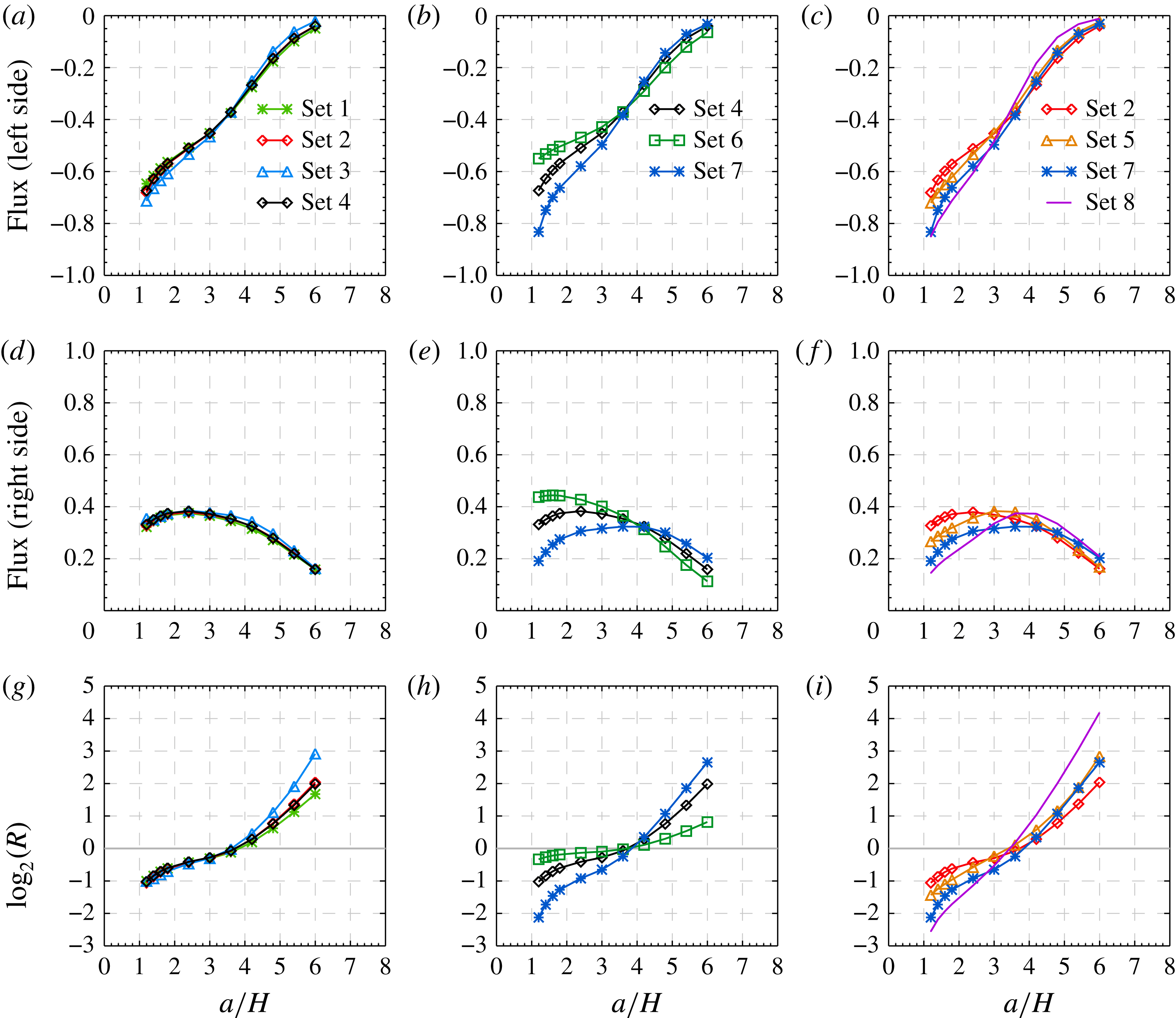
Figure 15. Tidally averaged energy fluxes at
 $t=20T$
scaled by
$t=20T$
scaled by
 $F_{0}$
as a function of the ridge width
$F_{0}$
as a function of the ridge width
 $a/H$
for eight sets of simulations. (a,d,g) Sets 1–4 (legend in panel a). In sets 1–3 the ridge amplitude is varied. Sets 2 and 4 have different shear layer thicknesses. (b,e,h) Sets 4, 6, 7 (legend in panel b) vary primarily in the strength of the current (
$a/H$
for eight sets of simulations. (a,d,g) Sets 1–4 (legend in panel a). In sets 1–3 the ridge amplitude is varied. Sets 2 and 4 have different shear layer thicknesses. (b,e,h) Sets 4, 6, 7 (legend in panel b) vary primarily in the strength of the current (
 $U_{s}/(NH)=0.1$
, 0.04 and 0.16 respectively). (c,f,i) Sets 2, 5, 7 and 8 (legend in panel c). Sets 2, 5 differ only in depth of the current as do sets 7 and 8. These two pairs of sets differ in the strength of the current. The first two rows show fluxes to the left and right of the ridge (at
$U_{s}/(NH)=0.1$
, 0.04 and 0.16 respectively). (c,f,i) Sets 2, 5, 7 and 8 (legend in panel c). Sets 2, 5 differ only in depth of the current as do sets 7 and 8. These two pairs of sets differ in the strength of the current. The first two rows show fluxes to the left and right of the ridge (at
 $\unicode[STIX]{x1D709}=3a/H$
and
$\unicode[STIX]{x1D709}=3a/H$
and
 $-3a/H$
). The third row shows the absolute value of the ratio of the rightward to leftward fluxes (log base 2).
$-3a/H$
). The third row shows the absolute value of the ratio of the rightward to leftward fluxes (log base 2).
Figure 16. Total tidally averaged energy fluxes
 $\langle E_{f}\rangle |_{\unicode[STIX]{x1D709}_{l}}^{\unicode[STIX]{x1D709}_{r}}$
radiating away from the ridge as a function of the ridge width. Values are at
$\langle E_{f}\rangle |_{\unicode[STIX]{x1D709}_{l}}^{\unicode[STIX]{x1D709}_{r}}$
radiating away from the ridge as a function of the ridge width. Values are at
 $t=20T$
and are scaled by
$t=20T$
and are scaled by
 $F_{0}$
.
$F_{0}$
.
 $\unicode[STIX]{x1D709}_{r}=3a/H$
and
$\unicode[STIX]{x1D709}_{r}=3a/H$
and
 $\unicode[STIX]{x1D709}_{l}=-3a/H$
.
$\unicode[STIX]{x1D709}_{l}=-3a/H$
.
The background current results in asymmetries in the upstream (leftward) and downstream (rightward) wave fields and energy fluxes. The results did not show strong sensitivity to the shear layer thickness; however, we only considered two similar values,
 $d_{s}/H=0.06$
and
$d_{s}/H=0.06$
and
 $0.08$
, to ensure the current was negligible at the crest of the ridge. Strengthening or deepening the current increased the asymmetries.
$0.08$
, to ensure the current was negligible at the crest of the ridge. Strengthening or deepening the current increased the asymmetries.
 $R$
, the ratio of the magnitude of the downstream and upstream energy fluxes, varied over a wide range of values. For each current this ratio increased monotonically as the ridge width increased, being considerably less than 1 for the narrowest ridge (
$R$
, the ratio of the magnitude of the downstream and upstream energy fluxes, varied over a wide range of values. For each current this ratio increased monotonically as the ridge width increased, being considerably less than 1 for the narrowest ridge (
 $a/H=1.2$
) and much larger than 1 for the widest ridge (
$a/H=1.2$
) and much larger than 1 for the widest ridge (
 $a/H=6$
), the transition point with
$a/H=6$
), the transition point with
 $R=1$
being approximately 3.5. For the widest ridge using a current of depth
$R=1$
being approximately 3.5. For the widest ridge using a current of depth
 $z_{s}/H=-0.3$
, the ratio increased from approximately 2 to 8 as the strength of the currents increased from
$z_{s}/H=-0.3$
, the ratio increased from approximately 2 to 8 as the strength of the currents increased from
 $U_{s}/NH=0.04$
to
$U_{s}/NH=0.04$
to
 $0.16$
while for the narrowest ridge
$0.16$
while for the narrowest ridge
 $R$
decreased from
$R$
decreased from
 $0.8$
to
$0.8$
to
 $0.25$
. Deepening the current increased these changes: for the strongest, deepest current (set 8)
$0.25$
. Deepening the current increased these changes: for the strongest, deepest current (set 8)
 $R=0.2$
for the narrowest ridge and 18 for the widest ridge.
$R=0.2$
for the narrowest ridge and 18 for the widest ridge.
In addition to introducing asymmetries in the energy fluxes in the upstream and downstream directions, the current has a significant effect on relative contributions of the various parts of the total flux. First, there is a leading-order contribution from the kinetic and available potential energy fluxes. The contribution from the available potential energy flux is small while that from the kinetic energy flux is significant. Furthermore, splitting the kinetic energy flux into contributions that are linear and quadratic in the velocity perturbation fields (from integrals of
 $\bar{U}^{2}u^{\prime }$
and
$\bar{U}^{2}u^{\prime }$
and
 $\bar{U}u^{\prime 2}$
respectively where
$\bar{U}u^{\prime 2}$
respectively where
 $u^{\prime }$
is the horizontal velocity perturbation) shows that the former is also significant for
$u^{\prime }$
is the horizontal velocity perturbation) shows that the former is also significant for
 $U_{s}/NH=0.1$
. This can only come from mean second-order fields. Similarly, splitting the mean work term into contributions that are linear and quadratic in the perturbation fields, i.e. from integrals of
$U_{s}/NH=0.1$
. This can only come from mean second-order fields. Similarly, splitting the mean work term into contributions that are linear and quadratic in the perturbation fields, i.e. from integrals of
 $\bar{U}p_{d}$
and
$\bar{U}p_{d}$
and
 $u^{\prime }p_{d}$
where
$u^{\prime }p_{d}$
where
 $p_{d}$
is the pressure perturbation, shows that the term linear in the pressure perturbation also makes a significant contribution. For the case with
$p_{d}$
is the pressure perturbation, shows that the term linear in the pressure perturbation also makes a significant contribution. For the case with
 $a/H=1.2$
and
$a/H=1.2$
and
 $U_{s}/NH=0.1$
shown in figure 12 the contribution from the terms linear in the perturbations is approximately 25 % of the total leftward energy flux.
$U_{s}/NH=0.1$
shown in figure 12 the contribution from the terms linear in the perturbations is approximately 25 % of the total leftward energy flux.
The tidally averaged mean fields show strong asymmetries about narrow ridges (figure 2) and are responsible for the tidally averaged work and kinetic energy flux terms undergoing significant quasi-periodic oscillations as a function of distance from the ridge. We leave further exploration of the mean currents to future work but note that the generation of mean currents when an internal wave beam impinges on a pycnocline has been observed in the laboratory (Mercier et al. Reference Mercier, Mathur, Gostiaux, Gerkema, Magalhães, Da Silva and Dauxois2012).
A linear theory, valid for small amplitude ridges and small tidal excursions, was developed to predict the leading-order perturbation fields. The fluxes based on the first-order solution (which does not include fluxes associated with second-order mean fields which are formally just as important) predicts spatially varying work and kinetic energy flux terms that agree well with the second-order fluxes from the nonlinear simulations for narrow ridges (see figure 12). These spatial variations arise because in the presence of a background current the linear eigenmodes are not orthogonal. Both the amplitude of the spatial oscillations and their wavelength seen in the nonlinear simulations is well predicted by the first-order linear theory. For the case illustrated in figure 12 the wavelength of the oscillations is equal to the distance between locations where beams reflect off the surface and is close to the wavelength associated with interactions of the mode-one and mode-two waves. For a much wider ridge (
 $a/H=6$
, figure 13) the agreement between first-order linear theory and the second-order perturbation fluxes is not as good but improves as the ridge amplitude decreases. This may be because as the ridge width increases waves above the ridge propagate for longer distances in slightly shallower water, an effect not taken into account by linear theory.
$a/H=6$
, figure 13) the agreement between first-order linear theory and the second-order perturbation fluxes is not as good but improves as the ridge amplitude decreases. This may be because as the ridge width increases waves above the ridge propagate for longer distances in slightly shallower water, an effect not taken into account by linear theory.
We have considered an idealized situation in a nearly linear regime. For more realistic stratifications with a strong subsurface pycnocline wave propagation speeds would be larger. For the same currents used here this would result in smaller Froude numbers presumably reducing the strength of the asymmetry in the upstream and downstream fluxes. This will be explored in future work. Other complicating factors include three-dimensional time varying background currents, multiple tidal constituents leading to spring-neap tidal cycles, three-dimensional bathymetry and horizontally varying stratifications. In addition rotational effects should be considered. It would be extremely difficult to separate any observed mean fields into a background state and wave-induced mean fields unless the wave-induced mean fields were much stronger than in our simulations as may potentially occur in shallower water with stronger tidal currents than those used here. Nevertheless the findings reported here suggest that in the presence of strong currents internal wave energy fluxes emanating away from a quasi-two-dimensional ridge can be strongly asymmetric with the direction of the largest energy fluxes being sensitive to the ridge width. The results also suggest that estimating the traditional work term
 $\int u^{\prime }p^{\prime }\,\text{d}z$
may not be sufficient: it may undergo significant spatial variations and contributions from the kinetic energy fluxes need to be considered. It should be possible to measure the latter and see if it is a significant fraction of the work term
$\int u^{\prime }p^{\prime }\,\text{d}z$
may not be sufficient: it may undergo significant spatial variations and contributions from the kinetic energy fluxes need to be considered. It should be possible to measure the latter and see if it is a significant fraction of the work term
 $\langle W\rangle$
which is traditionally measured.
$\langle W\rangle$
which is traditionally measured.
There are many possible avenues for future study. These include situations in which the bathymetry penetrates into the current as well as the effects of background currents on internal solitary wave generation when the stratification is non-constant, supercritical topography and three-dimensional effects. A full second-order theory which includes fluxes associated with second-order mean fields is desirable as is one not restricted to small amplitude topography. A possible avenue for the latter, which is restricted to small excursion distances, is a Green’s function approach similar to that developed for tide–topography interactions in the absence of a background current (Mathur, Carter & Peacock Reference Mathur, Carter and Peacock2016). The theory could also be extended to include a free surface.
In conclusion, the presence of a uni-directional surface trapped background current introduces asymmetries in the internal wave field and in the energy fluxes radiating upstream and downstream while the total energy flux away from the ridge is not significantly affected. This would likely not be the case if the ridge penetrated into the current. For narrow ridges the upstream fluxes can be 4–5 times larger than the downstream fluxes while for sufficiently wide ridges the downstream fluxes may be 8 or more times larger than the upstream fluxes. In addition the kinetic energy flux can be significant as can contributions from second-order mean fields.
Acknowledgements
This work is supported by grants from the Natural Sciences and Engineering Research Council of Canada and from the Canadian Foundation for Innovation and the Ontario Research Fund. The facilities of the Shared Hierarchical Academic Research Computing Network (SHARCNET: https://www.sharcnet.ca) and Compute/Calcul Canada were used for this work.


