


1. Introduction
Let $F = (f,\, g): {\mathbb {R}}^{2} \to {\mathbb {R}}^{2}$ be a polynomial map whose Jacobian determinant satisfies

for all $(x,\,y) \in {\mathbb {R}}^{2}$ . The map $F$
 is locally a diffeomorphism but, after the family of counterexamples found by Pinchuk [Reference Pinchuk15], we know that $F$
 is not necessarily globally injective. Pinchuk's counterexamples disprove the real Jacobian conjecture, i.e. the claim that polynomial maps satisfying (1) are injective.
A natural problem is then to look for additional conditions that guarantee the real Jacobian conjecture. For instance, if the Jacobian determinant of $F$ is a constant different from zero, then its injectivity is unknown up to now, and this problem is part of the famous Jacobian conjecture, which is unsolved until these days, see [Reference van den Essen9].
Conditions on the degree of $F$ were established in [Reference Braun and dos Santos Filho1,Reference Braun and Oréfice-Okamoto3,Reference Gwoździewicz13]. Conditions on the spectrum of $DF$
 , also valid for non-polynomial maps, can be found in [Reference Cobo, Gutierrez and Llibre7,Reference Fernandes, Gutierrez and Rabanal10]. The aim of this paper is to provide different conditions to the validity of the real Jacobian conjecture. Our main result is Theorem 1, which turns out to be a generalization of the main result of [Reference Braun, Giné and Llibre4]. Theorem 1 is also related to the work [Reference Cima, Gasull and Mañosas6], as explained below. In order to enunciate the theorem, we need some preliminary concepts.
Let $s_1$ and $s_2$
 be positive integers and set $s = (s_1,\,s_2)$
 . We say that a polynomial function $f \colon {\mathbb {R}}^{2} \to {\mathbb {R}}$
 is $s$
 -weight-homogeneous if there is a non-negative integer $d$
 such that
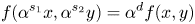
for all $\alpha \in {\mathbb {R}}$ , $\alpha > 0$
 , and for all $(x,\,y) \in {\mathbb {R}}^{2}$
 . In this case, we call $d$
 the weight-degree of $f$
 and $s$
 the weight-exponent of $f$
 . When $s = (1,\, 1)$
 we simply say that $f$
 is homogeneous of degree $d$
 . Given a weight-exponent $s$
 and a polynomial $f: {\mathbb {R}}^{2} \to {\mathbb {R}}$
 , we can uniquely write $f = f_0 + f_1 + \cdots + f_r$
 where $f_{i}$
 is a $s$
 -weight-homogeneous polynomial of weight degree $i$
 . In this case, when $f_r \neq 0$
 , we say that $f_r$
 is the higher $s$
 -weight-homogeneous part of $f$
 and we also say that $r$
 is the weight degree of $f$
 . It is straightforward to check the validity of the following Euler formula for a $s$
 -weight-homogeneous polynomial $f$
 with weight degree $d$
 :
:

Here $f_x$ (respectively $f_y$
 ) is the partial derivative of $f$
 with respect to $x$
 (respectively $y$
 ). It is also clear in this case that $f_x$
 (respectively $f_y$
 ) is $s$
 -weight-homogeneous with weight degree $d - s_1$
 (respectively $d - s_2$
 ). Finally, if $p(x,\,y) = (a x + b y)^{k} q(x,\,y)$
 , with $p$
 and $q$
 polynomial functions, $k$
 a positive integer and $a,\, b \in {\mathbb {R}}$
 , then we say that $a x + b y$
 is a real linear factor of $f$
 . We observe that a $s$
 -weight-homogeneous polynomial $p$
 , with $s_1 \neq s_2$
 , can have a real linear factor only in case $a = 0$
 or $b = 0$
 . Now we can formulate our main result.
Theorem 1 Let $F = (f,\,g) \colon {\mathbb {R}}^{2} \to {\mathbb {R}}^{2}$ be a polynomial map satisfying (1) and such that there is $z \in {\mathbb {R}}^{2}$
 with $F(z) = (0,\,0)$
 .
.
(a) If either the higher homogeneous terms of the polynomials $f f_x + g g_x$
 and $f f_y + g g_y$ do not have real linear factors in common, or
(b) if the higher homogeneous term of $f^{2} + g^{2}$
does not have a factor $(a x + b y)^{2},$ with $a b \neq 0,$ and there is a weight-exponent $s$ such that the higher $s$-weight-homogeneous terms of the polynomials $f f_x + g g_x$ and $f f_y + g g_y$ do not have real linear factors in common,


then $F$ is injective.
The main result of [Reference Braun, Giné and Llibre4] is only statement (a) of Theorem 1, with $z = (0,\,0)$ . The following is an example where the injectivity follows from Theorem 1 but not from [Reference Braun, Giné and Llibre4]. Let $F(x,\,y) = (x + y + x^{2},\, y + x^{2})$
 . We have $\det DF = 1$
 and
and

The higher homogeneous terms of these polynomials are $4 x^{3}$ and $2 x^{2}$
 , respectively, and so the assumptions of [Reference Braun, Giné and Llibre4] are not satisfied. Now the higher homogeneous term of $f^{2} + g^{2}$
 is $2 x^{4}$
 and, with weight exponent $s = (1,\, 2)$
 , the higher $s$
 -weight-homogeneous terms of the above polynomials are $4 x (y + x^{2})$
 and $2 (y + x^{2})$
 , respectively, that do not have real linear factors in common. So $F$
 is injective by Theorem 1.
We point out that the assumptions on Theorem 1 are not necessary for the global injectivity of a polynomial local diffeomorphism, as can be seen by the polynomial diffeomorphism $G(x,\,y) = (x+(x-y)^{2},\, y+(x-y)^{2})$ . Here $\det DG = 1$
 , the higher homogeneous part of $f^{2}+g^{2}$
 is $2 (x-y)^{4}$
 and the higher homogeneous terms of $f f_x+g g_x$
 and $f f_y + g g_y$
 are $4(x-y)^{3}$
 and $-4(x-y)^{3}$
 , respectively, and so we can not use Theorem 1.
It is important to mention here that a standard fact in algebraic geometry is that if a polynomial map $(f,\,g)$ satisfying (1) has no points at infinity in $\mathbb {RP}^{2}$
 , i.e., the higher homogeneous term of $f^{2}+g^{2}$
 has no real linear factors, then $(f,\,g)$
 is a proper map, and so it is a diffeomorphism, according to [Reference Randall16]. A generalization of this to the quasi-homogenous frame is the bidimensional counterpart of [Reference Cima, Gasull and Mañosas6, Theorem A]: polynomial maps $F = (f,\, g)$
 satisfying (1) and such that the higher $s$
 -weight-homogeneous parts of $f$
 and $g$
 have $(0,\,0)$
 as an isolated common zero, are injective. We observe that in the first example $F$
 above, the higher $s$
 -weight-homogenous parts of $f$
 and $g$
 are $(y,\, y)$
 , $(y + x^{2},\, y + x^{2})$
 or $(x^{2},\, x^{2})$
 , depending whether $2 s_1 < s_2$
 , $2 s_1 = s_2$
 or $2 s_1 > s_2$
 , respectively. None of them have $(0,\,0)$
 as an isolated common zero, and hence this example (satisfying the hypotheses of Theorem 1) does not satisfy the assumptions of [Reference Cima, Gasull and Mañosas6, Theorem A]. On the other hand, we do not know if our Theorem 1 implies this result of [Reference Cima, Gasull and Mañosas6], although in case the $s$
 -weight degree of $f$
 and $g$
 is equal, for some weight $s$
 , it does, as proven in Lemma 6.
We emphasize that our proofs rely on qualitative theory of differential equations and uses a characterization of injectivity of $F$ via centres of a suitable Hamiltonian vector field associated to $F$
 . In our reasoning, we prove a result on polynomial Hamiltonian vector fields in the plane, Proposition 4, which is a generalization of a result of [Reference Cima, Gasull and Mañosas5] that we think is interesting on its own.
In § 2, we summarize this and other results needed to the proof of Theorem 1, which is performed in § 3.
After the completion of this work, we took knowledge of the paper [Reference Mello and Xavier14], a partly expository paper with very nice connections between global injectivity and dynamics. The main result of [Reference Mello and Xavier14] is that a polynomial map $(f,\,g)$ satisfying (1) is globally injective provided the complexification of the algebraic curve $f=0$
 has one place at infinity (meaning that the curve $f=0$
 is irreducible and the pre-image of the desingularization map of the curve intersected with the infinity line in $\mathbb {CP}^{2}$
 has only one point, see the precise definition in [Reference Mello and Xavier14]). This result is different from our Theorem 1 as the polynomial local diffeomorphism $(f,\,g)(x,\,y) = (x+x^{3},\, y+y^{3} )$
 satisfies the assumption (a) of Theorem 1 but $f$
 and $g$
 are not irreducible, and so cannot have one place at infinity.
2. Preliminary results and a new condition for degenerate hyperbolic sectors at infinity
We begin this section by explaining the characterization of injectivity of polynomial maps mentioned in the introduction section. By a centre of a vector field $\mathcal {V}$ , we mean as usually an equilibrium point $v$
 of $\mathcal {V}$
 having a neighbourhood $U$
 such that $U \setminus \{v\}$
 is filled with non-constant periodic orbits of $\mathcal {V}$
 . The period annulus of the centre is the maximum neighbourhood of $v$
 with this property. We say that a centre is global if its period annulus is the whole plane.
In what follows we assume that $F = (f,\, g)$ is a polynomial map satisfying (1). Let the function $H \colon {\mathbb {R}}^{2} \to {\mathbb {R}}$
 be defined by
for $(x,\,y) \in {\mathbb {R}}^{2}$ and its associated Hamiltonian vector field $\chi = (P,\,Q)$
 , that is,

We observe that $q \in {\mathbb {R}}^{2}$ is a singular point of $\chi$
 if and only if $DF(q)\cdot q = (0,\,0)$
 , which is equivalent to $F(q) = (0,\,0)$
 as $\det DF(q) \ne 0$
 . Let $U$
 be a neighbourhood of $q$
 where $F$
 is injective. It follows that $H$
 is positive in all the points of $U$
 different from $q$
 , while $H(q) = 0$
 , proving that $q$
 is an isolated minimum of $H$
 . Then all the orbits of $\chi$
 in a neighbourhood of $q$
 (maybe smaller than $U$
 ) are closed, proving that $q$
 is a centre of $X$
 . We state this result as a lemma for further reference.
Lemma 2 The singular points of $\chi$ are the zeros of $F$
 . Each of them corresponds to a centre of $\chi,$
 and so has index $1$
 .
.
The following is a generalization given in [Reference Braun and Llibre2] of a result from [Reference Sabatini17], see also [Reference Gavrilov11]:
Theorem 3 Let $F: {\mathbb {R}}^{2} \to {\mathbb {R}}^{2}$ be a polynomial map satisfying (1). Assume there is $z \in {\mathbb {R}}^{2}$
 such that $F(z) = (0,\,0)$
 . Then $F$
 is injective if and only if the centre $z$
 of $\chi$
 is global.
In what follows we use results and notation on the Poincaré compactification of polynomial vector fields of $ {\mathbb {R}}^{2}$ . Particularly, $U_i$
 , $V_i$
 , $i=1,\,2,\,3$
 , are the canonical local charts of the Poincaré sphere $\mathbb {S}^{2}$
 . For details on this technique, we refer the reader to [Reference Dumortier, Llibre and Artés8, Chapter 5] or to [Reference González-Velasco12]. Letting $X$
 be a polynomial vector field of $ {\mathbb {R}}^{2}$
 , we denote by $p(X)$
 its compactification. As usual, we say that $q$
 is an infinite singular point of $X$
 , or of $p(X)$
 , if $q$
 is in the equator of $\mathbb {S}^{2}$
 . We also say that a hyperbolic sector $h$
 of $q$
 is degenerate if its two separatrices are contained in the equator of $\mathbb {S}^{2}$
 . Finally, by the Poincaré disc, we mean the projection of the north hemisphere together with the equator of $\mathbb {S}^{2}$
 on the plane $z = 0$
 .
.
Next result studies the infinite singular points of a general polynomial Hamiltonian vector field, giving necessary conditions in order to have a non-degenerate hyperbolic sector. It turns out that the present result generalizes a similar result from [Reference Cima, Gasull and Mañosas5], by considering also weight-homogeneous polynomials. We recall that for a Hamiltonian vector field $X = (-H_y,\, H_x)$ , where $H: {\mathbb {R}}^{2} \to {\mathbb {R}}$
 is a polynomial, the infinite singular points of $p(X)$
 in the Poincaré disc are the endpoints of each straight line $a x + b y = 0$
 , where $a x + b y$
 is a real linear factor of the higher homogeneous part of $H$
 .
.
Proposition 4 Let $q$ be an infinite singular point of a Hamiltonian system $X = (P,\,Q) = (-H_y,\,H_x)$
 (with $PQ \not \equiv 0$
 ), endpoint of the straight line $a x + b y = 0$
 in the Poincaré disc. If $q$
 has a non-degenerate hyperbolic sector, then $ax + by$
 is a common factor of the higher homogeneous parts of $P$
 and $Q$
 . If $a = 0$
 (respectively $b = 0$
 ), then $y$
 (respectively $x$
 ) is a common factor of the higher $s$
 -weight-homogeneous parts of $P$
 and $Q,$
 for each weight-exponent $s = (s_1,\, s_2)$
 .
.
Proof. We clearly can assume that the degree of $H$ is greater than $1$
 and that the higher homogeneous term of $H$
 has the form

where $\tau \geq 1$ is an integer and $r(x,\,y)$
 is a polynomial that does not have $a x + b y$
 as a factor.
Clearly if $a b \neq 0$ and $\tau \geq 2$
 , then the higher homogeneous terms of $P$
 and $Q$
 have both the factor $a x + b y$
 , and we are done.
So it remains to consider the following three cases concerning the higher homogeneous term of $H$ : (i) it has the form $r(x,\,y)(a x + b y)$
 with $a b \neq 0$
 , i.e., $\tau = 1$
 ; or (ii) it has the form $r(x,\,y) y^{\tau }$
 , i.e., $a = 0$
 ; or (iii) it has the form $r(x,\,y) x^{\tau }$
 , i.e., $b = 0$
 . By changing $x$
 and $y$
 we do not need to consider case (iii) (observe that with a change like that, a $(s_1,\, s_2)$
 -weight-homogeneous polynomial is carried to a $(s_2,\, s_1)$
 -weight-homogeneous polynomial). Also, with a linear change of variable we can transform (i) into (ii) and consider just the later case (because the degree of $H$
 is greater than $1$
 ). Our conclusion will show that case (ii) with $\tau = 1$
 (and so case (i)) cannot happen.
So we assume that case (ii) is in force. Letting $s = (s_1,\, s_2)$ be a given weight-exponent, we denote by $m$
 and $n$
 the weight degrees with respect to $s$
 of $P$
 and $Q$
 , respectively. In the sequel, we shall use notation on the Poincaré compactification of $X$
 . Observe that $q$
 is the origin of the local chart $U_1$
 , that we will treat with the variables $(u,\,v)$
 , with the relation between $(x,\,y)$
 and $(u,\,v)$
 given by $(u,\,v) = (y/x,\,1/x)$
 . The equator of the Poincaré sphere, i.e., the infinite of $ {\mathbb {R}}^{2}$
 is mapped in the straight line $v = 0$
 . Let $r_1$
 and $r_2$
 be the two separatrices of a hyperbolic sector $h$
 of $(0,\,0)$
 in $U_1$
 . Without loss of generality, we assume that the interior of $h$
 is contained in the region $v > 0$
 . Suppose that $r_1$
 is not contained in the infinite, i.e. in the straight line $v = 0$
 . We claim that $r_2$
 is not contained in the infinite and that $r_1$
 and $r_2$
 have the same tangent line at $(0,\,0)$
 . Indeed, assume on the contrary that there exists a straight half-line $u = \lambda v$
 , with $v > 0$
 , between $r_1$
 and $r_2$
 . Each obit of $X$
 is contained in a level set of $H(x,\,y) = c$
 of $H$
 . So, by letting

and $\tilde G(u,\,v) = \tilde H(u,\,v)/v^{d+1}$ , points $(u,\,v)$
 of the compactified orbit will satisfy $\tilde G(u,\,v) = c$
 . Let $c$
 be the value of $\tilde G$
 in $r_1$
 . Since $h$
 is an hyperbolic sector, each sequence $\{w_n\}$
 in the interior of $h$
 such that $\lim _{n \to \infty } w_n = (0,\,0)$
 will satisfy $\lim _{n \to \infty }\tilde G(w_n) = c$
 . So
. So

Then writing $\tilde H = \sum \nolimits _{i = 0}^{d+1} \tilde H_i$ , with $\tilde H_i$
 being the homogeneous part of degree $i$
 of $\tilde H$
 , we get $\tilde H_0(\lambda,\,1) = \cdots = \tilde H_d(\lambda,\, 1) = 0$
 and $\tilde H_{d+1}(\lambda,\, 1) = c$
 . Hence

meaning that the straight half-line $u = \lambda v$ is invariant by the flow, a contradiction. This proves the claim.
Clearly $\tilde G(u,\,v)$ have the same value $c$
 in $r_1$
 and $r_2$
 , by the continuity of $\tilde G$
 in $v > 0$
 . Let $u = \lambda v$
 , $v > 0$
 , the common tangent of $r_1$
 and $r_2$
 at $(0,\,0)$
 . This line is contained in the tangent cone of the algebraic variety $\tilde H(u,\,v) - c v^{d+1} = 0$
 , with multiplicity at least two, i.e.,

with $k \geq 2$ and $\tilde {\tilde H}_{k}(u,\,v) = (u - \lambda v)^{2} R(u,\,v)$
 , where $R(u,\,v)$
 is a homogeneous polynomial of degree $k - 2$
 , and $\tilde { \tilde H}_i$
 is the homogeneous part of degree $i$
 of $\tilde H(u,\,v) - c v^{d+1}$
 . Therefore, from (3), it follows that

Note that if $k = d+1$ then $H(x,\,y) = \tilde H_{d+1}(y)$
 which is not possible because then $Q \equiv 0$
 . So, $k < d+1$
 , and $Q$
 contains the term $(d + 1 - k) x^{d-k} \tilde {\tilde H}_k(y,\,1)$
 . Since $\tilde H_k=(y-\lambda )^{2} \tilde R(y,\,1)$
 we get that $n$
 , which is the $s$
 -weight degree of $Q$
 , satisfies
The $s$ -weight-homogeneous part of weight degree $n$
 of $Q$
 writes

Since the maximum exponent of $x$ in $H$
 is $d + 1 - k$
 , and so the maximum possible exponent of $x$
 in $Q_n$
 is $d - k$
 , it follows that if $a_{i j} \neq 0$
 in the above sum, then $(d-k) s_1 + j s_2 \geq n \geq (d-k) s_1 + 2 s_2$
 , from (4), forcing that $j$
 is at least $2$
 . This means that

where $T(x,\,y)$ is a suitable $s$
 -weight-homogeneous polynomial of weight degree $n - 2 s_2$
 . Since $Q_n = \partial H_{n + s_1}/\partial x$
 , where here $H_{n+s_1}$
 means the $s$
 -weight-homogeneous term of weight degree $n + s_1$
 of $H$
 (recall that if $H$
 has $s$
 -weight degree $\ell$
 then $\partial H/\partial x$
 , if not zero, has $s$
 -weight degree $\ell - s_1$
 ), it thus follows that

for some polynomial $G(y)$ which must be a factor of $y^{2}$
 , otherwise $H_{n + s_1}$
 is not weight-homogeneous.
Now the higher $s$ -weight-homogeneous term, $P_m$
 , of $P = -H_y$
 comes from $H_{m + s_ 2}$
 . Clearly $m + s_2 \geq n + s_1$
 by (5). In case $m + s_2 = n + s_1$
 , then $P_m$
 has a factor $y$
 . On the other hand, if $m + s_2 > n + s_1$
 , it follows that $H_{m + s_2} = s y^{j}$
 , with $s_2 j = m + s_2$
 , otherwise the higher $s$
 -weight-homogeneous term of $Q$
 is not $Q_n$
 because $m + s_2 - s_1 > n$
 . In particular, $P_m$
 has a factor $y$
 .
.
Observe that our proof shows in particular that the higher $s$ -weight-homogeneous term of $H$
 has the factor $(a x + b y)^{2}$
 (homogeneous if $a b \neq 0$
 ). In particular, case (i) of the beginning of the proof is not possible.
Corollary 5 Let $H \colon {\mathbb {R}}^{2} \to {\mathbb {R}}$ be a polynomial function. Let $q$
 be an infinite singular point of the polynomial Hamiltonian vector field $\chi = (-H_y,\,H_x)$
 , endpoint of the straight line $a x + b y = 0$
 in the Poincaré disc. Assume either that the higher homogeneous terms of $H_x$
 and $H_y$
 do not have real linear factors in common, or, if $a = 0,$
 (respectively $b = 0$
 ) that $y$
 (respectively $x$
 ) is not a common factor of the higher $s$
 -weight-homogeneous parts of $H_x$
 and $H_y,$
 for some weight-exponent $s = (s_1,\, s_2)$
 . Then the topological index of $q$
 is greater than or equal to zero. If this index is zero, then $q$
 is formed by two degenerate hyperbolic sectors.
Proof. From Proposition 4, it follows that $q$ have no non-degenerate hyperbolic sectors. Thus, the number of hyperbolic sectors of $q$
 is $h \leq 2$
 . By the index formula we conclude that the index of $q$
 is greater than or equal to the number of elliptic sectors of $q$
 , and so greater than or equal to zero. If the index is zero, it thus clearly follows that there are no elliptic sectors and also that $q$
 must have two degenerate hyperbolic sectors.
3. Proof of Theorem 1
We consider the function $H(x,\,y) = (f(x,\,y)^{2} + g(x,\,y)^{2})/2$ defined in $ {\mathbb {R}}^{2}$
 , and the associated Hamiltonian vector field $\chi = (- H_y,\, H_x )$
 . Since $F(z) = (0,\,0)$
 , it follows from Theorem 3 that in order to prove that $F$
 is injective, it is enough to prove that $z$
 is a global centre of the vector field $\chi$
 .
.
Let $q$ be an infinite singular point of $\chi$
 , endpoint of the straight line $a x + b y = 0$
 in the Poincaré disc. If we are under assumption (a) of Theorem 1, then we are under the assumptions of Corollary 5. If we assume (b) of the Theorem and $a b \neq 0$
 , then $a x + b y$
 is not a common factor of $H_x$
 and $H_y$
 (from (2)), and we are again under the assumptions of Corollary 5. On the other hand, if $a b = 0$
 , assumption (b) guarantees the existence of a weight-exponent $s$
 satisfying the assumptions of Corollary 5. Thus, in any case, it follows from this corollary that the topological index of any infinite singular point of $\chi$
 is greater than or equal to zero.
Also, the index of each finite singular point of $\chi$ is one, by Lemma 2. Corresponding to the singular point $z$
 of $\chi$
 there are two singular points of $p(\chi )$
 , the Poincaré compactification of $\chi$
 , one in each hemisphere of the Poincaré sphere, having index $1$
 . Thus the sum of the indices of all the singular points of $p(\chi )$
 in the Poincaré sphere is at least $2$
 . From the Poincaré–Hopf theorem (see Theorem 6.30 in[Reference Dumortier, Llibre and Artés8]), this sum must be $2$
 . So, we conclude that $p(\chi )$
 does not have other finite singular points (other than the two centres corresponding to the centre of $\chi$
 ) and $p(\chi )$
 either does not have infinite singular points or each of them has index $0$
 , which again by Corollary 5, must be formed by two degenerate hyperbolic sectors.
Looking at the Poincaré disc, we summarize the frame: $\chi$ is a polynomial vector field such that its Poincaré compactification $p(\chi )$
 in the Poincaré disc has a centre in its only finite singular point, and $p(\chi )$
 either does not have infinite singular points or they are formed by degenerate hyperbolic sectors. From this, it is not difficult to conclude that $z$
 must be a global centre of $\chi$
 (see, for instance, Corollary 10 and the proof of Theorem 1 in [Reference Braun, Giné and Llibre4]).
We end the paper with the following Lemma, that gives a relation between our Theorem and the already mentioned result of [Reference Cima, Gasull and Mañosas6].
Lemma 6 Let $F = (f,\,g) \colon {\mathbb {R}}^{2} \to {\mathbb {R}}^{2}$ be a polynomial map and let $s = (s_1,\, s_2)$
 be a weight-exponent. Assume that the weight degrees of $f$
 and $g$
 with respect to $s$
 are equal. If the higher $s$
 -weight-homogeneous terms of $f$
 and $g$
 do not have real linear factors in common, then so do the higher $s$
 -weight-homogeneous terms of $f f_x + g g_x$
 and $f f_y + gg_y$
 .
.
Proof. We let $m$ be the weight degree of $f$
 and $g$
 and write $f = f_0 + \cdots + f_m$
 and $g = g_0 + \cdots + g_m$
 the weight decomposition of $f$
 and $g$
 . We first observe that $(f_m^{2} + g_m^{2})_x \not \equiv 0$
 and $(f_m^{2} + g_m^{2})_y \not \equiv 0$
 , because if $(f_m^{2} +g_m^{2})_x \equiv 0$
 , for instance, then (we are dealing with polynomials) $f_m = a_{0\ell } y^{\ell }$
 and $g_m = b_{0\ell } y^{\ell }$
 , with $\ell s_2 = m$
 and $a_{0\ell },\, b_{0\ell } \in {\mathbb {R}}$
 , a contradiction.
Thus, the higher $s$ -weigh-homogeneous parts of $f f_x + g g_x$
 and $f f_y + g g_y$
 are, respectively, $(f_m^{2} + g_m^{2})_x/2$
 and $(f_m^{2} + g_m^{2})_y/2$
 . If there is a linear factor dividing the last polynomials, it will also divide

and so this factor will be common to $f_m$ and $g_m$
 , a contradiction.
This lemma is no longer true without the assumption that the weight degrees of $f$ and $g$
 are the same, as the map $F(x,\,y) = (x+y^{3},\,y-x^{3})$
 shows. It satisfies $\det DF = 1+9 x^{2} y^{2}$
 and, with $s=(3,\,1)$
 , the higher homogeneous terms of $f$
 and $g$
 are $x+y^{3}$
 and $=x^{3}$
 , respectively. But the higher homogeneous terms of $f f_x + g g_x$
 and $f f_y + g g_y$
 are $3 x^{5}$
 and $-x^{3}$
 , respectively. Here it is worth to mention that with $s = (5,\,3)$
 , the higher $s$
 -weight-homogeneous terms of $f f_x +g g_x$
 and $f f_y + g g_y$
 are $3 x^{5}$
 and $-x^{3}+3 y^{5}$
 , respectively. That is, this map satisfies the assumption of Theorem 1.
Acknowledgements
The first named author was partially supported by the grant $2017$ /$00136$
 -$0$
-$0$ , São Paulo Research Foundation (FAPESP). The second named author was partially supported by FCT/Portugal through UID/MAT/$04459$
 /$2013$
 .
.


