


1 Introduction
Internal solitary waves are ubiquitous features in the coastal ocean, often having large amplitudes and strong currents. One of the strongest internal solitary waves on record has an amplitude of 240 m, and a peak current velocity of
 $2.55~\text{m}~\text{s}^{-1}$
, captured at a mooring site deployed in the northern South China Sea at the bottom depth of 3847 m, see Huang et al. (Reference Huang, Chen, Zhao, Zhang, Zhou, Yang and Tian2016). These waves are important as their energy and mass transport can produce a substantial impact on coastal marine engineering, marine biology and geology. Although mode-1 waves are those most commonly found in the ocean, there have been several recent observations and numerical simulations suggesting that mode-2 waves can also be present in some circumstances, see Farmer & Smith (Reference Farmer and Smith1980), Konyaev, Sabinin & Serebryany (Reference Konyaev, Sabinin and Serebryany1995), Stastna & Peltier (Reference Stastna and Peltier2005), Moum, Nash & Klymak (Reference Moum, Nash and Klymak2008), Yang et al. (Reference Yang, Fang, Chang, Ramp, Kao and Tang2009), Shroyer, Moum & Nash (Reference Shroyer, Moum and Nash2010), Yang et al. (Reference Yang, Fang, Tang and Ramp2010), Liu et al. (Reference Liu, Su, Hsu, Kuo and Ho2013). Mode-2 internal waves are usually not as energetic as mode-1 waves, but they can be significant for mixing shelf waters, especially as their location is usually in the middle of the pycnocline, and hence they can be effective in eroding the barrier between the upper mixed layer and the deep water below. Mode-2 internal solitary waves first came to notice in the laboratory experiments of Davis & Acrivos (Reference Davis and Acrivos1967) who examined the propagation of internal solitary waves in thin pycnocline embedded between two deep fluid layers. Like their mode-1 counterparts, mode-2 waves can be classified as elevation or depression, related theoretically to whether the nonlinear coefficient in the underlying Korteweg-de Vries equation is positive or negative. For mode-2 waves, an elevation wave is often called a ‘convex wave’ as the upper (lower) pycnocline interface is displaced upwards (downwards). In contrast a mode-2 depression wave is a ‘concave’ wave, with an hourglass-shaped structure, as the upper (lower) pycnocline interface is displaced downwards (upwards).
$2.55~\text{m}~\text{s}^{-1}$
, captured at a mooring site deployed in the northern South China Sea at the bottom depth of 3847 m, see Huang et al. (Reference Huang, Chen, Zhao, Zhang, Zhou, Yang and Tian2016). These waves are important as their energy and mass transport can produce a substantial impact on coastal marine engineering, marine biology and geology. Although mode-1 waves are those most commonly found in the ocean, there have been several recent observations and numerical simulations suggesting that mode-2 waves can also be present in some circumstances, see Farmer & Smith (Reference Farmer and Smith1980), Konyaev, Sabinin & Serebryany (Reference Konyaev, Sabinin and Serebryany1995), Stastna & Peltier (Reference Stastna and Peltier2005), Moum, Nash & Klymak (Reference Moum, Nash and Klymak2008), Yang et al. (Reference Yang, Fang, Chang, Ramp, Kao and Tang2009), Shroyer, Moum & Nash (Reference Shroyer, Moum and Nash2010), Yang et al. (Reference Yang, Fang, Tang and Ramp2010), Liu et al. (Reference Liu, Su, Hsu, Kuo and Ho2013). Mode-2 internal waves are usually not as energetic as mode-1 waves, but they can be significant for mixing shelf waters, especially as their location is usually in the middle of the pycnocline, and hence they can be effective in eroding the barrier between the upper mixed layer and the deep water below. Mode-2 internal solitary waves first came to notice in the laboratory experiments of Davis & Acrivos (Reference Davis and Acrivos1967) who examined the propagation of internal solitary waves in thin pycnocline embedded between two deep fluid layers. Like their mode-1 counterparts, mode-2 waves can be classified as elevation or depression, related theoretically to whether the nonlinear coefficient in the underlying Korteweg-de Vries equation is positive or negative. For mode-2 waves, an elevation wave is often called a ‘convex wave’ as the upper (lower) pycnocline interface is displaced upwards (downwards). In contrast a mode-2 depression wave is a ‘concave’ wave, with an hourglass-shaped structure, as the upper (lower) pycnocline interface is displaced downwards (upwards).
The deformation and possible disintegration of an oceanic internal solitary wave as it propagates over topography, typically from deep to shallow water, has been heavily studied and is now well understood, see the reviews by Grimshaw (Reference Grimshaw2006), Grimshaw, Pelinovsky & Talipova (Reference Grimshaw, Pelinovsky and Talipova2007), Grimshaw et al. (Reference Grimshaw, Pelinovsky, Talipova and Kurkina2010). However, nearly all previous work has been for mode-1 internal solitary waves, and there is an insufficient understanding of the shoaling process of the mode-2 waves, although we note the recent numerical studies by Guo & Chen (Reference Guo and Chen2012) of a mode-2 internal solitary wave shoaling on a slope in a model configuration close to the situation in the South China Sea, and by Terletska et al. (Reference Terletska, Jung, Talipova, Maderich, Brovchenko and Grimshaw2016) of the impact of a mode-2 internal solitary wave onto a vertical step in a three-layer fluid configuration. We also note the numerical simulations of Stastna & Peltier (Reference Stastna and Peltier2005) who showed that mode-2 waves could be generated in some circumstances by trans-critical flow over topography. Hence in this paper we examine the analogous problem for a mode-2 internal solitary wave propagating from deep to shallow water up the continental slope, where the water depth
 $h$
is slowly varying, in contrast to the abrupt step considered in Terletska et al. (Reference Terletska, Jung, Talipova, Maderich, Brovchenko and Grimshaw2016).
$h$
is slowly varying, in contrast to the abrupt step considered in Terletska et al. (Reference Terletska, Jung, Talipova, Maderich, Brovchenko and Grimshaw2016).
We use two complementary methodologies, both with a two-dimensional three-layer fluid model, which can support mode-2 waves. Initially a variable-coefficient Korteweg-de Vries (vKdV) equation is implemented to simulate the propagation of a mode-2 internal solitary wave from a flat deep ocean onto a slope, leading to a flat shallow ocean. Such vKdV equations have been commonly used to model mode-1 waves, and the structure of the equation is of course the same for mode-2 waves. Crucially the coefficients in the mode-2 case depend in a quite different way on the fluid depth than in the mode-1 case. Nevertheless, in the vKdV context the behaviour of an internal solitary wave in this mode-2 case can be inferred from the known results from the analogous mode-1 case, see Grimshaw (Reference Grimshaw2006), Grimshaw et al. (Reference Grimshaw, Pelinovsky and Talipova2007, Reference Grimshaw, Pelinovsky, Talipova and Kurkina2010). Suppose that, as the waves propagate from deep to shallow water up the continental slope, there is no polarity change, that is the nonlinear coefficient
 $\unicode[STIX]{x1D6FC}$
does not change sign over the slope. Then due to the conservation of wave-action flux, an adiabatic law
$\unicode[STIX]{x1D6FC}$
does not change sign over the slope. Then due to the conservation of wave-action flux, an adiabatic law
 $a^{3}\propto \unicode[STIX]{x1D6FC}$
relates the solitary wave amplitude
$a^{3}\propto \unicode[STIX]{x1D6FC}$
relates the solitary wave amplitude
 $a$
with the coefficient
$a$
with the coefficient
 $\unicode[STIX]{x1D6FC}$
. At the same time, to conserve mass, the deforming solitary wave is accompanied by a trailing shelf. But if there is a polarity change on the slope, which means
$\unicode[STIX]{x1D6FC}$
. At the same time, to conserve mass, the deforming solitary wave is accompanied by a trailing shelf. But if there is a polarity change on the slope, which means
 $\unicode[STIX]{x1D6FC}$
reaches zero at a certain critical point on the slope, then the adiabatic law breaks down as the wave approaches this critical point. After that the whole wave system transits this critical point, and the original incident wave develops into a leading rarefaction wave of the same polarity, on which rides a solitary wave train of the opposite polarity. As the vKdV equation is based on the weakly nonlinear long-wave regime, a complementary fully nonlinear non-hydrostatic MIT general circulation model (MITgcm) is also used here. Importantly, unlike the vKdV model, these simulations are not restricted to a single vertical mode, and can detect the possible generation of mode-1 waves during the propagation up the slope, as found by Terletska et al. (Reference Terletska, Jung, Talipova, Maderich, Brovchenko and Grimshaw2016) when a mode-2 wave impacts a vertical step. In particular the MITgcm model can be used to study the case when the three-layer stratification terminates on the slope and thereafter there is only a two-layer stratification. In this scenario, the mode-2 cannot exist on the shelf anymore, and any wave disturbance reaching the shelf must be a mode-1 wave.
$\unicode[STIX]{x1D6FC}$
reaches zero at a certain critical point on the slope, then the adiabatic law breaks down as the wave approaches this critical point. After that the whole wave system transits this critical point, and the original incident wave develops into a leading rarefaction wave of the same polarity, on which rides a solitary wave train of the opposite polarity. As the vKdV equation is based on the weakly nonlinear long-wave regime, a complementary fully nonlinear non-hydrostatic MIT general circulation model (MITgcm) is also used here. Importantly, unlike the vKdV model, these simulations are not restricted to a single vertical mode, and can detect the possible generation of mode-1 waves during the propagation up the slope, as found by Terletska et al. (Reference Terletska, Jung, Talipova, Maderich, Brovchenko and Grimshaw2016) when a mode-2 wave impacts a vertical step. In particular the MITgcm model can be used to study the case when the three-layer stratification terminates on the slope and thereafter there is only a two-layer stratification. In this scenario, the mode-2 cannot exist on the shelf anymore, and any wave disturbance reaching the shelf must be a mode-1 wave.
This paper is organised as follows. In § 2, we present the vKdV theory and a mode decomposition technique, used to analyse the output from the MITgcm, together with an analysis of the energy budget. Then in § 3 we discuss a three-layer configuration and derive the coefficients of the vKdV equation. Next the result of the shoaling process from a three-layer to a three-layer system, and from a three-layer to a two-layer system are presented in §§ 4 and 5 respectively. We conclude in § 6.
2 Formulation
The vKdV equation commonly used to describe internal waves in the coastal ocean, in the usual physical variables (see the reviews by Grimshaw (Reference Grimshaw2006), Grimshaw et al. (Reference Grimshaw, Pelinovsky and Talipova2007, Reference Grimshaw, Pelinovsky, Talipova and Kurkina2010) and the references therein) is
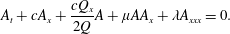 $$\begin{eqnarray}A_{t}+cA_{x}+\frac{cQ_{x}}{2Q}A+\unicode[STIX]{x1D707}AA_{x}+\unicode[STIX]{x1D706}A_{xxx}=0.\end{eqnarray}$$
Here
 $A(x,t)$
is the amplitude of the wave,
$A(x,t)$
is the amplitude of the wave,
 $x,t$
are space and time variables and subscripts denote derivatives. The coefficient
$x,t$
are space and time variables and subscripts denote derivatives. The coefficient
 $c$
is the relevant linear long-wave speed, and
$c$
is the relevant linear long-wave speed, and
 $Q$
is the linear magnification factor, explicitly defined below in (2.14) so that
$Q$
is the linear magnification factor, explicitly defined below in (2.14) so that
 $QA^{2}$
is the linear long-wave wave-action flux. The coefficients
$QA^{2}$
is the linear long-wave wave-action flux. The coefficients
 $\unicode[STIX]{x1D707}$
and
$\unicode[STIX]{x1D707}$
and
 $\unicode[STIX]{x1D706}$
of the nonlinear and dispersive terms are determined by the waveguide properties of the specific physical system, and for the present oceanic application, are defined below. For a variable medium, each of these is a slowly varying function of
$\unicode[STIX]{x1D706}$
of the nonlinear and dispersive terms are determined by the waveguide properties of the specific physical system, and for the present oceanic application, are defined below. For a variable medium, each of these is a slowly varying function of
 $x$
. The derivation of the vKdV equation (2.1) assumes the usual KdV balance that the nonlinear term
$x$
. The derivation of the vKdV equation (2.1) assumes the usual KdV balance that the nonlinear term
 $AA_{x}$
has the same order as the linear dispersive term
$AA_{x}$
has the same order as the linear dispersive term
 $A_{xxx}$
, so that formally the amplitude
$A_{xxx}$
, so that formally the amplitude
 $A$
is of the same order as
$A$
is of the same order as
 $\unicode[STIX]{x2202}^{2}/\unicode[STIX]{x2202}x^{2}$
. In addition the derivation assumes that the waveguide properties (that is, the coefficients
$\unicode[STIX]{x2202}^{2}/\unicode[STIX]{x2202}x^{2}$
. In addition the derivation assumes that the waveguide properties (that is, the coefficients
 $c,Q,\unicode[STIX]{x1D707},\unicode[STIX]{x1D706}$
) vary slowly so that
$c,Q,\unicode[STIX]{x1D707},\unicode[STIX]{x1D706}$
) vary slowly so that
 $Q_{x}/Q$
for instance is of the same order as the linear dispersive term. In this scenario, the first two terms in (2.1) are the dominant terms, and it is convenient and useful to make a transformation
$Q_{x}/Q$
for instance is of the same order as the linear dispersive term. In this scenario, the first two terms in (2.1) are the dominant terms, and it is convenient and useful to make a transformation
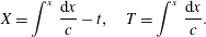 $$\begin{eqnarray}X=\int ^{x}\,\frac{\text{d}x}{c}-t,\quad T=\int ^{x}\,\frac{\text{d}x}{c}.\end{eqnarray}$$
Then, to the same order of asymptotic approximation as in the derivation of (2.1),
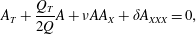 $$\begin{eqnarray}A_{T}+\frac{Q_{T}}{2Q}A+\unicode[STIX]{x1D708}AA_{X}+\unicode[STIX]{x1D6FF}A_{XXX}=0,\end{eqnarray}$$
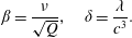
 $$\begin{eqnarray}\unicode[STIX]{x1D708}=\frac{\unicode[STIX]{x1D707}}{c},\quad \unicode[STIX]{x1D6FF}=\frac{\unicode[STIX]{x1D706}}{c^{3}}.\end{eqnarray}$$
A further simplification is
 $$\begin{eqnarray}U=A\sqrt{Q},\quad U_{T}+\unicode[STIX]{x1D6FD}UU_{X}+\unicode[STIX]{x1D6FF}U_{XXX}=0,\end{eqnarray}$$
 $$\begin{eqnarray}\unicode[STIX]{x1D6FD}=\frac{\unicode[STIX]{x1D708}}{\sqrt{Q}},\quad \unicode[STIX]{x1D6FF}=\frac{\unicode[STIX]{x1D706}}{c^{3}}.\end{eqnarray}$$
Here the coefficients
 $\unicode[STIX]{x1D6FD},\unicode[STIX]{x1D6FF}$
are functions of
$\unicode[STIX]{x1D6FD},\unicode[STIX]{x1D6FF}$
are functions of
 $T$
alone. Note that although
$T$
alone. Note that although
 $T$
is a variable along the spatial path of the wave, we shall subsequently refer to it as the ‘time’. Similarly, although
$T$
is a variable along the spatial path of the wave, we shall subsequently refer to it as the ‘time’. Similarly, although
 $X$
is a temporal variable, in a reference frame moving with speed
$X$
is a temporal variable, in a reference frame moving with speed
 $c$
, we shall subsequently refer to it as a ‘space’ variable. To simplify the calculation, a final transformation yields the canonical form,
$c$
, we shall subsequently refer to it as a ‘space’ variable. To simplify the calculation, a final transformation yields the canonical form,
 $$\begin{eqnarray}U_{\unicode[STIX]{x1D70F}}+\unicode[STIX]{x1D6FC}UU_{X}+U_{XXX}=0,\end{eqnarray}$$
 $$\begin{eqnarray}\text{where}~\unicode[STIX]{x1D70F}=\int ^{T}\unicode[STIX]{x1D6FF}\,\text{d}T,\quad \unicode[STIX]{x1D6FC}=\frac{\unicode[STIX]{x1D6FD}}{\unicode[STIX]{x1D6FF}}.\end{eqnarray}$$
The coefficient
 $\unicode[STIX]{x1D6FC}$
varies with
$\unicode[STIX]{x1D6FC}$
varies with
 $\unicode[STIX]{x1D70F}$
, that is
$\unicode[STIX]{x1D70F}$
, that is
 $\unicode[STIX]{x1D6FC}=\unicode[STIX]{x1D6FC}(\unicode[STIX]{x1D70F})$
in general.
$\unicode[STIX]{x1D6FC}=\unicode[STIX]{x1D6FC}(\unicode[STIX]{x1D70F})$
in general.
For the application to the coastal ocean, we consider only a two-dimensional configuration, where the depth varies slowly in the propagation direction
 $x$
, that is, the ocean depth
$x$
, that is, the ocean depth
 $h=h(x)$
. In this present application, we assume that the background density field
$h=h(x)$
. In this present application, we assume that the background density field
 $\unicode[STIX]{x1D70C}_{0}(z)$
and the background horizontal current
$\unicode[STIX]{x1D70C}_{0}(z)$
and the background horizontal current
 $u_{0}(z)$
do not vary with
$u_{0}(z)$
do not vary with
 $x$
. If they did then an extra term is needed in the vKdV equation, see Grimshaw (Reference Grimshaw1981), Zhou & Grimshaw (Reference Zhou and Grimshaw1989). Then, to the leading order in an asymptotic expansion, based on the joint parameters measuring small-wave amplitudes and weak linear dispersion, the vertical particle displacement relative to the basic state is given by
$x$
. If they did then an extra term is needed in the vKdV equation, see Grimshaw (Reference Grimshaw1981), Zhou & Grimshaw (Reference Zhou and Grimshaw1989). Then, to the leading order in an asymptotic expansion, based on the joint parameters measuring small-wave amplitudes and weak linear dispersion, the vertical particle displacement relative to the basic state is given by
 $$\begin{eqnarray}\unicode[STIX]{x1D701}(x,z,t)=A(x,t)\unicode[STIX]{x1D719}(z;x),\end{eqnarray}$$
where
 $\unicode[STIX]{x1D719}(z;x)$
is the modal function, defined by
$\unicode[STIX]{x1D719}(z;x)$
is the modal function, defined by
 $$\begin{eqnarray}\{\unicode[STIX]{x1D70C}_{0}(c-u_{0})^{2}\unicode[STIX]{x1D719}_{z}\}_{z}+\unicode[STIX]{x1D70C}_{0}N^{2}\unicode[STIX]{x1D719}=0\quad \text{for}~-h<z<0,\end{eqnarray}$$
 $$\begin{eqnarray}\unicode[STIX]{x1D719}=0\quad \text{at}~z=-h;\quad (c-u_{0})^{2}\unicode[STIX]{x1D719}_{z}=g\unicode[STIX]{x1D719}\quad \text{at}~z=0.\end{eqnarray}$$
Here
 $\unicode[STIX]{x1D719}(z;x)$
is chosen as one of the possibly infinite number of vertical modes, see the discussion below, and the system (2.10), (2.11) also serves to define the corresponding linear long-wave phase speed
$\unicode[STIX]{x1D719}(z;x)$
is chosen as one of the possibly infinite number of vertical modes, see the discussion below, and the system (2.10), (2.11) also serves to define the corresponding linear long-wave phase speed
 $c(x)$
. The buoyancy frequency
$c(x)$
. The buoyancy frequency
 $N$
is defined by
$N$
is defined by
 $\unicode[STIX]{x1D70C}_{0}N^{2}=-g\unicode[STIX]{x1D70C}_{0z}$
. Importantly, the modal function
$\unicode[STIX]{x1D70C}_{0}N^{2}=-g\unicode[STIX]{x1D70C}_{0z}$
. Importantly, the modal function
 $\unicode[STIX]{x1D719}(z;x)$
and the speed
$\unicode[STIX]{x1D719}(z;x)$
and the speed
 $c(x)$
inherit a slow variation with
$c(x)$
inherit a slow variation with
 $x$
due to the slow horizontal variation on the ocean depth
$x$
due to the slow horizontal variation on the ocean depth
 $h(x)$
and in the basic state hydrology. Since the modal equations are homogeneous, a normalisation condition can be imposed. Here we choose
$h(x)$
and in the basic state hydrology. Since the modal equations are homogeneous, a normalisation condition can be imposed. Here we choose
 $\unicode[STIX]{x1D719}(z_{m})=1$
where
$\unicode[STIX]{x1D719}(z_{m})=1$
where
 $|\unicode[STIX]{x1D719}(z)|$
achieves a maximum value at
$|\unicode[STIX]{x1D719}(z)|$
achieves a maximum value at
 $z=z_{m}$
with respect to
$z=z_{m}$
with respect to
 $z$
. In this case the amplitude
$z$
. In this case the amplitude
 $A$
is uniquely defined as the amplitude of
$A$
is uniquely defined as the amplitude of
 $\unicode[STIX]{x1D701}$
(to the leading order) at
$\unicode[STIX]{x1D701}$
(to the leading order) at
 $z_{m}$
. The coefficients
$z_{m}$
. The coefficients
 $\unicode[STIX]{x1D707},\unicode[STIX]{x1D706},Q$
in (2.1) are given by
$\unicode[STIX]{x1D707},\unicode[STIX]{x1D706},Q$
in (2.1) are given by
 $$\begin{eqnarray}\displaystyle & \displaystyle I\unicode[STIX]{x1D707}=3\int _{-h}^{0}\unicode[STIX]{x1D70C}_{0}(c-u_{0})^{2}\unicode[STIX]{x1D719}_{z}^{3}\,\text{d}z, & \displaystyle\end{eqnarray}$$
 $$\begin{eqnarray}\displaystyle & \displaystyle I\unicode[STIX]{x1D706}=\int _{-h}^{0}\unicode[STIX]{x1D70C}_{0}(c-u_{0})^{2}\unicode[STIX]{x1D719}^{2}\,\text{d}z, & \displaystyle\end{eqnarray}$$
 $$\begin{eqnarray}I=2\int _{-h}^{0}\unicode[STIX]{x1D70C}_{0}(c-u_{0})\unicode[STIX]{x1D719}_{z}^{2}\,\text{d}z,\quad Q=c^{2}I.\end{eqnarray}$$
Like
 $c$
, these also vary slowly with
$c$
, these also vary slowly with
 $x$
. Taking the Boussinesq and rigid lid approximation commonly used in oceanography, and as we will assume here, in the absence of a background current
$x$
. Taking the Boussinesq and rigid lid approximation commonly used in oceanography, and as we will assume here, in the absence of a background current
 $u_{0}=0$
, the modal equation (2.10) and boundary conditions (2.11) reduce to
$u_{0}=0$
, the modal equation (2.10) and boundary conditions (2.11) reduce to
 $$\begin{eqnarray}\displaystyle & \displaystyle c^{2}\unicode[STIX]{x1D719}_{zz}+N^{2}\unicode[STIX]{x1D719}=0\quad \text{for}~-h<z<0, & \displaystyle\end{eqnarray}$$
 $$\begin{eqnarray}\displaystyle & \displaystyle \unicode[STIX]{x1D719}=0\quad \text{at}~z=-h,0. & \displaystyle\end{eqnarray}$$
As a result, the expressions for
 $\unicode[STIX]{x1D707},\unicode[STIX]{x1D706}$
reduce to
$\unicode[STIX]{x1D707},\unicode[STIX]{x1D706}$
reduce to
 $$\begin{eqnarray}\displaystyle & \displaystyle I\unicode[STIX]{x1D707}=3\int _{-h}^{0}c^{2}\unicode[STIX]{x1D719}_{z}^{3}\,\text{d}z, & \displaystyle\end{eqnarray}$$
 $$\begin{eqnarray}\displaystyle & \displaystyle I\unicode[STIX]{x1D706}=\int _{-h}^{0}c^{2}\unicode[STIX]{x1D719}^{2}\,\text{d}z, & \displaystyle\end{eqnarray}$$
 $$\begin{eqnarray}\displaystyle & \displaystyle I=2\int _{-h}^{0}c\unicode[STIX]{x1D719}_{z}^{2}\,\text{d}z. & \displaystyle\end{eqnarray}$$
Since we will be projecting the output from the MITgcm onto the complete set of vertical modes, it is now necessary to outline how this will be achieved. In general the modal system (2.15), (2.16) defines an infinite set of internal modes
 $\unicode[STIX]{x1D719}_{n},n=1,2,3,\ldots$
and speeds
$\unicode[STIX]{x1D719}_{n},n=1,2,3,\ldots$
and speeds
 $c_{n}$
, where
$c_{n}$
, where
 $c_{1}>c_{2}>\cdots \,$
. Mode-1 has
$c_{1}>c_{2}>\cdots \,$
. Mode-1 has
 $n=1$
with no internal zeros and mode-2 has
$n=1$
with no internal zeros and mode-2 has
 $n=2$
with just one internal zero. These modes are complete and orthogonal with respect to the weight function
$n=2$
with just one internal zero. These modes are complete and orthogonal with respect to the weight function
 $N^{2}$
, that is
$N^{2}$
, that is
 $$\begin{eqnarray}\int _{-h}^{0}N^{2}\unicode[STIX]{x1D719}_{n}\unicode[STIX]{x1D719}_{m}\,\text{d}z=S_{n}\unicode[STIX]{x1D6FF}_{nm},\quad S_{n}=\int _{-h}^{0}N^{2}\unicode[STIX]{x1D719}_{n}^{2}\,\text{d}z,\end{eqnarray}$$
where the subscript
 $n$
and
$n$
and
 $m$
represent mode number, and
$m$
represent mode number, and
 $\unicode[STIX]{x1D6FF}_{nm}$
is the Kronecker delta. Using (2.15), (2.16), we can further obtain
$\unicode[STIX]{x1D6FF}_{nm}$
is the Kronecker delta. Using (2.15), (2.16), we can further obtain
 $$\begin{eqnarray}S_{n}=c_{n}^{2}\int _{-h}^{0}\left(\frac{\unicode[STIX]{x2202}\unicode[STIX]{x1D719}_{n}}{\unicode[STIX]{x2202}z}\right)^{2}\,\text{d}z,\end{eqnarray}$$
and an equivalent orthogonality condition,
 $$\begin{eqnarray}c_{n}^{2}\int _{-h}^{0}\frac{\unicode[STIX]{x2202}\unicode[STIX]{x1D719}_{n}}{\unicode[STIX]{x2202}z}\frac{\unicode[STIX]{x2202}\unicode[STIX]{x1D719}_{m}}{\unicode[STIX]{x2202}z}\,\text{d}z=S_{n}\unicode[STIX]{x1D6FF}_{nm}.\end{eqnarray}$$
The vertical particle displacement
 $\unicode[STIX]{x1D701}(x,z,t)$
can be projected onto these modes,
$\unicode[STIX]{x1D701}(x,z,t)$
can be projected onto these modes,
 $$\begin{eqnarray}\unicode[STIX]{x1D701}(x,z,t)=\mathop{\sum }_{1}^{\infty }\unicode[STIX]{x1D6EC}_{n}(x,t)\unicode[STIX]{x1D719}_{n}(z;x),\end{eqnarray}$$
where
 $\unicode[STIX]{x1D6EC}_{n}(x,t)$
is the amplitude of mode
$\unicode[STIX]{x1D6EC}_{n}(x,t)$
is the amplitude of mode
 $n$
. Note that once a mode has been selected,
$n$
. Note that once a mode has been selected,
 $\unicode[STIX]{x1D6EC}_{n}$
is just the amplitude
$\unicode[STIX]{x1D6EC}_{n}$
is just the amplitude
 $A$
in the vKdV equation (2.1). Then we have
$A$
in the vKdV equation (2.1). Then we have
 $$\begin{eqnarray}\int _{-h}^{0}N^{2}\unicode[STIX]{x1D701}\unicode[STIX]{x1D719}_{n}\,\text{d}z=\unicode[STIX]{x1D6EC}_{n}S_{n}.\end{eqnarray}$$
This can also usefully be written in an alternative form
 $$\begin{eqnarray}c_{n}^{2}\int _{-h}^{0}\frac{\unicode[STIX]{x2202}\unicode[STIX]{x1D719}_{n}}{\unicode[STIX]{x2202}z}\frac{\unicode[STIX]{x2202}\unicode[STIX]{x1D701}}{\unicode[STIX]{x2202}z}\,\text{d}z=\unicode[STIX]{x1D6EC}_{n}S_{n}.\end{eqnarray}$$
When using the MITgcm, one of the outputs readily available is the velocity field
 $(u,w)$
. To find an expression for
$(u,w)$
. To find an expression for
 $\unicode[STIX]{x1D701}$
, and noting that taking a
$\unicode[STIX]{x1D701}$
, and noting that taking a
 $z$
-derivative is not convenient, possibly introducing new errors, we proceed as follows. In the linear long-wave approximation
$z$
-derivative is not convenient, possibly introducing new errors, we proceed as follows. In the linear long-wave approximation
 $$\begin{eqnarray}\unicode[STIX]{x1D701}_{t}\approx w,\end{eqnarray}$$
which can be combined with the conservation of mass equation
 $$\begin{eqnarray}u_{x}+w_{z}=0,\end{eqnarray}$$
to yield
 $$\begin{eqnarray}u_{x}\approx -\unicode[STIX]{x1D701}_{tz}.\end{eqnarray}$$
Then, also noting that to the leading linear long-wave order, for each mode
 $n$
, the vertical displacement
$n$
, the vertical displacement
 $\unicode[STIX]{x1D701}_{n}$
has
$\unicode[STIX]{x1D701}_{n}$
has
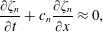 $$\begin{eqnarray}\frac{\unicode[STIX]{x2202}\unicode[STIX]{x1D701}_{n}}{\unicode[STIX]{x2202}t}+c_{n}\frac{\unicode[STIX]{x2202}\unicode[STIX]{x1D701}_{n}}{\unicode[STIX]{x2202}x}\approx 0,\end{eqnarray}$$
the final approximate expression for
 $\unicode[STIX]{x1D6EC}_{n}$
is
$\unicode[STIX]{x1D6EC}_{n}$
is
 $$\begin{eqnarray}\unicode[STIX]{x1D6EC}_{n}S_{n}\approx c_{n}\int _{-h}^{0}u\frac{\unicode[STIX]{x2202}\unicode[STIX]{x1D719}_{n}}{\unicode[STIX]{x2202}z}\,\text{d}z.\end{eqnarray}$$
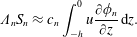
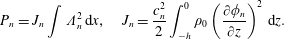
With the aid of this mode decomposition technique (2.30), the amplitude
 $\unicode[STIX]{x1D6EC}_{n}$
of each mode can be easily obtained from the output of the MITgcm. Further, the energy budget of each can also be obtained. Confining attention to linear long-wave theory, see Gill (Reference Gill1982) for instance, the domain-integrated available potential energy (APE) in each mode is
$\unicode[STIX]{x1D6EC}_{n}$
of each mode can be easily obtained from the output of the MITgcm. Further, the energy budget of each can also be obtained. Confining attention to linear long-wave theory, see Gill (Reference Gill1982) for instance, the domain-integrated available potential energy (APE) in each mode is
 $$\begin{eqnarray}P_{n}=\int \int \frac{1}{2}\unicode[STIX]{x1D70C}_{0}N^{2}\unicode[STIX]{x1D701}_{n}^{2}\,\text{d}x\,\text{d}z.\end{eqnarray}$$
Again invoking the Boussinesq approximation, and also considering (2.20), (2.21), (2.23), this can be rewritten in an alternative and more convenient form,
 $$\begin{eqnarray}P_{n}=J_{n}\int \unicode[STIX]{x1D6EC}_{n}^{2}\,\text{d}x,\quad J_{n}=\frac{c_{n}^{2}}{2}\int _{-h}^{0}\unicode[STIX]{x1D70C}_{0}\left(\frac{\unicode[STIX]{x2202}\unicode[STIX]{x1D719}_{n}}{\unicode[STIX]{x2202}z}\right)^{2}\,\text{d}z.\end{eqnarray}$$
Note that the modal functions
 $\unicode[STIX]{x1D719}_{n}$
and speed
$\unicode[STIX]{x1D719}_{n}$
and speed
 $c_{n}$
also contain a slow
$c_{n}$
also contain a slow
 $x$
-dependence, but that is suppressed here at the leading order. In the same slowly varying environment, the velocities in each internal wave mode can be obtained as follows,
$x$
-dependence, but that is suppressed here at the leading order. In the same slowly varying environment, the velocities in each internal wave mode can be obtained as follows,
 $$\begin{eqnarray}\displaystyle & \displaystyle u_{n}(x,z,t)=c_{n}\frac{\unicode[STIX]{x2202}\unicode[STIX]{x1D719}_{n}(z)}{\unicode[STIX]{x2202}z}\unicode[STIX]{x1D6EC}_{n}(x,t), & \displaystyle\end{eqnarray}$$
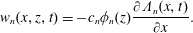 $$\begin{eqnarray}\displaystyle & \displaystyle w_{n}(x,z,t)=-c_{n}\unicode[STIX]{x1D719}_{n}(z)\frac{\unicode[STIX]{x2202}\unicode[STIX]{x1D6EC}_{n}(x,t)}{\unicode[STIX]{x2202}x}. & \displaystyle\end{eqnarray}$$
Then the domain-integrated kinetic energy (KE) in each mode is
 $$\begin{eqnarray}K_{n}=\int \int \frac{1}{2}\unicode[STIX]{x1D70C}_{0}(u_{n}^{2}+w_{n}^{2})\,\text{d}x\text{d}z\approx \int \int \frac{1}{2}\unicode[STIX]{x1D70C}_{0}u_{n}^{2}\,\text{d}x\,\text{d}z=J_{n}\int \unicode[STIX]{x1D6EC}_{n}^{2}\,\text{d}x,\end{eqnarray}$$
as in the long-wave limit used here
 $w_{n}\ll u_{n}$
. As expected, ‘equipartition of energy’ holds here and the total energy can be found as
$w_{n}\ll u_{n}$
. As expected, ‘equipartition of energy’ holds here and the total energy can be found as
 $E_{n}=2K_{n}=2P_{n}$
. Hence it is sufficient to calculate either
$E_{n}=2K_{n}=2P_{n}$
. Hence it is sufficient to calculate either
 $K_{n}$
or
$K_{n}$
or
 $P_{n}$
. Further, It is clear that due to the orthogonality of the modes the total kinetic energy and total potential energy are
$P_{n}$
. Further, It is clear that due to the orthogonality of the modes the total kinetic energy and total potential energy are
 $$\begin{eqnarray}K=\mathop{\sum }_{n}K_{n},\quad P=\mathop{\sum }_{n}P_{n}.\end{eqnarray}$$
3 Three-layer fluid system
It is well known that a three-layer fluid system is the simplest model that can support mode-2 waves, see Yih (Reference Yih1960). Indeed, three-layer density structures have been observed in the ocean, see Yang et al. (Reference Yang, Fang, Tang and Ramp2010) for instance. Hence a three-layer ocean model is used here to investigate the dynamics of mode-2 internal solitary waves. We assume that
 $$\begin{eqnarray}\unicode[STIX]{x1D70C}_{0}(z)=(\unicode[STIX]{x1D70C}_{2}+\unicode[STIX]{x0394}\unicode[STIX]{x1D70C})\unicode[STIX]{x1D6E9}(-z-h_{1}-h_{2})+\unicode[STIX]{x1D70C}_{2}\unicode[STIX]{x1D6E9}(-z-h_{1})\unicode[STIX]{x1D6E9}(z+h_{1}+h_{2})+(\unicode[STIX]{x1D70C}_{2}-\unicode[STIX]{x0394}\unicode[STIX]{x1D70C})\unicode[STIX]{x1D6E9}(z+h_{1}),\end{eqnarray}$$
where
 $\unicode[STIX]{x1D70C}_{2}$
is the density of the middle layer, and the density difference
$\unicode[STIX]{x1D70C}_{2}$
is the density of the middle layer, and the density difference
 $\unicode[STIX]{x0394}\unicode[STIX]{x1D70C}>0$
;
$\unicode[STIX]{x0394}\unicode[STIX]{x1D70C}>0$
;
 $h_{1}$
,
$h_{1}$
,
 $h_{2}$
and
$h_{2}$
and
 $h_{3}$
are the thicknesses of the three layers from top to bottom respectively and
$h_{3}$
are the thicknesses of the three layers from top to bottom respectively and
 $\unicode[STIX]{x1D6E9}(\cdot )$
is the Heaviside function. Note that with this piece-wise constant density field only two of the infinite set of modes can be found, namely mode-1 and mode-2; the remaining modes are confined to the two interfaces, and cannot be found explicitly with this density profile. In principle the densities of these three layers can take any reasonable values depending on the specific circumstances, but here to illustrate the dynamics, we choose one special case in which the density of the middle layer is exactly the mean value of that in the upper layer and bottom layer. From (2.15), (2.16) the modal function is given by
$\unicode[STIX]{x1D6E9}(\cdot )$
is the Heaviside function. Note that with this piece-wise constant density field only two of the infinite set of modes can be found, namely mode-1 and mode-2; the remaining modes are confined to the two interfaces, and cannot be found explicitly with this density profile. In principle the densities of these three layers can take any reasonable values depending on the specific circumstances, but here to illustrate the dynamics, we choose one special case in which the density of the middle layer is exactly the mean value of that in the upper layer and bottom layer. From (2.15), (2.16) the modal function is given by
 $$\begin{eqnarray}\displaystyle \left.\begin{array}{@{}c@{}}\displaystyle \unicode[STIX]{x1D719}=-A_{1}\frac{z}{h_{1}},\quad -h_{1}\leqslant z\leqslant 0,\\ \displaystyle \unicode[STIX]{x1D719}=A_{1}\frac{z+h_{1}+h_{2}}{h_{2}}-A_{2}\frac{z+h_{1}}{h_{2}},\quad -h_{1}-h_{2}<z<-h_{1},\\ \displaystyle \unicode[STIX]{x1D719}=A_{2}\frac{z+h}{h_{3}},\quad -h\leqslant z\leqslant -h_{1}-h_{2}.\end{array}\right\} & & \displaystyle\end{eqnarray}$$
Note that
 $\unicode[STIX]{x1D719}=A_{1}$
at the upper interface
$\unicode[STIX]{x1D719}=A_{1}$
at the upper interface
 $z=-h_{1}$
, and
$z=-h_{1}$
, and
 $\unicode[STIX]{x1D719}=A_{2}$
at the lower interface
$\unicode[STIX]{x1D719}=A_{2}$
at the lower interface
 $z=-h_{1}-h_{2}$
. The solution is normalised by
$z=-h_{1}-h_{2}$
. The solution is normalised by
 $\max [|\unicode[STIX]{x1D719}|]=1$
, so that
$\max [|\unicode[STIX]{x1D719}|]=1$
, so that
 $\max [|A_{1}|,|A_{2}|]=1$
, and without loss of generality, we require that
$\max [|A_{1}|,|A_{2}|]=1$
, and without loss of generality, we require that
 $0<A_{1}\leqslant 1$
. The speed
$0<A_{1}\leqslant 1$
. The speed
 $c$
is now found by noting that at
$c$
is now found by noting that at
 $z=-h_{1},-h_{1}-h_{2}$
,
$z=-h_{1},-h_{1}-h_{2}$
,
 $\unicode[STIX]{x1D719}_{z}$
is discontinuous and
$\unicode[STIX]{x1D719}_{z}$
is discontinuous and
 $\unicode[STIX]{x1D70C}_{0z}$
consists of two
$\unicode[STIX]{x1D70C}_{0z}$
consists of two
 $\unicode[STIX]{x1D6FF}$
-functions. Integrating the modal equation (2.15) across each interface leads to
$\unicode[STIX]{x1D6FF}$
-functions. Integrating the modal equation (2.15) across each interface leads to
 $$\begin{eqnarray}c^{2}[\unicode[STIX]{x1D719}_{z}]_{-}^{+}+g^{\prime }\unicode[STIX]{x1D719}=0,\quad g^{\prime }=g\frac{\unicode[STIX]{x0394}\unicode[STIX]{x1D70C}}{\unicode[STIX]{x1D70C}_{2}},\end{eqnarray}$$
where
 $[\cdot ]_{-}^{+}$
is the difference between above and below each interface. Note that these jump conditions represent continuity of total pressure across each interface. Hence the speed
$[\cdot ]_{-}^{+}$
is the difference between above and below each interface. Note that these jump conditions represent continuity of total pressure across each interface. Hence the speed
 $c$
is found from the
$c$
is found from the
 $2\times 2$
eigenvalue problem,
$2\times 2$
eigenvalue problem,
 $$\begin{eqnarray}\displaystyle \left.\begin{array}{@{}c@{}}\displaystyle c^{2}\left\{A_{1}\left(\frac{1}{h_{1}}+\frac{1}{h_{2}}\right)-\frac{A_{2}}{h_{2}}\right\}-g^{\prime }A_{1}=0,\\ \displaystyle c^{2}\left\{A_{2}\left(\frac{1}{h_{2}}+\frac{1}{h_{3}}\right)-\frac{A_{1}}{h_{2}}\right\}-g^{\prime }A_{2}=0,\end{array}\right\} & & \displaystyle\end{eqnarray}$$
 $$\begin{eqnarray}\frac{2g^{\prime }}{c^{2}}=\left(\frac{1}{h_{1}}+\frac{2}{h_{2}}+\frac{1}{h_{3}}\right)\mp \left\{\left(\frac{1}{h_{1}}-\frac{1}{h_{3}}\right)^{2}+\frac{4}{h_{2}^{2}}\right\}^{1/2}.\end{eqnarray}$$
The signs
 $\mp$
correspond to mode-1 and mode-2 respectively, so that, as expected
$\mp$
correspond to mode-1 and mode-2 respectively, so that, as expected
 $c_{1}>c_{2}$
. It then follows that
$c_{1}>c_{2}$
. It then follows that
 $$\begin{eqnarray}\frac{A_{1}}{A_{2}}=R=H\pm (H^{2}+1)^{1/2},\quad \frac{A_{2}}{A_{1}}=\frac{1}{R}=-H\pm (H^{2}+1)^{1/2},\quad H=\frac{h_{2}}{2}\left(\frac{1}{h_{3}}-\frac{1}{h_{1}}\right).\end{eqnarray}$$
Hence
 $R>0({<}0)$
for mode-1 and mode-2 respectively, so that, as expected, mode-1 has no internal zeros, and mode-2 has just one internal zero. Thus both the phase speed and internal zero criteria for distinguishing between mode-1 and mode-2 are valid here. Also, for mode-1,
$R>0({<}0)$
for mode-1 and mode-2 respectively, so that, as expected, mode-1 has no internal zeros, and mode-2 has just one internal zero. Thus both the phase speed and internal zero criteria for distinguishing between mode-1 and mode-2 are valid here. Also, for mode-1,
 $R>1({<}1)$
according as
$R>1({<}1)$
according as
 $H>0({<}0)$
, that is
$H>0({<}0)$
, that is
 $h_{1}/h_{3}>1({<}1)$
, while for mode-2
$h_{1}/h_{3}>1({<}1)$
, while for mode-2
 $|R|<1({>}1)$
according as
$|R|<1({>}1)$
according as
 $H>0({<}0)$
. Note that
$H>0({<}0)$
. Note that
 $$\begin{eqnarray}\frac{g^{\prime }h_{2}}{c^{2}}=\frac{h_{2}}{h_{1}}+1+H\mp (H^{2}+1)^{1/2}=\frac{h_{2}}{h_{3}}+1-H\mp (H^{2}+1)^{1/2}.\end{eqnarray}$$
Then the coefficient
 $\unicode[STIX]{x1D707}$
(2.17) is given by
$\unicode[STIX]{x1D707}$
(2.17) is given by
 $$\begin{eqnarray}I\unicode[STIX]{x1D707}=3c^{2}\left\{-\frac{A_{1}^{3}}{h_{1}^{2}}+\frac{A_{2}^{3}}{h_{3}^{2}}+\frac{(A_{1}-A_{2})^{3}}{h_{2}^{2}}\right\},\quad I=2c\left\{\frac{A_{1}^{2}}{h_{1}}+\frac{A_{2}^{2}}{h_{3}}+\frac{(A_{1}-A_{2})^{2}}{h_{2}}\right\}.\end{eqnarray}$$
Substituting the expressions (3.6) into (3.8) we get that
 $$\begin{eqnarray}\unicode[STIX]{x1D707}=\frac{3cA_{2}}{2h_{2}}\frac{\unicode[STIX]{x1D6FA}}{\unicode[STIX]{x1D6F1}},\quad \unicode[STIX]{x1D6FA}=-\frac{h_{2}^{2}}{h_{1}^{2}}R^{3}+\frac{h_{2}^{2}}{h_{3}^{2}}+(R-1)^{3},\quad \unicode[STIX]{x1D6F1}=\frac{h_{2}}{h_{1}}R^{2}+\frac{h_{2}}{h_{3}}+(R-1)^{2}.\end{eqnarray}$$
Our main concern is how these expressions vary as the lower-layer depth
 $h_{3}$
decreases. Since for all the cases we consider, in the deep water
$h_{3}$
decreases. Since for all the cases we consider, in the deep water
 $h_{1}=h_{3}$
, we can assume that
$h_{1}=h_{3}$
, we can assume that
 $h_{1}>h_{3}$
as the waves propagate up the slope. In this case
$h_{1}>h_{3}$
as the waves propagate up the slope. In this case
 $H>0$
,
$H>0$
,
 $R>1$
for mode-1 and
$R>1$
for mode-1 and
 $-1<R<0$
for mode-2, so that recalling the convention that
$-1<R<0$
for mode-2, so that recalling the convention that
 $A_{1}>0$
,
$A_{1}>0$
,
 $A_{1}=1,0<A_{2}<1$
for mode-1 and
$A_{1}=1,0<A_{2}<1$
for mode-1 and
 $0<A_{1}<1,A_{2}=-1$
for mode-2. A useful approximation is
$0<A_{1}<1,A_{2}=-1$
for mode-2. A useful approximation is
 $h_{2}\ll h_{1,3}$
when
$h_{2}\ll h_{1,3}$
when
 $H\rightarrow 0$
and so
$H\rightarrow 0$
and so
 $$\begin{eqnarray}\displaystyle \left.\begin{array}{@{}ll@{}}\displaystyle \text{mode-1:}\quad & \displaystyle c^{2}=2g^{\prime }h_{1}h_{3}/(h_{1}+h_{3}),\quad A_{1}=A_{2}=1,\quad \unicode[STIX]{x1D707}=\frac{3c(h_{1}-h_{3})}{2h_{1}h_{3}},\\ \displaystyle \text{mode-2:}\quad & \displaystyle c^{2}=g^{\prime }h_{2}/2,\quad A_{1}=-A_{2}=1,\quad \unicode[STIX]{x1D707}=\frac{3c}{2h_{2}}.\end{array}\right\} & & \displaystyle\end{eqnarray}$$
Another useful limit is
 $h_{3}\rightarrow 0$
when
$h_{3}\rightarrow 0$
when
 $H\rightarrow +\infty$
, and so
$H\rightarrow +\infty$
, and so
 $$\begin{eqnarray}\displaystyle \left.\begin{array}{@{}ll@{}}\displaystyle \text{mode-1:}\quad & \displaystyle c^{2}=g^{\prime }h_{1}h_{2}/(h_{1}+h_{2}),\quad A_{1}=1,A_{2}=0,\quad \unicode[STIX]{x1D707}=\frac{3c(h_{1}-h_{2})}{2h_{1}h_{2}},\\ \displaystyle \text{mode-2:}\quad & \displaystyle c^{2}\approx g^{\prime }h_{3},\quad A_{1}=0,A_{2}=-1,\quad \unicode[STIX]{x1D707}=-\frac{3c}{2h_{3}}.\end{array}\right\} & & \displaystyle\end{eqnarray}$$
Note that in the deep water,
 $h_{1}=h_{3}$
,
$h_{1}=h_{3}$
,
 $H=0$
,
$H=0$
,
 $R=\pm 1$
,
$R=\pm 1$
,
 $A_{1}=A_{2}=1$
for mode-1,
$A_{1}=A_{2}=1$
for mode-1,
 $A_{1}=-A_{2}=1$
for mode-2 and
$A_{1}=-A_{2}=1$
for mode-2 and
 $$\begin{eqnarray}\left.\begin{array}{@{}ll@{}}\displaystyle \text{mode-1:}\quad & \displaystyle c^{2}=g^{\prime }h_{1},\quad \unicode[STIX]{x1D707}=0,\\ \displaystyle \text{mode-2:}\quad & \displaystyle c^{2}=\frac{g^{\prime }h_{1}h_{2}}{(2h_{1}+h_{2})},\quad \unicode[STIX]{x1D707}=\frac{3c(2h_{1}-h_{2})}{2h_{1}h_{2}}.\end{array}\right\}\end{eqnarray}$$
These expressions show that for mode-1
 $\unicode[STIX]{x1D707}\geqslant 0$
when
$\unicode[STIX]{x1D707}\geqslant 0$
when
 $h_{1}\geqslant h_{3}$
in the limit
$h_{1}\geqslant h_{3}$
in the limit
 $h_{2}\ll h_{1,3}$
,
$h_{2}\ll h_{1,3}$
,
 $\unicode[STIX]{x1D707}\geqslant 0$
when
$\unicode[STIX]{x1D707}\geqslant 0$
when
 $h_{1}\geqslant h_{2}$
in the limit
$h_{1}\geqslant h_{2}$
in the limit
 $h_{3}\rightarrow 0$
and
$h_{3}\rightarrow 0$
and
 $\unicode[STIX]{x1D707}=0$
when
$\unicode[STIX]{x1D707}=0$
when
 $h_{1}=h_{3}$
. For mode-2,
$h_{1}=h_{3}$
. For mode-2,
 $\unicode[STIX]{x1D707}>0$
in the limit
$\unicode[STIX]{x1D707}>0$
in the limit
 $h_{2}\ll h_{1,3}$
, while
$h_{2}\ll h_{1,3}$
, while
 $\unicode[STIX]{x1D707}<0$
in the limit
$\unicode[STIX]{x1D707}<0$
in the limit
 $h_{3}\rightarrow 0$
, but
$h_{3}\rightarrow 0$
, but
 $\unicode[STIX]{x1D707}\geqslant 0$
when
$\unicode[STIX]{x1D707}\geqslant 0$
when
 $2h_{1}\geqslant h_{2}$
for the case
$2h_{1}\geqslant h_{2}$
for the case
 $h_{1}=h_{3}$
. In general the sign of
$h_{1}=h_{3}$
. In general the sign of
 $\unicode[STIX]{x1D707}$
is determined by the sign of
$\unicode[STIX]{x1D707}$
is determined by the sign of
 $A_{2}\unicode[STIX]{x1D6FA}$
, which is defined in (3.9), and in particular
$A_{2}\unicode[STIX]{x1D6FA}$
, which is defined in (3.9), and in particular
 $\unicode[STIX]{x1D707}=0$
when
$\unicode[STIX]{x1D707}=0$
when
 $$\begin{eqnarray}\frac{h_{2}}{h_{1}}(1-R^{3})=-2H\pm \{4H^{2}R^{3}+(1-R^{3})(1-R)^{3}\}^{1/2},\end{eqnarray}$$
which defines the curves in the
 $h_{2}/h_{1},h_{2}/h_{3}$
plane where
$h_{2}/h_{1},h_{2}/h_{3}$
plane where
 $\unicode[STIX]{x1D707}=0$
. Recalling that
$\unicode[STIX]{x1D707}=0$
. Recalling that
 $h_{1}>h_{3}$
,
$h_{1}>h_{3}$
,
 $H>0$
, for mode-1
$H>0$
, for mode-1
 $R>1$
, the discriminant is positive and only the lower sign can be taken. In the limit
$R>1$
, the discriminant is positive and only the lower sign can be taken. In the limit
 $h_{1}\rightarrow h_{3}$
, this yields
$h_{1}\rightarrow h_{3}$
, this yields
 $h_{2}/h_{1}\rightarrow 4/3$
, so that there is a change of sign at this point just above the line
$h_{2}/h_{1}\rightarrow 4/3$
, so that there is a change of sign at this point just above the line
 $h_{2}/h_{1}=h_{2}/h_{3}$
. For mode-2,
$h_{2}/h_{1}=h_{2}/h_{3}$
. For mode-2,
 $-1<R<0$
, the discriminant is positive only when
$-1<R<0$
, the discriminant is positive only when
 $H$
is large enough, and then the upper sign must be chosen. In the limit
$H$
is large enough, and then the upper sign must be chosen. In the limit
 $h_{1}\rightarrow h_{3}$
, this yields
$h_{1}\rightarrow h_{3}$
, this yields
 $h_{2}/h_{1}\rightarrow 2$
. The outcome for the sign of
$h_{2}/h_{1}\rightarrow 2$
. The outcome for the sign of
 $\unicode[STIX]{x1D707}$
is shown in figure 1. In practice,
$\unicode[STIX]{x1D707}$
is shown in figure 1. In practice,
 $h_{1}$
and
$h_{1}$
and
 $h_{2}$
are constants, and so
$h_{2}$
are constants, and so
 $H_{1}=h_{2}/h_{1}$
is constant when the internal solitary wave propagates shoreward, while
$H_{1}=h_{2}/h_{1}$
is constant when the internal solitary wave propagates shoreward, while
 $H_{3}=h_{2}/h_{3}$
is the only variable to change as
$H_{3}=h_{2}/h_{3}$
is the only variable to change as
 $h_{3}$
changes. Hence we consider two cases: a polarity change and no polarity change, which will be shown in the next section.
$h_{3}$
changes. Hence we consider two cases: a polarity change and no polarity change, which will be shown in the next section.

Figure 1. Plot of the nonlinear coefficient
 $\unicode[STIX]{x1D707}$
(3.9) for mode-1 (a) and mode-2 (b). Shaded areas show negative value,
$\unicode[STIX]{x1D707}$
(3.9) for mode-1 (a) and mode-2 (b). Shaded areas show negative value,
 $\unicode[STIX]{x1D707}<0$
. Labels are
$\unicode[STIX]{x1D707}<0$
. Labels are
 $H_{1}=h_{2}/h_{1},H_{3}=h_{2}/h_{3}$
.
$H_{1}=h_{2}/h_{1},H_{3}=h_{2}/h_{3}$
.
4 From one three-layer system to another
As discussed in § 1 the vKdV equation (2.1) and various extensions have been extensively used to model the evolution of internal waves over topography in the coastal oceans. For instance, Grimshaw et al. (Reference Grimshaw, Pelinovsky, Talipova and Kurkin2004) used an extended vKdV equation to study the transformation of a mode-1 internal solitary wave as it evolves over three representative continental shelves; Holloway, Pelinovsky & Talipova (Reference Holloway, Pelinovsky and Talipova1999) studied the evolution of internal tides when they propagate shoreward with a generalised KdV equation, which considers the combined effect of both quadratic and cubic nonlinearity, the Earth’s rotation, and frictional dissipation. However, the investigation of the evolution and propagation of mode-2 internal solitary waves over a slope seems to be very rare. Indeed, the only comparable studies we are aware of are those by Guo & Chen (Reference Guo and Chen2012) and Terletska et al. (Reference Terletska, Jung, Talipova, Maderich, Brovchenko and Grimshaw2016), and we will make comparisons and discussions of these works in the summary, § 6.
We consider a three-layer system, in which the background current is zero and the density variations across each interface are the same, that is, the density is
 $\unicode[STIX]{x1D70C}_{2}-\unicode[STIX]{x0394}\unicode[STIX]{x1D70C}$
,
$\unicode[STIX]{x1D70C}_{2}-\unicode[STIX]{x0394}\unicode[STIX]{x1D70C}$
,
 $\unicode[STIX]{x1D70C}_{2}$
and
$\unicode[STIX]{x1D70C}_{2}$
and
 $\unicode[STIX]{x1D70C}_{2}+\unicode[STIX]{x0394}\unicode[STIX]{x1D70C}$
respectively from top to bottom, where
$\unicode[STIX]{x1D70C}_{2}+\unicode[STIX]{x0394}\unicode[STIX]{x1D70C}$
respectively from top to bottom, where
 $\unicode[STIX]{x0394}\unicode[STIX]{x1D70C}>0$
, exactly as listed in § 3. Two configurations are investigated, both of which keep the thicknesses of the upper and middle layer as constants, that is,
$\unicode[STIX]{x0394}\unicode[STIX]{x1D70C}>0$
, exactly as listed in § 3. Two configurations are investigated, both of which keep the thicknesses of the upper and middle layer as constants, that is,
 $h_{1}=200~\text{m}$
and
$h_{1}=200~\text{m}$
and
 $h_{2}=100~\text{m}$
, and only the bottom layer
$h_{2}=100~\text{m}$
, and only the bottom layer
 $h_{3}$
varies as the waves move into shallow water. To model a realistic ocean situation, the idealised bathymetry used here has a typical slope-shelf structure, see figure 2. Initially in the deep water, the bottom layer
$h_{3}$
varies as the waves move into shallow water. To model a realistic ocean situation, the idealised bathymetry used here has a typical slope-shelf structure, see figure 2. Initially in the deep water, the bottom layer
 $h_{3}=200~\text{m}$
, then decreases along the linearly varying slope to
$h_{3}=200~\text{m}$
, then decreases along the linearly varying slope to
 $h_{3}=50~\text{m}$
(labelled as EXP1) or
$h_{3}=50~\text{m}$
(labelled as EXP1) or
 $h_{3}=60~\text{m}$
(labelled as EXP2) respectively onto the shelf. As a consequence, the thickness ratio
$h_{3}=60~\text{m}$
(labelled as EXP2) respectively onto the shelf. As a consequence, the thickness ratio
 $H_{1}=h_{2}/h_{1}=0.5$
is a constant, while
$H_{1}=h_{2}/h_{1}=0.5$
is a constant, while
 $H_{3}=h_{2}/h_{3}$
adjusts from
$H_{3}=h_{2}/h_{3}$
adjusts from
 $H_{3}=0.5$
in the deep water to
$H_{3}=0.5$
in the deep water to
 $H_{3}=2$
and
$H_{3}=2$
and
 $H_{3}=1.67$
respectively on the shelf. Although in these two cases EXP1 and EXP2, this 10 m thickness difference on the shelf may seem small, especially when compared with the total water depth (500 m), the corresponding dynamics can be completely distinguished from each other. When
$H_{3}=1.67$
respectively on the shelf. Although in these two cases EXP1 and EXP2, this 10 m thickness difference on the shelf may seem small, especially when compared with the total water depth (500 m), the corresponding dynamics can be completely distinguished from each other. When
 $h_{3}=50~\text{m}$
(
$h_{3}=50~\text{m}$
(
 $H_{3}=2$
) on the shelf, referring to figure 1, the nonlinear coefficient
$H_{3}=2$
) on the shelf, referring to figure 1, the nonlinear coefficient
 $\unicode[STIX]{x1D707}$
in (2.1) (and so also
$\unicode[STIX]{x1D707}$
in (2.1) (and so also
 $\unicode[STIX]{x1D6FC}$
in (2.7)) is negative, opposite from the positive value in the deep water, which indicates there must be a critical point on the slope, where
$\unicode[STIX]{x1D6FC}$
in (2.7)) is negative, opposite from the positive value in the deep water, which indicates there must be a critical point on the slope, where
 $\unicode[STIX]{x1D6FC}=0$
, and passing through that point, the initial convex wave (
$\unicode[STIX]{x1D6FC}=0$
, and passing through that point, the initial convex wave (
 $\unicode[STIX]{x1D707}>0$
) inverses its polarity and turns into a concave wave (
$\unicode[STIX]{x1D707}>0$
) inverses its polarity and turns into a concave wave (
 $\unicode[STIX]{x1D707}<0$
), that is, there is a polarity change. In contrast, the other case EXP2 is in a different regime, since
$\unicode[STIX]{x1D707}<0$
), that is, there is a polarity change. In contrast, the other case EXP2 is in a different regime, since
 $\unicode[STIX]{x1D707}$
preserves its sign,
$\unicode[STIX]{x1D707}$
preserves its sign,
 $\unicode[STIX]{x1D707}>0$
, so there is no polarity change. Our numerical simulations are performed in the transformed space on (2.7), using a pseudo-spectral method based on a Fourier interpolant, see Boyd (Reference Boyd2001) and Weideman & Reddy (Reference Weideman and Reddy2000) for details. The ‘spatial’ resolution is 0.5 s in
$\unicode[STIX]{x1D707}>0$
, so there is no polarity change. Our numerical simulations are performed in the transformed space on (2.7), using a pseudo-spectral method based on a Fourier interpolant, see Boyd (Reference Boyd2001) and Weideman & Reddy (Reference Weideman and Reddy2000) for details. The ‘spatial’ resolution is 0.5 s in
 $X$
, while the ‘temporal’ resolution is
$X$
, while the ‘temporal’ resolution is
 $0.08~\text{s}^{3}$
in
$0.08~\text{s}^{3}$
in
 $\unicode[STIX]{x1D70F}$
, and finally the outcome is transformed back to the physical space.
$\unicode[STIX]{x1D70F}$
, and finally the outcome is transformed back to the physical space.

Figure 2. Coefficients of the vKdV equation (2.3) for mode-2, together with the corresponding bathymetry and density layers. (a) The EXP1, in which there is a polarity change (
 $h_{3}=50~\text{m}$
in the shallow water); (b) the EXP2, in which there is no polarity change (
$h_{3}=50~\text{m}$
in the shallow water); (b) the EXP2, in which there is no polarity change (
 $h_{3}=60~\text{m}$
in the shallow water). The dark dash-dotted line indicates where
$h_{3}=60~\text{m}$
in the shallow water). The dark dash-dotted line indicates where
 $\unicode[STIX]{x1D708}=0$
, while the grey dashed lines denote the two interfaces. Note that in the EXP1, the critical point (
$\unicode[STIX]{x1D708}=0$
, while the grey dashed lines denote the two interfaces. Note that in the EXP1, the critical point (
 $\unicode[STIX]{x1D708}=0$
) locates at approximately
$\unicode[STIX]{x1D708}=0$
) locates at approximately
 $x=1.8\times 10^{5}~\text{m}$
, just in the vicinity of the end of the slope at
$x=1.8\times 10^{5}~\text{m}$
, just in the vicinity of the end of the slope at
 $x=1.82\times 10^{5}~\text{m}$
.
$x=1.82\times 10^{5}~\text{m}$
.
In the shoaling process, as the depth decreases the linear magnification factor
 $Q$
increases, while the linear dispersive coefficient
$Q$
increases, while the linear dispersive coefficient
 $\unicode[STIX]{x1D6FF}$
decreases, see figure 2. In particular, the decrease in
$\unicode[STIX]{x1D6FF}$
decreases, see figure 2. In particular, the decrease in
 $\unicode[STIX]{x1D6FF}$
consequently enhances the effect of nonlinearity as the wave propagates shoreward, which can subsequently change the waveform.
$\unicode[STIX]{x1D6FF}$
consequently enhances the effect of nonlinearity as the wave propagates shoreward, which can subsequently change the waveform.

Figure 3. The amplitudes of the mode-2 internal solitary waves in simulations of the vKdV equation (2.7). Note that the results are transformed back to the physical space from the calculation space. (a,c,e) The EXP1, and the critical point is at approximately
 $x=1.8\times 10^{5}~\text{m}$
; (b,d,f) the EXP2. One point worth mentioning is that in order to emphasise the waveform, the horizontal scale changes, especially from the top to the middle panel.
$x=1.8\times 10^{5}~\text{m}$
; (b,d,f) the EXP2. One point worth mentioning is that in order to emphasise the waveform, the horizontal scale changes, especially from the top to the middle panel.
The deformation scenarios of the EXP1 and EXP2 are depicted in figure 3. In the EXP1, a single convex wave with an initial amplitude of 18 m propagates shoreward, and as expected, the evolution is adiabatic without significant change until it reaches the critical point. Prior to the critical point, the vKdV theory predicts that the amplitude decreases as
 $\unicode[STIX]{x1D6FC}^{1/3}$
reduces, where
$\unicode[STIX]{x1D6FC}^{1/3}$
reduces, where
 $\unicode[STIX]{x1D6FC}$
is the nonlinear coefficient in (2.7). Then, approaching the critical point, this slowly varying solitary wave generates a trailing shelf of the opposite polarity, and this combination passes through the critical point. Thereafter as
$\unicode[STIX]{x1D6FC}$
is the nonlinear coefficient in (2.7). Then, approaching the critical point, this slowly varying solitary wave generates a trailing shelf of the opposite polarity, and this combination passes through the critical point. Thereafter as
 $\unicode[STIX]{x1D6FC}$
becomes negative, this disturbance forms into a leading positive rarefaction wave at whose trailing edge an incipient jump is resolved by an undular bore whose leading component is a solitary wave train of negative polarity, see Grimshaw & Yuan (Reference Grimshaw and Yuan2016). The case with no polarity change EXP2 is distinct, as
$\unicode[STIX]{x1D6FC}$
becomes negative, this disturbance forms into a leading positive rarefaction wave at whose trailing edge an incipient jump is resolved by an undular bore whose leading component is a solitary wave train of negative polarity, see Grimshaw & Yuan (Reference Grimshaw and Yuan2016). The case with no polarity change EXP2 is distinct, as
 $\unicode[STIX]{x1D6FC}$
decreases, the mass of the solitary wave increases as
$\unicode[STIX]{x1D6FC}$
decreases, the mass of the solitary wave increases as
 $\unicode[STIX]{x1D6FC}^{-1/3}$
, and this generates a negative trailing pedestal to conserve the total mass. But then instead of passing through a critical point,
$\unicode[STIX]{x1D6FC}^{-1/3}$
, and this generates a negative trailing pedestal to conserve the total mass. But then instead of passing through a critical point,
 $\unicode[STIX]{x1D6FC}$
approaches a constant value on the shelf, and hence the leading convex wave continues steadily, while new internal solitary waves of small amplitude and negative polarity form from the trailing pedestal.
$\unicode[STIX]{x1D6FC}$
approaches a constant value on the shelf, and hence the leading convex wave continues steadily, while new internal solitary waves of small amplitude and negative polarity form from the trailing pedestal.
Next, we compare these results to simulations using a primitive equation model, the MIT general circulation model (MITgcm), with zero horizontal and vertical Laplacian frictional dissipation, so that formally it solves the incompressible Boussinesq equations with fully nonlinear and non-hydrostatic terms, employed here in a two-dimensional configuration. This model uses a finite-volume method and has been successfully used to study internal waves in the ocean, such as Vlasenko et al. (Reference Vlasenko, Stashchuk, Guo and Chen2010) and Guo & Chen (Reference Guo and Chen2012). For details of the MITgcm model, refer to Marshall et al. (Reference Marshall, Adcroft, Hill, Perelman and Heisey1997). Our model domain and bathymetry are the same as those in the vKdV equation. The spatial steps are 1 and 50 m in the vertical and horizontal direction respectively, and using a similar method to that introduced in Guo & Chen (Reference Guo and Chen2012), two boundary layers, where the resolution exponentially decreases from 50 to
 $2.5\times 10^{5}~\text{m}$
, are added at the ends of domain to suppress any reflections. In addition, considering the time scale of the waves, we set the time step to be 4 s. The background temperature is uniform in this model,
$2.5\times 10^{5}~\text{m}$
, are added at the ends of domain to suppress any reflections. In addition, considering the time scale of the waves, we set the time step to be 4 s. The background temperature is uniform in this model,
 $25\,^{\circ }$
C, while the salinity is 5, 20 and 35 PSU respectively for the three layers. Neglecting the pressure deviation in the fluid, the corresponding densities can be achieved by the equation of state at atmospheric pressure with values of 1000.8, 1012.0 and
$25\,^{\circ }$
C, while the salinity is 5, 20 and 35 PSU respectively for the three layers. Neglecting the pressure deviation in the fluid, the corresponding densities can be achieved by the equation of state at atmospheric pressure with values of 1000.8, 1012.0 and
 $1023.3~\text{kg}~\text{m}^{-3}$
. In addition, to ensure that the model runs smoothly, we invoke a Leith scheme, see Leith (Reference Leith1996), to introduce some viscosity. The KdV-type mode-2 solitary wave is not an exact solution of the Boussinesq equations solved by the MITgcm model, but nevertheless, essentially only some slight modulations are needed. Thus to obtain the initial wave, a preliminary MITgcm model run with the KdV wave as the initial condition is performed. As expected, the final usable stable incident mode-2 waves are followed by some small trailing waves.
$1023.3~\text{kg}~\text{m}^{-3}$
. In addition, to ensure that the model runs smoothly, we invoke a Leith scheme, see Leith (Reference Leith1996), to introduce some viscosity. The KdV-type mode-2 solitary wave is not an exact solution of the Boussinesq equations solved by the MITgcm model, but nevertheless, essentially only some slight modulations are needed. Thus to obtain the initial wave, a preliminary MITgcm model run with the KdV wave as the initial condition is performed. As expected, the final usable stable incident mode-2 waves are followed by some small trailing waves.
Using the modal system (2.15), (2.16), it is found the fluctuation of the interface between the upper and middle layer in the MITgcm model is just the amplitude
 $A$
in the vKdV equation (2.1). Figure 4 shows a comparison between the vKdV and the MITgcm simulations. Here for brevity, only the result of the EXP1 is exhibited. Note that all the coefficients
$A$
in the vKdV equation (2.1). Figure 4 shows a comparison between the vKdV and the MITgcm simulations. Here for brevity, only the result of the EXP1 is exhibited. Note that all the coefficients
 $c,Q,\unicode[STIX]{x1D707},\unicode[STIX]{x1D706}$
in (2.1) have to be solved by numerical methods, and as a result, an interpolation is implemented in the transformation from
$c,Q,\unicode[STIX]{x1D707},\unicode[STIX]{x1D706}$
in (2.1) have to be solved by numerical methods, and as a result, an interpolation is implemented in the transformation from
 $U$
in (2.7) to
$U$
in (2.7) to
 $A$
in (2.3 or 2.1). Nevertheless, considering the very fine resolution (
$A$
in (2.3 or 2.1). Nevertheless, considering the very fine resolution (
 $X:0.5~\text{s}$
,
$X:0.5~\text{s}$
,
 $\unicode[STIX]{x1D70F}:0.08~\text{s}^{3}$
) used in the calculation of (2.7), this transformation can still reach a high accuracy. Despite the fact that the amplitude of the MITgcm result is smaller than that from the vKdV equation, these two have a good agreement. The MITgcm model solves the primitive equation, which can support solutions for all modes, including the mode-1 and mode-2 waves, while the vKdV equation by construction is not able to support mode-1 and mode-2 simultaneously. Hence, in the MITgcm simulations there is a possibility for a generation of mode-1 and higher modes, and energy exchange between modes, which is possibly the reason why a smaller amplitude occurs. In addition, the viscosity and numerical wave breaking and turbulent mixing can be another sink for the energy. Indeed, as analysed in the following results for the energy budget, these may represent a large portion of the lost energy.
$\unicode[STIX]{x1D70F}:0.08~\text{s}^{3}$
) used in the calculation of (2.7), this transformation can still reach a high accuracy. Despite the fact that the amplitude of the MITgcm result is smaller than that from the vKdV equation, these two have a good agreement. The MITgcm model solves the primitive equation, which can support solutions for all modes, including the mode-1 and mode-2 waves, while the vKdV equation by construction is not able to support mode-1 and mode-2 simultaneously. Hence, in the MITgcm simulations there is a possibility for a generation of mode-1 and higher modes, and energy exchange between modes, which is possibly the reason why a smaller amplitude occurs. In addition, the viscosity and numerical wave breaking and turbulent mixing can be another sink for the energy. Indeed, as analysed in the following results for the energy budget, these may represent a large portion of the lost energy.
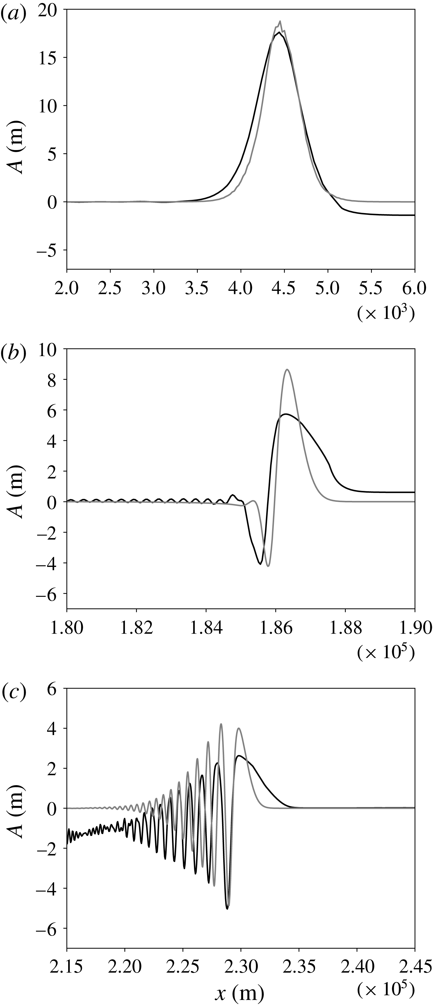
Figure 4. Three representative snapshots of the EXP1 at times
 $t=0,22$
and
$t=0,22$
and
 $30~\text{h}$
(from (a) to (c)) in a three-layer to three-layer system are illustrated. The grey line is the result from the vKdV equation (2.7), but is transformed back to the physical space, while the dark line is the isopycnal line
$30~\text{h}$
(from (a) to (c)) in a three-layer to three-layer system are illustrated. The grey line is the result from the vKdV equation (2.7), but is transformed back to the physical space, while the dark line is the isopycnal line
 $\unicode[STIX]{x1D70C}=\unicode[STIX]{x1D70C}_{2}-\unicode[STIX]{x0394}\unicode[STIX]{x1D70C}=1000.8~\text{kg}~\text{m}^{-3}$
, which is also the interface between the upper and middle layer, captured from the MITgcm model. As the origins of coordinates are not the same, the MITgcm result is shifted in order to make the comparison.
$\unicode[STIX]{x1D70C}=\unicode[STIX]{x1D70C}_{2}-\unicode[STIX]{x0394}\unicode[STIX]{x1D70C}=1000.8~\text{kg}~\text{m}^{-3}$
, which is also the interface between the upper and middle layer, captured from the MITgcm model. As the origins of coordinates are not the same, the MITgcm result is shifted in order to make the comparison.

Figure 5. The MITgcm simulation of the EXP1 in a three-layer to three-layer system. The upper panel (a) is the mode decomposition result for mode-2 internal solitary waves at times
 $t=0,10,21$
and
$t=0,10,21$
and
 $30~\text{h}$
, which are shown by blue, orange, green and red solid lines respectively. The four panels (b) are results for mode-1 at the same times, and are represented by the same coloured lines as that for mode-2. Dark dots indicate the start and the end of the linearly varying slope, respectively. The lowest two panels (c) are snapshots which are bounded by the corresponding dark dashed rectangle.
$30~\text{h}$
, which are shown by blue, orange, green and red solid lines respectively. The four panels (b) are results for mode-1 at the same times, and are represented by the same coloured lines as that for mode-2. Dark dots indicate the start and the end of the linearly varying slope, respectively. The lowest two panels (c) are snapshots which are bounded by the corresponding dark dashed rectangle.
A mode decomposition technique, see (2.30) in § 2, is implemented on the MITgcm result, see figure 5. As expected, the mode-2 wave decomposition result behaves very similar to the evolution based on the vKdV equation (2.7), see figure 3. In the deep water there is a very small mode-1 feature slaved to the main mode-2 wave, as the latter is not quite an exact mode-2 internal solitary wave as given in the KdV theory. However after this mode-2 wave propagates onto the slope, this slaved feature grows into a mode-1 wave train, as energy flows from mode-2 into mode-1. In addition a very small free mode-1 wave is generated which propagates ahead of the main mode-1 wave. The slaved mode-1 wave train accumulates energy gradually during the evolution of the mode-2 wave propagating up the slope, and a leading depression rarefaction forms followed by trailing oscillatory wave trains. Ahead of this slaved component, there is a small freely propagating mode-1 rarefaction. Note that the vKdV theory predicts that nonlinear effects become more significant as the mode-1 wave moves up the slope, see figure 6. Finally, on the flat shelf, the slaved mode-1 wave continues to develop but the freely propagating mode-1 wave can hardly be seen. Importantly, the amplitudes of these mode-1 waves remain much smaller than that of the main mode-2 wave, so the energy transfer is quite small. This can be confirmed from an analysis of the energy budget, see figure 7. Here we use the expressions (2.32), (2.35) for the energy in each mode, consistent with the vKdV theory. But we note that in the fully nonlinear MITgcm simulations, for large amplitude waves this could lead to some significant errors, see Lamb (Reference Lamb2007). Nevertheless, mode-2 waves lose
 $0.68$
TJ (
$0.68$
TJ (
 $\times 10^{12}$
joules) of energy over the continental slope, of which
$\times 10^{12}$
joules) of energy over the continental slope, of which
 $23.1$
GJ (3.4 %) is converted into mode-1 waves, and the rest of the energy is presumably lost to the viscosity and the effects of numerical wave breaking and turbulence.
$23.1$
GJ (3.4 %) is converted into mode-1 waves, and the rest of the energy is presumably lost to the viscosity and the effects of numerical wave breaking and turbulence.

Figure 6. Coefficients of the vKdV equation (2.3) for mode-1 in the EXP1. The lowest panel is the corresponding bathymetry and density layers.

Figure 7. The total energy
 $E_{n}=K_{n}+P_{n}$
in the EXP1, calculated from the MITgcm result, of which mode-1 (
$E_{n}=K_{n}+P_{n}$
in the EXP1, calculated from the MITgcm result, of which mode-1 (
 $n=1$
) is denoted by the blue dashed line, and mode-2 (
$n=1$
) is denoted by the blue dashed line, and mode-2 (
 $n=2$
) is represented by the orange solid line, together with the corresponding bathymetry and density layers inset. The dark rectangle represents the start and end of the slope respectively. Note that the time cutoff point is selected at
$n=2$
) is represented by the orange solid line, together with the corresponding bathymetry and density layers inset. The dark rectangle represents the start and end of the slope respectively. Note that the time cutoff point is selected at
 $t=32~\text{h}$
, and beyond that point, the freely propagating mode-1 waves radiate away from the calculation domain into the boundary layer, and finally vanish there.
$t=32~\text{h}$
, and beyond that point, the freely propagating mode-1 waves radiate away from the calculation domain into the boundary layer, and finally vanish there.
5 From three-layer to two-layer system
The configurations in § 4 were set up so that the three-layer fluid system persisted from deep to shallow water, onto the shelf. Thus a mode-2 wave can exist over the whole fluid domain. Here we examine the case when the three-layer fluid system does not extend onto the shelf, where there is instead only a two-layer fluid system. That is, the lower-layer depth
 $h_{3}$
decreases to zero at a certain point on the slope. In this scenario a mode-2 wave cannot exist past this point and on the shelf. Hence the question examined here is what happens to a mode-2 internal solitary wave as it propagates up the slope. The vKdV theory cannot describe this situation beyond the point where
$h_{3}$
decreases to zero at a certain point on the slope. In this scenario a mode-2 wave cannot exist past this point and on the shelf. Hence the question examined here is what happens to a mode-2 internal solitary wave as it propagates up the slope. The vKdV theory cannot describe this situation beyond the point where
 $h_{3}=0$
and consequently we can only use the MITgcm results to investigate this issue.
$h_{3}=0$
and consequently we can only use the MITgcm results to investigate this issue.
In the deep water, following the set-up examined in § 4, we again build a three-layer system, namely
 $h_{1}=200,\;h_{2}=100$
and
$h_{1}=200,\;h_{2}=100$
and
 $h_{3}=200~\text{m}$
, but here the bottom layer terminates on the slope, that is, there is a transition point where
$h_{3}=200~\text{m}$
, but here the bottom layer terminates on the slope, that is, there is a transition point where
 $h_{3}=0$
and thereafter it becomes a two-layer system on the remainder of the slope and further on the flat shelf, which is labelled as EXP3. With this set-up, comparing with the EXP1 in § 4, the evolution scenario is similar on the slope before the bottom layer reaches 50 m, see figure 8 for the details. After that, the nonlinear coefficient
$h_{3}=0$
and thereafter it becomes a two-layer system on the remainder of the slope and further on the flat shelf, which is labelled as EXP3. With this set-up, comparing with the EXP1 in § 4, the evolution scenario is similar on the slope before the bottom layer reaches 50 m, see figure 8 for the details. After that, the nonlinear coefficient
 $\unicode[STIX]{x1D707}$
in the vKdV equation (2.1), see (3.9) and figure 2, which is initially positive, passes through zero, and then keeps decreasing as the bottom-layer depth
$\unicode[STIX]{x1D707}$
in the vKdV equation (2.1), see (3.9) and figure 2, which is initially positive, passes through zero, and then keeps decreasing as the bottom-layer depth
 $h_{3}\rightarrow 0$
, and finally
$h_{3}\rightarrow 0$
, and finally
 $\unicode[STIX]{x1D707}\rightarrow -\infty$
, see (3.11), where the KdV theory fails. The MITgcm results show that at first the behaviours on the slope are similar to those in the EXP1 (figure 5) with a decay of the main mode-2 wave and generation of a small amplitude slaved mode-1 wave and an even smaller freely propagating mode-1 wave. But now, as the transition point is approached, the mode-2 wave is extinguished, and replaced by a mode-1 wave with two components; a slowly moving oscillatory wave train, and a small elevation bore propagating ahead up the slope and onto the shelf. After the waves completely transmit to the two-layer system, the mode-2 wave cannot technically exist and only mode-1 waves can survive. But note that in the MITgcm simulations, the interfaces have a small but finite thickness, which technically does allow mode-2 and higher modes to exist, and form an identifiable signal in the perturbed density field of the pycnocline.
$\unicode[STIX]{x1D707}\rightarrow -\infty$
, see (3.11), where the KdV theory fails. The MITgcm results show that at first the behaviours on the slope are similar to those in the EXP1 (figure 5) with a decay of the main mode-2 wave and generation of a small amplitude slaved mode-1 wave and an even smaller freely propagating mode-1 wave. But now, as the transition point is approached, the mode-2 wave is extinguished, and replaced by a mode-1 wave with two components; a slowly moving oscillatory wave train, and a small elevation bore propagating ahead up the slope and onto the shelf. After the waves completely transmit to the two-layer system, the mode-2 wave cannot technically exist and only mode-1 waves can survive. But note that in the MITgcm simulations, the interfaces have a small but finite thickness, which technically does allow mode-2 and higher modes to exist, and form an identifiable signal in the perturbed density field of the pycnocline.

Figure 8. The MITgcm simulation of the EXP3 in a three-layer to two-layer fluid system. The upper panel (a) is the mode decomposition result for mode-2 internal solitary waves at times
 $t=0,10$
and
$t=0,10$
and
 $21~\text{h}$
. The four panels (b) are results for mode-1 at times
$21~\text{h}$
. The four panels (b) are results for mode-1 at times
 $t=0,10,21$
and
$t=0,10,21$
and
 $30~\text{h}$
, and are represented by the same coloured coding as in figure 5. Dark dots indicate the start and the end of the linearly varying slope, respectively. The last two panels (c) are the same as the lower two panels of (b), that is, the results for mode-1 at times
$30~\text{h}$
, and are represented by the same coloured coding as in figure 5. Dark dots indicate the start and the end of the linearly varying slope, respectively. The last two panels (c) are the same as the lower two panels of (b), that is, the results for mode-1 at times
 $t=21$
and
$t=21$
and
 $30~\text{h}$
, but with an enhanced scale to accentuate the leading mode-1 waves.
$30~\text{h}$
, but with an enhanced scale to accentuate the leading mode-1 waves.
Figure 9. The total energy
 $E_{n}=K_{n}+P_{n}$
of EXP3 (a) and EXP4 (b). The layout is the same as in figure 7, except in EXP3, one extra inset of the mode-2 internal solitary wave propagating to a critical depth
$E_{n}=K_{n}+P_{n}$
of EXP3 (a) and EXP4 (b). The layout is the same as in figure 7, except in EXP3, one extra inset of the mode-2 internal solitary wave propagating to a critical depth
 $h=353~\text{m}$
(where the nonlinear coefficient
$h=353~\text{m}$
(where the nonlinear coefficient
 $\unicode[STIX]{x1D707}=0$
) is drawn at time
$\unicode[STIX]{x1D707}=0$
) is drawn at time
 $t=20.5~\text{h}$
, and thereafter the mode-1 wave is subject to an adjustment with an increase following a decrease in energy.
$t=20.5~\text{h}$
, and thereafter the mode-1 wave is subject to an adjustment with an increase following a decrease in energy.
Figure 10 shows another simulation (labelled as EXP4) in which the thicknesses of the layers are
 $h_{1}=100,\;h_{2}=300$
and
$h_{1}=100,\;h_{2}=300$
and
 $h_{3}=100~\text{m}$
in the deep water, and again the bottom layer terminates on the slope. In this case, the nonlinear coefficient
$h_{3}=100~\text{m}$
in the deep water, and again the bottom layer terminates on the slope. In this case, the nonlinear coefficient
 $\unicode[STIX]{x1D707}$
in the vKdV equation (2.1), see (3.9) and figure 2, is initially negative, opposite from the EXP3, and keeps decreasing as the bottom-layer depth
$\unicode[STIX]{x1D707}$
in the vKdV equation (2.1), see (3.9) and figure 2, is initially negative, opposite from the EXP3, and keeps decreasing as the bottom-layer depth
 $h_{3}\rightarrow 0$
, and finally
$h_{3}\rightarrow 0$
, and finally
 $\unicode[STIX]{x1D707}\rightarrow -\infty$
, where again the KdV theory fails. Note that here the initial mode-2 wave is a concave wave, and is not a perfect mode-2 wave in the MITgcm simulation, but has a trailing wave train, as KdV theory predicts. Here no mode-1 waves are visible in the deep water, but as the wave propagates up the slope, again mode-1 waves are generated, similar to those shown in figures 5 and 8. In this case, after the termination of the three-layer system, a mode-1 coherent wave packet forms, identifiable in the density signal of the thin, but of finite thickness, pycnocline in the MITgcm simulation (not shown here). This wave packet retains its structure on the shelf, but disperses, spreading out and decreasing in amplitude. At the same time a small depression bore forms ahead of this packet, but also disperses and decreases in amplitude as it propagates on the shelf.
$\unicode[STIX]{x1D707}\rightarrow -\infty$
, where again the KdV theory fails. Note that here the initial mode-2 wave is a concave wave, and is not a perfect mode-2 wave in the MITgcm simulation, but has a trailing wave train, as KdV theory predicts. Here no mode-1 waves are visible in the deep water, but as the wave propagates up the slope, again mode-1 waves are generated, similar to those shown in figures 5 and 8. In this case, after the termination of the three-layer system, a mode-1 coherent wave packet forms, identifiable in the density signal of the thin, but of finite thickness, pycnocline in the MITgcm simulation (not shown here). This wave packet retains its structure on the shelf, but disperses, spreading out and decreasing in amplitude. At the same time a small depression bore forms ahead of this packet, but also disperses and decreases in amplitude as it propagates on the shelf.
These two cases, although different, show that when there is a transition from a three-layer to a two-layer fluid system, the dynamics of the conversion of a mode-2 wave to mode-1 waves is overall similar. In both the EXP3 and EXP4 as the mode-2 wave propagates up the slope it deforms and generates some small-amplitude mode-1 waves. After the transition from a three-layer to a two-layer system, small-amplitude mode-1 waves continue and move up the slope and onto the shelf. In the EXP3 (figure 8), when there is a polarity change on the shelf prior to the transition to a two-layer system, the initial mode-2 wave undergoes a polarity reversal before reaching the transition point, and forms a system of a convex rarefaction wave on which rides a wave train of concave waves. As the transition point is approached, this system disperses and decreases in amplitude. Note that as
 $h_{3}\rightarrow 0$
, for the mode-2 wave
$h_{3}\rightarrow 0$
, for the mode-2 wave
 $R=A_{1}/A_{2}\rightarrow 0$
, see (3.6), and the corresponding horizontal velocity field becomes concentrated in the middle and lower layers, and is positive in the middle layer for the leading rarefaction wave, refer to (2.33). Also as
$R=A_{1}/A_{2}\rightarrow 0$
, see (3.6), and the corresponding horizontal velocity field becomes concentrated in the middle and lower layers, and is positive in the middle layer for the leading rarefaction wave, refer to (2.33). Also as
 $h_{3}\rightarrow 0$
, for a mode-1 wave
$h_{3}\rightarrow 0$
, for a mode-1 wave
 $R\rightarrow \infty$
, and so
$R\rightarrow \infty$
, and so
 $\unicode[STIX]{x1D719}_{1z}>0$
in the middle layer. This implies, from the expression (2.30) with
$\unicode[STIX]{x1D719}_{1z}>0$
in the middle layer. This implies, from the expression (2.30) with
 $n=1$
for the generation of a mode-1 wave from a velocity field
$n=1$
for the generation of a mode-1 wave from a velocity field
 $u>0$
of a mode-2 wave that this will generate a mode-1 wave of elevation. Thus, after the transition, the combination of a rarefaction wave and following wave train forms into a mode-1 elevation bore, from the convex rarefaction wave, followed by a dispersive wave train, both riding on the thin pycnocline. As this system moves onto the shelf, the bore moves ahead of the dispersive wave train, and evolves into a solitary wave, where we note that for this mode-1 wave
$u>0$
of a mode-2 wave that this will generate a mode-1 wave of elevation. Thus, after the transition, the combination of a rarefaction wave and following wave train forms into a mode-1 elevation bore, from the convex rarefaction wave, followed by a dispersive wave train, both riding on the thin pycnocline. As this system moves onto the shelf, the bore moves ahead of the dispersive wave train, and evolves into a solitary wave, where we note that for this mode-1 wave
 $\unicode[STIX]{x1D707}>0$
, see (3.11). In the EXP4 (figure 10), there is no polarity reversal and the initial concave wave decreases adiabatically in amplitude, with a trailing convex pedestal which grows in amplitude. After the transition, this combination again forms into a mode-1 nonlinear wave packet, but now with a leading depression bore. This is because in this case the leading wave is concave, and the corresponding horizontal velocity field is negative in the middle layer. Hence the mode-1 wave that is generated from this horizontal velocity is now one of depression at its leading edge. As the system evolves onto the shelf, the depression bore begins to break up into a nonlinear wave train, while the following wave packet disperses and decreases in amplitude. Importantly we note that although the leading small amplitude bore has a similar amplitude to the EXP3, compare figures 8 and 10, the following wave packet is noticeably larger in this latter case. We interpret this difference as being due to the relatively larger amplitude and less dispersed structure of the mode-2 wave as it approaches the transition point. The results of the energy budget for these simulations are shown in figure 9. In EXP3, only
$\unicode[STIX]{x1D707}>0$
, see (3.11). In the EXP4 (figure 10), there is no polarity reversal and the initial concave wave decreases adiabatically in amplitude, with a trailing convex pedestal which grows in amplitude. After the transition, this combination again forms into a mode-1 nonlinear wave packet, but now with a leading depression bore. This is because in this case the leading wave is concave, and the corresponding horizontal velocity field is negative in the middle layer. Hence the mode-1 wave that is generated from this horizontal velocity is now one of depression at its leading edge. As the system evolves onto the shelf, the depression bore begins to break up into a nonlinear wave train, while the following wave packet disperses and decreases in amplitude. Importantly we note that although the leading small amplitude bore has a similar amplitude to the EXP3, compare figures 8 and 10, the following wave packet is noticeably larger in this latter case. We interpret this difference as being due to the relatively larger amplitude and less dispersed structure of the mode-2 wave as it approaches the transition point. The results of the energy budget for these simulations are shown in figure 9. In EXP3, only
 $2.0\,\%$
of the lost energy
$2.0\,\%$
of the lost energy
 $0.92$
TJ by the mode-2 waves flows into mode-1 waves, while in the EXP4, the conversion rate can reach
$0.92$
TJ by the mode-2 waves flows into mode-1 waves, while in the EXP4, the conversion rate can reach
 $15.9\,\%$
(the mode-2 waves lose
$15.9\,\%$
(the mode-2 waves lose
 $4.14$
TJ and
$4.14$
TJ and
 $0.66$
TJ is obtained by the mode-1 waves). Again, as in the EXP1, EXP2 there would seem to be a loss of energy to the effects of wave breaking and turbulence.
$0.66$
TJ is obtained by the mode-1 waves). Again, as in the EXP1, EXP2 there would seem to be a loss of energy to the effects of wave breaking and turbulence.

Figure 10. The MITgcm simulation of the EXP4 in a three-layer to two-layer fluid system. The layout and coloured coding are the same as in figure 8 except that two insets are added onto the last two panels (c) which are snapshots bounded by the corresponding dark dashed rectangle.
6 Summary and discussion
As discussed above in the introduction, § 1, second mode internal solitary waves have been observed in the coastal ocean, see Yang et al. (Reference Yang, Fang, Chang, Ramp, Kao and Tang2009, Reference Yang, Fang, Tang and Ramp2010), Shroyer et al. (Reference Shroyer, Moum and Nash2010), Liu et al. (Reference Liu, Su, Hsu, Kuo and Ho2013), and are now receiving more attention. However, in situ data of mode-2 waves captured by a limited number of deployed moorings is not able to show their comprehensive features, and so here we use analyses and simulations to study their evolution. In the ocean, mode-2 waves, like their more common counterparts, mode-1 waves, usually propagate from deep water to shallow water, and in this shoaling process, the deformation, dispersive decay and energy exchange occurs, which may play a significant role in mixing with biological implications. In this paper we have presented a study on the shoaling of mode-2 internal solitary waves over a slope-shelf topography, using two complementary methodologies, that is, the vKdV theory and MITgcm simulations.
We use the simplest configuration which can support a mode-2 wave, namely a three-layer fluid system, as then the number of fluid parameters is quite small. Given the density field, the topography determines two scenarios. In each an initial mode-2 internal solitary wave propagates onto a slope. In the first case, a three-layer to a three-layer fluid system is considered on a shelf-slope configuration. Depending on the variation of the quadratic nonlinear coefficient
 $\unicode[STIX]{x1D707}$
(
$\unicode[STIX]{x1D707}$
(
 $\unicode[STIX]{x1D708}$
), this was further classified into two cases. When
$\unicode[STIX]{x1D708}$
), this was further classified into two cases. When
 $\unicode[STIX]{x1D707}$
changes sign from positive to negative at a certain critical point on the slope, the amplitude of the mode-2 wave decreases as it propagates up the slope. Then in the vicinity of the critical point, the wave generates a trailing shelf of the opposite polarity. After passing through this critical point and further onto the shelf, the incident mode-2 wave is replaced by a concave solitary wave train, riding on a convex rarefaction wave. This case is contrasted with that when
$\unicode[STIX]{x1D707}$
changes sign from positive to negative at a certain critical point on the slope, the amplitude of the mode-2 wave decreases as it propagates up the slope. Then in the vicinity of the critical point, the wave generates a trailing shelf of the opposite polarity. After passing through this critical point and further onto the shelf, the incident mode-2 wave is replaced by a concave solitary wave train, riding on a convex rarefaction wave. This case is contrasted with that when
 $\unicode[STIX]{x1D707}$
does not pass through zero, and there is no such critical point, instead the wave system can move onto the shelf with a reduced, but always positive
$\unicode[STIX]{x1D707}$
does not pass through zero, and there is no such critical point, instead the wave system can move onto the shelf with a reduced, but always positive
 $\unicode[STIX]{x1D707}$
, and thereafter the leading convex solitary wave continues steadily, followed by a small amplitude solitary wave train riding on a concave pedestal. Both these cases are analogous to the case of a mode-1 internal solitary wave propagating up a slope, see Grimshaw (Reference Grimshaw2006), Grimshaw et al. (Reference Grimshaw, Pelinovsky and Talipova2007, Reference Grimshaw, Pelinovsky, Talipova and Kurkina2010) for instance. The MITgcm simulations have a good agreement with the vKdV theory, both qualitatively and quantitatively. Importantly the MITgcm simulation can also capture the generation of mode-1 waves, which is, by construction, beyond the capability of the vKdV theory. The implementation of a mode decomposition technique facilitates the identification of a small energy transfer from the mode-2 wave to mode-1 waves, mostly slaved to the mode-2 wave, but with a small component propagating ahead of the mode-2 wave.
$\unicode[STIX]{x1D707}$
, and thereafter the leading convex solitary wave continues steadily, followed by a small amplitude solitary wave train riding on a concave pedestal. Both these cases are analogous to the case of a mode-1 internal solitary wave propagating up a slope, see Grimshaw (Reference Grimshaw2006), Grimshaw et al. (Reference Grimshaw, Pelinovsky and Talipova2007, Reference Grimshaw, Pelinovsky, Talipova and Kurkina2010) for instance. The MITgcm simulations have a good agreement with the vKdV theory, both qualitatively and quantitatively. Importantly the MITgcm simulation can also capture the generation of mode-1 waves, which is, by construction, beyond the capability of the vKdV theory. The implementation of a mode decomposition technique facilitates the identification of a small energy transfer from the mode-2 wave to mode-1 waves, mostly slaved to the mode-2 wave, but with a small component propagating ahead of the mode-2 wave.
The other set-up we have considered is when the bottom layer vanishes at a transition point on the slope, where
 $h_{3}=0$
, thereby forming a three-layer to two-layer fluid system. Since the vKdV theory eliminates the possibility of the coupling of mode-2 waves and mode-1 waves, this problem can only be examined using the MITgcm simulations. As expected, the behaviour of the mode-2 wave in the three-layer system is quite similar to that described above, that is, characterised by a decreasing amplitude of the mode-2 wave, a train of the slaved mode-1 waves and some smaller freely propagating mode-1 waves ahead. Then after the transition from a three-layer to a two-layer system, only small amplitude mode-1 waves continue up the slope and onto the shelf. Nevertheless, the configurations in a three-layer system have a key role in the evolution of the waves even after they propagate into a two-layer system. If a polarity reversal occurs for the mode-2 wave before the transition, then after passing through that critical point (where
$h_{3}=0$
, thereby forming a three-layer to two-layer fluid system. Since the vKdV theory eliminates the possibility of the coupling of mode-2 waves and mode-1 waves, this problem can only be examined using the MITgcm simulations. As expected, the behaviour of the mode-2 wave in the three-layer system is quite similar to that described above, that is, characterised by a decreasing amplitude of the mode-2 wave, a train of the slaved mode-1 waves and some smaller freely propagating mode-1 waves ahead. Then after the transition from a three-layer to a two-layer system, only small amplitude mode-1 waves continue up the slope and onto the shelf. Nevertheless, the configurations in a three-layer system have a key role in the evolution of the waves even after they propagate into a two-layer system. If a polarity reversal occurs for the mode-2 wave before the transition, then after passing through that critical point (where
 $\unicode[STIX]{x1D707}=0$
), a system of a convex rarefaction wave carrying a solitary wave train is formed, see figure 3. Afterwards this combination transmits to a two-layer system, where mode-2 waves cannot technically be supported and only a mode-1 wave can exist. In the two-layer system, the original leading convex wave fully breaks, and part of the energy goes to a mode-1 bore, which further develops into a elevation mode-1 internal solitary wave, followed by a dispersive wave train. For the case without a polarity change before the transition, qualitatively there is similar dynamics. But, it is noticeable that, after the transition from a three-layer system to a two-layer system, the consequent following wave train is more organised, and has a relatively large amplitude, which indicates a much higher energy transfer rate, 15.9 % versus 2.0 % as revealed from the energy budget.
$\unicode[STIX]{x1D707}=0$
), a system of a convex rarefaction wave carrying a solitary wave train is formed, see figure 3. Afterwards this combination transmits to a two-layer system, where mode-2 waves cannot technically be supported and only a mode-1 wave can exist. In the two-layer system, the original leading convex wave fully breaks, and part of the energy goes to a mode-1 bore, which further develops into a elevation mode-1 internal solitary wave, followed by a dispersive wave train. For the case without a polarity change before the transition, qualitatively there is similar dynamics. But, it is noticeable that, after the transition from a three-layer system to a two-layer system, the consequent following wave train is more organised, and has a relatively large amplitude, which indicates a much higher energy transfer rate, 15.9 % versus 2.0 % as revealed from the energy budget.
As we noted in the introduction, § 1, Guo & Chen (Reference Guo and Chen2012) used the MITgcm model to simulate a large amplitude second mode internal solitary wave propagating over a slope-shelf topography, with a set-up close to a realistic situation in the South China Sea. Their model had a continuous stratification, and allowed mode-2 waves to exist at all depths, and in that respect is comparable with our three-layer to three-layer configuration. Also, their incident mode-2 wave was a concave wave with a polarity change on the slope just before the shelf break. Nevertheless, there are some similarities with the present results for our case of a three-layer to three-layer configuration with a polarity change, although they did not perform, as here, a quantitative modal analysis with a theoretical explanation. Their results show the incident mode-2 wave deforming at the polarity change as expected into a mode-2 concave rarefaction wave and trailing wave packet, together with the generation of a very small amplitude mode-1 wave, see their figure 7 for instance. The only other related analytical work on shoaling mode-2 waves that we are aware of is the recent numerical study by Terletska et al. (Reference Terletska, Jung, Talipova, Maderich, Brovchenko and Grimshaw2016) of the impact of a mode-2 internal solitary wave onto a vertical step. As in the present study, the fluid configuration was in three layers in the deep water before the step, and their study had also three layers after the step. But the essential difference from the present study in that there was no shoaling region over a slope, and so the transformation of the incident mode-2 wave at the step is abrupt. Consequently, there is some reflection, but otherwise there is some similarity with our study, in that it was found that on the shelf the incident mode-2 internal solitary wave broke up into nonlinear mode-2 wave packets and a mode-1 wave either slaved or propagating ahead. However, we note that in their simulations the waves generated on the shelf were quite short relative to the lower-layer depth, and hence it was not clear that the long-wave theory used here could be applied.
In conclusion, these studies and our present study suggest that mode-2 internal solitary waves propagate up a slope in much the same manner as mode-1 internal solitary waves, as one would expect since each can be described by a vKdV equation, and the main difference is that in the process, some small but significant mode-1 waves can be generated, presenting a rather complex wave field on the shelf. Importantly, this topographic generation of long-wavelength mode-1 waves is essentially different from the generation of short-wavelength mode-1 waves, which can occur on a constant depth and is due to a long–short wave resonance, see Akylas & Grimshaw (Reference Akylas and Grimshaw1992). However, such co-propagating mode-1 waves are typically exponentially small in the wave amplitude, and we suggest that, unlike the present topographically generated mode-1 waves, are unlikely to be readily observable. Finally, it is pertinent here to note that Stastna & Peltier (Reference Stastna and Peltier2005) found in numerical simulations that mode-2 waves are more likely to decay to wave breaking than by mode-1 radiation.
Acknowledgements
C.Y. was supported by the CSC (Chinese Scholarship Council) and UCL Dean’s prize. R.G. was supported by the Leverhulme Trust through the award of a Leverhulme Emeritus Fellowship.


